EPR Steering inequalities with Communication ... - Semantic Scholar
Recommend Documents
Tests of the predictions of quantum mechanics for entangled systems have ... Here, we present the first loophole-free demonstration of EPR-steering by .... (the prediction which she makes for Bob's result) is immediately sent back to Bob via ...
Oct 15, 2015 - cuss steering of Bob's system by Alice's measurements in terms of ..... data-processing inequality for Fisher information, and vice versa (cf. the ...
Oct 26, 2015 - Department of Mathematics, Aberystwyth University, Aberystwyth SY23 3BZ, UK. We demonstrate how quantum optimal control can be used to ...
Oct 26, 2015 - ing Alice's measurements by certain state-dependent ones. Bob reconstructs ..... [21] M.M. Wolf, D. Perez-Garcia, C. Fernandez, Phys. Rev. Lett.
1 Vienna Center for Quantum Science and Technology (VCQ), Faculty of Physics,. University ... Here, we present the first loophole-free demonstration of EPR-steering by violating ..... Marissa Giustina and Harald Rossman for technical support.
Here we demonstrate that in the Australian field cricket (Teleogryllus oceanicus) the metathoracic leg produces a significant aerodynamic effect on yaw steering ...
Keywords: Community Researchers, Methodology, Participation, Health inequalities, ...... could inform more effective action on health inequality and poverty.
Apr 1, 2010 - University of South Florida, Tampa, FL 33620, USA. Vinutha Kallem ... the invasive (in- sertion) degree of freedom under image feedback.
NO donors sodium nitroprusside (SNP) or sodium nitrite (NaNO2). ... Abbreviations: Fe(DETC)2, iron-diethyldithiocarbamate; Fe(MGD)2, iron-N-methyl-D-.
Mar 17, 2011 - [5] R. Penrose, Philos. Trans. R. Soc. London, Ser. ... [9] M. F. Riedel, P. Bhi, Y. Li, T. W. Haensch, A. Sinatra, and P. Treutlein, Nature 464, 1170 ...
The driving simulator study revealed that touch-based interaction on a ..... wheel, we implemented a fully functional piece of software within a touchscreen.
Jul 10, 2006 - Neil R. Smith , Don C. Abeysinghe , Joseph W. Haus , and Jason Heikenfeld .... Using an Abbe refractometer, the refractive index of this mixture ...
Apr 4, 2007 - GPON Burst Mode Laser Drivers (BMLD) and realized in a 0.35 µm SiGe ... applied for developing other monotonic high-speed current-mode ...
Keywords: Steering; Nonholonomic systems; Drift terms; Path planning; Planar diver; Lagrangian systems; Cyclic ..... Consider a real analytic system (1) with.
to support the driver. Above all, the increasing number of ... steering wheel is feasible for low demand tasks in terms of driver distrac- tion. Especially, the single ...
Finally, data is transferred to the service provider or to the control center of the smart grid. .... In contrast, modern grid distribution networks have almost negligible ...
In the mid 1970s Fred Jelinek and his colleagues at IBM Research started working ..... [17] Cox R. V., Kamm C. A., Rabiner L. R., Shroeter J., Wilpon J. G., (2000) ...
Jun 28, 2014 - posthumous autopsy proves this to be the case, while retrospective simulation confirms ..... randomised controlled trial', Lancet, 2011, 377, pp.
embedded systems has been intensively researched in the last years. Preemptive scheduling with static priorities using rate monotonic analysis is performed in ...
In cognitive radio networks, secondary users equipped with frequency-agile ...... of interference in listen-before-talk spectrum access schemes,â Int. J. Network ...
Asian Pacific Journal of Cancer Prevention, Vol 12, 2011. 1179. Health Belief Model of Women's Attitudes to Cervical Cancer in Turkey. Asian Pacific J Cancer ...
munication norms underlying various LAP workflow loop models (DEMO, .... porting software tool. It uses ..... representation and reasoning can be of great help. .... For example, taking a newspaper from the tobacco shop desk and putting down.
... Computer Science in partial fulfillment of the requirements for the degree of ... Department of Electrical Engineering and Computer Science. August 24, 2006.
EPR Steering inequalities with Communication ... - Semantic Scholar
Feb 16, 2016 - In this paper, we pose an analogous question in the EPR steering ... Charlie fully trusts Bob, hence, we can assume that Bob performs a given ...
www.nature.com/scientificreports
OPEN
EPR Steering inequalities with Communication Assistance Sándor Nagy1 & Tamás Vértesi2
received: 23 October 2015 accepted: 20 January 2016 Published: 16 February 2016
In this paper, we investigate the communication cost of reproducing Einstein-Podolsky-Rosen (EPR) steering correlations arising from bipartite quantum systems. We characterize the set of bipartite quantum states which admits a local hidden state model augmented with c bits of classical communication from an untrusted party (Alice) to a trusted party (Bob). In case of one bit of information (c = 1), we show that this set has a nontrivial intersection with the sets admitting a local hidden state and a local hidden variables model for projective measurements. On the other hand, we find that an infinite amount of classical communication is required from an untrusted Alice to a trusted Bob to simulate the EPR steering correlations produced by a two-qubit maximally entangled state. It is conjectured that a state-of-the-art quantum experiment would be able to falsify two bits of communication this way. Quantum entanglement is a remarkable phenomenon that has no counterpart in classical physics1,2. Beyond its fundamental importance, it is a crucial resource in quantum information and quantum computing3. Entanglement gives rise to the phenomenon of Bell nonlocality4,5, which lies at the heart of device-independent quantum information processing6. Such device-independent protocols are greatly immune against errors which are due to deviations of the ideal description of the setup from the actual physical implementation. There is an intermediate form of non-separability between entanglement and nonlocality linked to the phenomenon of Einstein-Podolsky-Rosen (EPR) steering7, which was put on a firm basis recently by Wiseman, Doherty and Jones8,9 by introducing an information task for arbitrary quantum systems. Since then, both the detection10–13 and quantification14–20 of EPR steering have been thoroughly investigated with interesting applications in quantum information21–23 and recent experimental tests24–28. More recent experiments have addressed multipartite quantum steering29 and one-way steering30,31. Quantum correlations can be phrased in terms of an information task wherein a referee, say Charlie, wants to verify that two parties, called Alice and Bob, share an entangled state (see Fig. 1 displaying the setup). In the preparation stage of the protocol, Alice and Bob share a number of copies of a bipartite state ρ, and for each of those states Charlie asks them to perform one of a number of measurements chosen by Charlie at random. Alice’s and Bob’s measurements are denoted by M a x and M b y , respectively, where x and y denote the choice of measurements and a and b their corresponding outputs. By repeating the procedure many times, they form the joint probability distribution PQ (ab xy), which is given by PQ (ab xy) = tr (ρ M a x ⊗ M b y ).
(1)
That is, the object of our study is the probability distribution of the outputs of the two parties dependent on each party’s input (i.e. choice of measurement settings). Throughout we will assume that measurements are projective ones, that is, Ma2 x = M a x and Mb2 y = M b y . Note that for two-outcome settings (which is our main concern) this is not a limitation32. Basically, there are three options to certify entanglement depending on the number of trusted parties participating in the protocol. Charlie trusts both Alice and Bob (and their apparatuses). Charlie trusts (say) Bob, but not Alice. Finally, Charlie trusts neither Alice nor Bob. In the latter case of no trust at all (i.e. the Bell nonlocality scenario), we say that a quantum state ρ is Bell local or equivalently admits a local hidden variables (LHV) model (for projective measurements), when the statistics PQ (ab xy) originating from arbitrary local (projective) measurements M a x and M b y in (1) can be reproduced by a distribution of the form 1
Department of Theoretical Physics, University of Debrecen, H-4010 Debrecen, P.O. Box 5, Hungary. 2Institute for Nuclear Research, Hungarian Academy of Sciences, H-4001 Debrecen, P.O. Box 51, Hungary. Correspondence and requests for materials should be addressed to S.N. (email: [email protected]) orT.V. (email: tvertesi@dtp. atomki.hu)
Figure 1. The setup for simulating (a) Bell nonlocal and (b) EPR steering correlations with local models using auxiliary communication. In (a) the simulation protocol is as follows. The two parties distribute shared randomness λ. Charlie sends settings (x , y) to the two parties. After obtaining the settings, Alice is allowed to communicate to Bob a classical message consisting of c bits. Finally, Alice and Bob give outputs a and b as a function of available information for each party. The (b) protocol is similar to (a) with the difference that Charlie fully trusts Bob, hence, we can assume that Bob performs a given set of quantum measurements {Mb|y}b,y on σλ .
P (ab xy) =
∑λ P (λ) Pλ (a x) Pλ (b y),
(2)
where λ is some shared classical random variable distributed according to the density P(λ), and Pλ (a x) and Pλ (b y) are arbitrary local response functions of Alice and Bob, respectively. In that case, the distribution PQ (ab xy) cannot violate any Bell inequality. Conversely, if the distribution PQ (ab xy) cannot be written in the form (2), it violates a Bell inequality. This implies that some form of extra communication is required between Alice and Bob in order to reproduce the statistics PQ (ab xy). On the other hand, in case of partial trust (i.e. an EPR steering scenario), we obtain the data PQ (ab xy) with an additional knowledge that Bob’s system is well-characterized. That is, Charlie trusts Bob’s measurements {Mb|y}b,y. In that case, the state ρ shared by Alice and Bob is said to be unsteerable or equivalently to admit a local hidden state (LHS) model, when the statistics PQ (ab xy) can be reproduced by a distribution of the form (2), where now Pλ (b y) = tr (σλ M b y ).
(3)
In that case, the distribution PQ (ab xy) cannot violate the so-called steering inequalities. Conversely, if the distribution PQ (ab xy) cannot be written in the form (2) with the above restriction (3) on Pλ (b y), it violates a steering inequality. Again, this means that some communication has to be taken place between Alice and Bob to reproduce the obtained statistics PQ (ab xy). Finally, in the case that Charlie trusts both Alice’s and Bob’s measurement devices, the LHS model above becomes a quantum separable (QS) model, where there exist local density operators σλA and σλB such that the response functions of Alice and Bob in the formula (2) are given respectively by Pλ (a x) = tr (σλA M a x ) and Pλ (b y) = tr (σλB M b y ). Failure of satisfying this model implies entanglement. This again can be detected through the violation of certain inequalities which are conventionally called entanglement witnesses. However, observing either a violation of a LHV model in the Bell nonlocality scenario, or violation of a LHS model in the EPR steering scenario, or violation of a QS model in the entanglement scenario will not quantify the amount of communication beyond the fact that some communication was indeed required. In case of Bell nonlocality, where no trust is assumed in either devices, Bacon and Toner provided a general framework for a measure of nonlocality by allowing the parties to communicate some bits of information after selecting the measurement settings33. They in particular proved that correlations produced by projective measurements on the two-qubit singlet state can be simulated with a local hidden variables model (LHV) augmented by a single bit of communication34. In this paper, we pose an analogous question in the EPR steering scenario. Our aim is to quantify the correlations arising from quantum (projective) measurements conducted by Alice on her share of an entangled particle.
www.nature.com/scientificreports/ To do so, we allow some amount of classical communication from the untrusted party Alice to a trusted party Bob. The structure of the paper is as follows. We first present the Bell nonlocality setup by Bacon and Toner33. Then we translate this setup to the EPR-steering scenario. In particular, we develop a computational framework to decide if an EPR correlation produced by quantum theory can be simulated by a LHS model plus exchanging a number of bits of communication. We provide an efficient code based on semidefinite programming (SDP)35 to solve such a membership problem. This allows us to explore the shape of the set of two-qubit states admitting a LHS model augmented with one bit of communication, a set we denote by LHS(1). Specifically, we prove that the set LHS(1) is strictly larger than the set of states admitting a LHS model (for projective measurements). On the other hand, we conduct an extensive numerical search which indicates that there exist two-qubit quantum states admitting a LHV model (assuming projective measurements), which nevertheless cannot be described by a LHS model assisted with 1 bit of classical communication. Finally, we show that an infinite amount of classical communication is required from an untrusted Alice to a trusted Bob to simulate the statistics of any bipartite pure entangled state in this scenario.
Results
Bell nonlocality with communication. Bacon and Toner use the following classical protocol to simulate a Bell scenario33 (see also ref. 36 for more recent results). Let us consider c = log2 d bits of classical communication sent from Alice’s device to Bob’s device. Upon receiving input x , Alice’s device sends communication c and outputs a with probability P (a, c x). Upon receiving input y and communication c , Bob’s device outputs b with probability P (b y). We thus have that P (ab xy) =
d
∑ P (ac x) P (b yc). c =1
(4)
In the simulation protocol, we also would like to take into account the possibility that Alice and Bob’s devices are correlated due to a common random variable λ , which was prepared and distributed between the parties before receiving inputs x and y from Charlie. In that case, the set of admissible distributions is formed by all convex combination of strategies labeled by λ: P (ab xy) =
d
∑ P (λ) ∑ Pλ (ac x) Pλ (b yc), c =1
λ
(5)
where each P (λ) ≥ 0 and ∑λ P (λ)= 1. Bacon and Toner33 quantify the amount of resource by the number of bits of communication c to match PQ (ab xy) with the distribution P (ab xy) in Eq. (5). They prove that c = 1 bit of communication assistance (i.e. sending a message with d = 2 levels) is enough for Alice and Bob to reproduce any correlations PQ (ab xy) by measuring arbitrary projective measurements on a maximally entangled two-qubit state34. Figure 1(a) displays this setup.
EPR steering with communication. We ask the analogous question what happens if (unlike in case of the Bell nonlocality scenario) Charlie completely trusts Bob’s measurement device. This is the framework of EPR steering. In this case, we obtain the data PQ (ab xy) with an additional knowledge that Bob’s equipment is well-characterized. Hence our model is the same as (5), but with the constraint that Pλ (b yc) = tr (σλ,c M b y ),
(6)
where Bob’s measurements {Mb|y}b,y are trusted by Charlie and the states σλ,c are of unit trace and positive. Note, however, that in this case Bob’s measurements will not depend on the communication c , since they can be considered as supplied by Charlie. Please see Fig. 1.(b), which shows this setup. Hence we get P (ab xy) =
d
∑ P (λ) ∑ Dλ (ac x) tr (σλ,c M b y ), λ
c =1
(7)
where Dλ (a, c x) are some deterministic strategies labeled by λ taking values 0 or 1. Note that we used the fact that unshared randomness of Pλ (a, c x) can always be considered as part of shared randomness (represented by λ) and hence can be absorbed into it. For instance, if Alice performs m measurements (x = 1, …, m) with two outcomes each (a = 1,2), and the communicated message is one bit (c = 1,2), each deterministic strategy Dλ can be con sidered as an m-component vector v = (v1, …, v m) with four possible entries (1,1), (1,2), (2,1), and (2,2) standing for the values (a, c). Hence, in this case there are 4m different deterministic strategies for Alice. In fact, given the statistics PQ (ab xy) and a set of measurement operators {Mb|y}b,y in Eq. (7), this is a feasibility problem to check if a LHS model augmented with c bits of communication can reproduce the distribution PQ (ab xy). If so, the underlying state of the distribution PQ (ab xy) in (1) can be reproduced with a LHS model with some extra communication c . Then, by definition, ρ is within the set LHS (c). We can write this feasibility problem as an SDP code. To this end, we define the sub-normalized states σ λ,c = P (λ) σλ,c for all (λ, c), which satisfy tr σ λ,c = 1 for λ,c = tr σ λ,c ′ for all different pairs (c , c ′) and ∑λ tr σ all c = 1, …, d . Then, we have to solve the following feasibility SDP program:
where the data PQ (ab xy) is arising from formula (1) and M b y are fixed measurements of Bob. We can in fact simplify a bit the above code by eliminating Bob’s measurements M b y . To this end, let us define the conditional (unnormalized) states prepared by Alice on Bob’s subsystem by σ a x = tr A (ρ M a x ⊗ ).
(9)
This set of states is called assemblage and captures the whole physics of an EPR steering scenario. With this assemblage, we have PQ (ab xy) = tr (σ a x M b y ). Let us assume that Bob’s measurements M b y form a complete basis of Bob’s Hilbert space. In case of a two-dimensional Hilbert space, this can be the three Pauli matrices, M b y = + ( − 1)b σˆ y /2, where σˆ y , y = 1,2,3 denote the Pauli operators and the two possible outcomes are denoted by b=0,1. Then, the SDP code simplifies to 18,19
(
)
find
{ σ λ, c }
subject to
σa x =
d
∑ ∑ Dλ (ac x) σλ,c λ c =1
∀ a, x
tr σ λ,c = tr σ λ,c ′
∀ λ, c ≠ c′
∑ tr σλ,c = 1
∀c
σ λ,c ≥ 0
∀ λ, c
λ
(10)
It is worth noting that the above code simplifies to the one derived in ref. 18 in case of c = 0 bit of communication (that is, d = 1).
Exploring the shape of the LHS(1) set of states. In this subsection, we explore the shape of the LHS (c)
set, where we set c = 1 bit. Specifically, we ask how it fits into the set of bipartite states which admit a LHS or LHV model. Let us note that the new set LHS(1) is also convex by construction. We find a nontrivial structure of this new set. To this end, we investigate special one-parameter slices of the full two-qubit state space. In particular, we choose two special one-parameter families, the Werner states of two-qubits and another family, which coincides with the two-qubit reduced state of the n-qubit W n state37 for parameters p = 2/n. The obtained results suggest that the LHS(1) set of states has a nontrivial shape as depicted in the schematic picture of Fig. 2. We use the SDP code (10) to test one-parameter families of two-qubit quantum states. Namely, let us write the state as a mixture of a pure entangled state and a noisy part parameterized by the weight v : ρ (v) = v ψ ψ + (1 − v) ρ noise ,
(11)
where ρ noise is some fixed separable state and ψ is any two-qubit entangled pure state. A small variation of the semi-definite program (10) (please see Methods section for the actual code) gives us an efficient method to place an upper bound on v crit , where v crit denotes the boundary of states admitting a LHS(1) model. Such numerical computations, as well as all subsequent ones presented in this paper, were carried out using the Matlab packages YALMIP38 and the SDP solver SeDuMi39. Then, using a heuristic search (e.g., we used an Amoeba routine40), we lower the value of this upper bound on v crit by varying the set of measurements {Ma|x}a,x. This way, we get better and better upper bounds to the true value of v crit by minimizing the parameters entering Alice’s set of measurements {Ma|x}a,x. We remark that due to the heuristic nature of the search, the program may not provide us a global minimum for v crit , however, for reasonable number of settings (say, mA ≤ 6) and a fair number of independent iterations, the obtained bound to our experience is quite reliable. We first consider the Werner state of two qubits41, which is given by ρW (v) = v ψ− ψ− + (1 − v)
⊗ , 4
(12)
where ψ− = ( 01 − 10 )/ 2 is the singlet state and v is the visibility. The Werner state is separable up to v = 1/3 and exhibits a LHS model up to v = 1/28,9,28. These models are tight, hence v > 1/3 implies entanglement, whereas v > 1/2 implies violation of EPR steering inequalities.
Figure 2. Schematic view of the different set of states. All depicted sets are convex. The smallest set corresponds to quantum separable (QS) states, the largest set contains all states. States which have a LHV model (i.e. Bell local) are in between these sets. States which have a LHS model (i.e. unsteerable) are sandwiched between the LHV and QS sets. The new set (whose boundary is drawn by a dashed line) is termed as LHS(1) and it has a nontrivial intersection with the LHS and LHV sets. In this paper, we prove the existence of point A and conjecture supported by extensive numerical calculations the existence of point B.
Concerning the LHS(1) model, we find the following results. First, in the Methods section a LHS(1) model is provided up to visibility v = 1/ 2 0.7071 of the Werner states. On the other hand, Amoeba optimization provides us with a steering inequality for m = 4 settings which is violated above the parameter v = 0.7842. Also, by setting Alice’s 12 measurements to point toward the vertices of an icosahedron on the Bloch sphere, we get a more powerful steering inequality which is violated above v = 0.7423 (note that due to reflection symmetry of the icosahedron, it is enough to consider m = 6 vertices in the actual code). Therefore, there is no LHS(1) model below v = 0.7423, as depicted in Fig. 3. We state it as an open problem what the exact value of the critical v above which no LHS(1) model exists if m goes to infinity. On the other hand, there is a 465 setting Bell inequality42,43, which is violated by a Werner state above v = 0.7056, which implies that there exists no LHV model for the Werner state for v > 0.7056. Again, this bound is shown in Fig. 3. The above bounds entail that the LHS(1) set has portions outside the LHV (i.e. Bell local) set of states. This is the shaded region depicted in Fig. 3 and proves in turn the existence of point A in the schematic Fig. 2 (i.e., a state which is nonlocal and admits a LHS(1) model). Since the set of states admitting a LHV model is a strict superset of the states admitting a LHS model44,45, it follows that the LHS(1) set is strictly different from the LHS set. We provide an alternative proof of this fact in the Methods section. Note that the hierarchy QS ⊆ LHS ⊆ LHV of the sets is implied by the definitions. Moreover, it is known due to the works of refs 41,44 that the above relations are strict, that is, we have QS LHS LHV . It is interesting to ask if the same hierarchy applies in the presence of a fixed amount of communication (say 1 bit). Indeed, implied by the definition of these sets, we have QS (c) ⊆ LHS (c) ⊆ LHV (c) for any c bits. We now show that the inclusion relations are strict, that is, QS (c) LHS (c) LHV (c) for any finite number of c bits. The first strict inclusion relation comes from the fact that there is no QS(∞) model (and consequently no QS (c ) model for any c as well) for the Werner state for v > 1/2. A sketch of this proof is deferred to the Methods section. Recalling that the Werner state admits a LHS(1) model (and consequently a LHS (c ) model for c ≥ 1) up to v = 1/ 2 , it follows the strict relation QS (c) LHS (c). The second strict relation LHS (c) LHV (c) in case of c = 1 comes from the fact that the Werner state for parameter v = 1 admits a LHV(1) model due to the model of Toner and Bacon34 and on the other hand there is no LHS(1) model above v = 0.7423 due to our result. Furthermore, in the following section we prove that no LHS(c ) model with finite c exists for the two-qubit maximally entangled state (i.e., for the Werner state with v = 1). Then we have LHS (c) LHV (1) for any finite c and the second strict relation LHS (c) LHV (c) follows for any finite c ≥ 1. The other family of states to be investigated looks as follows: ρ R (p) = p ψ+ ψ+ + (1 − p) 0 0 ⊗ 0 0 ,
(13)
where ψ+ = ( 01 + 10 )/ 2 . Notice that this state is the two-qubit reduced state of the n-qubit W n state37 for p = 2/n. We note that for this particular p = 2/n, the state is (n − 1)-symmetric extendable46, hence there is a LHV model (and therefore also a LHS model) for n − 1 settings (with arbitrary number of outcomes). The LHS bound seems to be tight, as we could recover the bound of v = 2/n up to numerical precision for n ≤ 6 settings using the SDP method developed in ref. 18 (please see second column of Table 1). This correspondence suggests that there is no LHS model for any finite p > 0 if the number of settings is large enough. Using our numerical search described in the Methods section, we find the threshold values p regarding the LHS(1) model in the third column of Table 1.
Figure 3. Regions of the parameter v in which the two-qubit Werner state is quantum separable, admits an LHS, LHS(1), and LHV models. It shows the shaded interval [0.7056,1/ 2 0.7071], where the state has a LHS(1) model, nevertheless it is nonlocal. We note that the values 1/3 and 1/2 corresponding to the respective QS and LHS models are tight. That is, any v larger than these values results in failure of these models. However, according to the figure, this is not the case for the LHS(1) and LHV models and there arises a gap between the best upper and lower bounds on the critical value of v .
#settings
pLHS
pLHS(1)
2
0.6667
1
3
0.5000
0.8084
4
0.4000
0.7099
5
0.3333
0.6278
6
0.2857
0.5677
Table 1. Table for certain critical parameters p for the one-parameter family of two-qubit states given by formula (13). The leftmost column stands for the number of settings, whereas the next two columns show (upper bounds to) the critical p value with respect to number of settings for a LHS model and a LHS(1) model, respectively.
On the other hand, we conjecture that the local bound pLHV is 1/ 2 0.7071. Our conjecture is based on a linear programming approach combined with a heuristic search over the measurement angles47 of Alice and Bob to get an upper bound on pLHV for a given number of measurement settings. For two settings per party (m = 2), we have the (analytical) upper bound of 1/ 2 on pLHV. However, by moving up to m = 8 settings per party, using numerical computations, this upper bound value did not become lower. Note that due to the heuristic nature of the search we cannot guarantee that 1/ 2 is the optimal value. Though, at this level of complexity we are fairly confident about the validity of this threshold value. Moreover, we conjecture that this bound cannot be beaten beyond m = 8 settings as well. Similar conclusion was drawn by Amirtham48. The above results (modulo our conjecture) indicate a point B in Fig. 2, displaying portions of the LHV set lying outside the LHS(1) set.
Steering-like inequalities with any finite number of communication. In this subsection, we go
beyond the case of one bit of communication (i.e., c = 1). To this end, we construct a steering inequality with c = log2 (d) number of bits of communication, which can be violated by a 2-qubit maximally entangled state for any finite d if the number of settings m for Alice is large enough. Violation implies that there is no LHS(c) model for any finite number of c bits for a 2-qubit maximally entangled state. Combing this result with a recent work of ref. 20 entails that the same applies to any pure bipartite entangled state. More details about equivalence of states with respect to LHS(c) models are found in the Methods section. Let us also remark that there is an interesting nested feature of the sets LHS (c), namely they satisfy LHS (c − 1) ⊆ LHS (c) for any c ≥ 1 implied by the definition (where we identified LHS(0) ≡ LHS). Moreover, in case of c = 1, we have just shown that the inclusion relation is strict, that is LHS LHS(1). It can be shown that in case of c → ∞ all states are recovered, that is, the set LHS (c → ∞) approaches the set of all quantum states. We conjecture and state it as an open problem whether LHS (c − 1) LHS (c) holds true in case of any finite c ≥ 1. A steering inequality with communication assistance is a linear functional of the joint probabilities P (ab xy), S≡
∑
a, b , x , y
αa,b,x,y P (ab xy) ≤ Lc ,
(14)
where the bound Lc holds for any statistics P (ab xy) of the form (5) arising from a LHS(c) model. Note that in the absence of communication (c = 0), we return to the standard steering inequalities. Hence, if a PQ distribution of the form (1) violates bound Lc in (14), it implies that the underlying state of the probability distribution PQ lies outside the LHS (c) set. Let us consider a steering-like inequality augmented with c bits of communication involving m binary outcome settings both on Alice and Bob’s side28,
where δ is the Kronecker delta function, E x,y = P (00|xy) + P (11|xy) − P (01|xy) − P (10|xy) is the expectation value involving Alice’s x and Bob’s y dichotomic measurements. Let Bob’s observables B y = u y ⋅ σ point toward fixed dimensions u y . In particular, let us arrange Bob’s observables to lie on the x-z plane of the Bloch sphere, u y = (cos (πy / m),0, sin (πy / m)) for settings y = 1, …, m. According to model (7), in case of communicating c = log2 d bits (i.e., a d level classical message is sent from Alice to Bob), the Lc value corresponding to the LHS(c) limit is defined by maximizing the following expression ∑m x =1 Ax u x ⋅ σ ρ ∑m r (x) x =1 E x, x Sm = = (16) m m over all possible sign functions Ax = ± 1, x = 1, …, m and qubit states ρ r (x ) with all possible r (x) function m → d, where u x = (cos (πx / m),0, sin (πx / m)). Let us now choose the particular case of sending c = log2 (m − 1) bits (i.e. Alice communicates a d = m − 1 level message to Bob). Then, Lc is given by maximizing m − 2 + Ax u x ⋅ σ + Ax ′ u x ′ ⋅ σ ρ Sm = , (17) m where ρ is any single qubit state and x ≠ x ′ ∈ {1, …, m}. Let us choose the state ρ optimally as the eigenstate of ux ⋅ σ + ux′ ⋅ σ, (18) which reduces to maximizing Sm =
m − 2 + Ax u x + Ax ′ u x ′ . m
(19)
This expression is maximized by e.g. choosing x = 1, x ′ = 2 and A1 = A2 = + 1, resulting in the LHS(c) maximum: Lc = 1 − 2
1 − cos (π/2m) m
(20)
corresponding to c = log2 (m − 1) bits of communication. As we can see, the value Lc is strictly smaller than 1 for any m. On the other hand, quantum mechanics allows us to obtain the algebraic bound of 1 in the left-hand side of the inequality (15). The quantum strategy comprises a maximally entangled state ψ− and Alice’s measurements v x = − u x , for x = 1, …, m whereby we get the perfect correlation E xx = 1 for all x . Therefore, we have an example, where we are unable to simulate quantum strategies by augmenting the LHS model with any finite number of bits of communication c = log2 (m − 1) from Alice to Bob. Note, however, that as m goes to infinity the Lc value becomes close to 1, resulting in a very poor noise resistance. We pose it as an intriguing problem to construct more powerful steering-like inequalities exhibiting better noise tolerance. As an experimentally relevant case, let us choose m = 5, in which case the number of communicated bits is c = log2 (m − 1) = 2. In that case, the LHS(c = 2) bound in formula (20) becomes L2 = 0.9804. Due to our result, a Werner state with visibility larger than L2 along with well-chosen measurements violates this two-bit bound L2. In light of recent experimental progress demonstrating EPR steering24–26, we believe this bound should be overcome in state-of-the-art photonic experiments.
Discussion
In this paper, we extended the notion of Bell inequalities with auxiliary communication to the EPR steering scenario. To do so, we introduced a general framework based on an efficient SDP method. With this tool, we characterized the set of bipartite states which admits a local hidden state model augmented with 1 bit of classical communication (the so-called LHS(1) model) from untrusted Alice to trusted Bob. This LHS(1) set of states was proven to be strictly larger than the set of states admitting an LHS model (for projective measurements). Moreover, this LHS(1) set turns out to have portions outside the LHV set. On the other hand, we conducted an extensive numerical search which indicates that there exist local two-qubit quantum states, which nevertheless cannot be described by an LHS(1) model (assuming projective measurements). We also showed that an infinite amount of classical communication is required from Alice to trusted Bob to simulate the EPR-steering statistics arising from any bipartite pure entangled state. There is a number of open questions which deserves further investigations. • We found a gap for the visibility v in case of the Werner states between the best LHS(1) model (defining a lower bound) and violation of a steering-like inequality with one bit of communication (defining an upper
bound). Would it be possible to close this gap either by improving the lower bound or by improving the upper bound value? Based on extensive numerical search we conjectured that the LHV set has portions outside the LHS(1) set of states. Is there a formal proof of this conjecture? We quantified quantum steering with the amount of classical communication between the two parties. What happens if we consider other resources such as certain no-signalling resources? Another question concerns one-way steerability of quantum states49. As an extension of one-way steerable states, we ask whether there exists a bipartite quantum state, such that Alice can steer Bob’s state, however, it is impossible for Bob to steer Alice’s state even allowing 1 bit of classical communication between them. It would be also interesting to see how our results relate to LHV models allowing classical communication. We know that 2 bits of communication suffice to simulate projective measurements on any two-qubit entangled state34. However, in the EPR steering scenario due to our results any finite number of bits is not enough. Does the same result hold true if we add some noise to the singlet state? In case of c = 1 we have shown that the nested relation LHS (c − 1)LHS (c) holds true. It would be interesting to see if this strict hierarchical relation generalizes to any finite number of c bits. Finally, it is also interesting to consider the extension of the steering task with communication to the multipartite realm (see, e.g., refs 23,29,50).
Methods
Semidefinite program to compute critical weights. Here we provide an SDP program to compute an upper bound on v crit in the formula (11). Assuming the form of the state (11), the assemblage σ a x defined by Eq. (9) in function of parameter v is given by σ a x (v) = vF a x + (1 − v) Ga x ,
(21)
where F a x = tr A ( ψ ψ M a x ⊗ ) Ga x = tr A (ρ noise M a x ⊗ )
(22)
are some fixed matrices. With these expressions in hand, we get the following SDP optimization problem: maximize
v
subject to
F a x + (1 − v) Ga x = tr σ λ,c = tr σ λ,c ′
d
∑∑Dλ (ac x) σλ,c λ c =1
∀ a, x ∀ λ, c ≠ c′
∑ tr σλ,c = 1
∀c
σ λ,c ≥ 0
∀ λ, c
λ
(23)
LHS(1) model for a Werner state. Here we present a simulation protocol which gives an LHS model augmented with 1 bit of classical communication for the 2-qubit Werner state up to the visibility 1/ 2 . We proceed in two steps. Our first protocol will work for visibility up to 2/3, whereas the second one, building on the first protocol, works up to the higher visibility of 1/ 2 . Our first one bit is as follows. Alice and Bob share two independently and uniformly distributed protocol random variables λ1 and λ2 over the unit sphere. The protocol proceeds as follows: 1. 2. 3. 4.
Alice receives input vector a. Alice outputs α = +1 if a ⋅ λ0 > a ⋅ λ1 , otherwise outputs α = −1. 1. Alice sends a bit c to Bob which labels λc , c = 1,2 for which α = + 1 + λc ⋅ σ Upon receiving this information, Bob outputs the state σλ = . c
2
The goal of this protocol is to reproduce the assemblage (9) originating from a two-qubit Werner state (12). The assemblage of a Werner state is given by 1 + αva ⋅ σ σ α a = tr A (ρW (v) M α a ⊗ 1) = , (24) 4 where M α a = (1 + αa ⋅ σ)/2 are rank-1 projectors, where α = ± 1. Because of redundancy, it is enough to reproduce the following object σ a = σ +1|a − σ−1|a =
www.nature.com/scientificreports/ in case of a Werner state with visibility v . On the other hand, the object σ → a coming from the simulation protocol can be expressed as 1 σ a = 4π 2
∫
sgn (a ⋅ λ ) σ 1 λ 1, if a ⋅ λ1 > a ⋅ λ 2 dλ1dλ 2 × sgn (a ⋅ λ 2) σ λ 2 , otherwise.
Using symmetries, we can further write σ a =
1 1 2 4π 2
∫ dλ1dλ2
max{ a ⋅ λ1 , a ⋅ λ 2 } a ⋅ σ.
(26)
Comparing this formula with (25), the critical visibility v is given by the closed form expression v=
1 4π 2
∫ dλ1dλ2
max{ λ1z , λ 2z } =
2 . 3
(27) where we used the fact that because of spherical symmetry we can take a pointing to the north pole (i.e. to positive z-axis), hence a ⋅ λc = λcz for c = 1,2 and we also used the fact that
∫ du1du2
max{ (|u1|, |u2 |) } =
2 . 3
(28)
for uniformly distributed u1, u2 in the interval [0,1]. protocol as We now improve the above one bit protocol up to visibility v = 1/ 2 . To this end, we use the same before, but this time λ1 and λ2 are correlated variables. We choose them as λ1 = U e z , λ2 = U e x , such that the 2 × 2 matrix U is distributed according to the Haar measure on SU(2). In that case, the protocol gives σ a = σ +1|a − σ−1|a with a ⋅ λ 2 } a ⋅ σ , (29) where ν (U ) defines the Haar measure on SU(2) and λ1 = U e z , λ2 = U e x . Let us set a ≡ e z by rotating the coor dinate system appropriately and denote u = Ue z . With these substitutions, we obtain the formula for the critical visibility σ a =
1 1 2 4π 2
v=
∫ ν (U) max{ a ⋅ λ1 ,
1 4π
∫ du max ( uz ,
ux ) =
1 , 2
(30)
where integration was performed over the unit sphere.
The LHS(1) set is strictly larger than the LHS set. Here we prove the title. For the two-qubit Werner
states the LHS set of states is bounded by v = 1/28,9,28. Hence any LHS(1) model giving a threshold value higher than v = 1/2 does the job. Hence, the LHS(1) model with threshold v = 1/ 2 presented in Methods section previously provides us with the desired proof. We give here a LHS(1) model with a smaller threshold v = 0.5899. Though, this value is worse than our previous threshold v = 1/ 2 , the present proof is completely different and maybe of independent interest. In fact, the proof below for an LHS(1) model is a special instance of the algorithmic procedure to construct LHS models appeared in refs 52,53. Let us pick the icosahedron, a platonic solid which has 12 vertices and 20 faces. Using the SDP defined in Methods A, we compute v crit = 0.7423 for the measurements pointing toward the 12 vertices of the icosahedron. Note that the icosahedron has a reflection symmetry through the center, and it is enough to take only 6 of its vertices: u1 = (0, 1, φ) u2 = (0, 1, − φ) u3 = (1, φ, 0) u 4 = (1, − φ, 0) u5 = (φ, 0, 1) u 6 = ( − φ , 0, 1) (31) where ϕ is the golden ratio ϕ = (1 + 5 )/2. Following refs 50–53, any vector u which is within the (largest) inscribed sphere of this icosahedron, can be expressed as the convex combination of the 12 vertices (the ones in (31) and its inverted versions). The computation takes roughly 1 min on a normal desktop PC. If we normalize the vertices (31) such that all of them have unit length from the origin, the radius of the inscribed sphere is r = (5 + 2 5 )/15 ∼ 0.794654. Hence, the Werner state with visibility v crit = 0.742344 has a LHS(1) model for any set of noisy observables of Alice A = µ A (→ u ) for µ ≤ r = 0.794654. As a side remark, we note that the above value of v crit = 0.742344 can be obtained by using the steering-like inequality Sm = ∑ m x =1 E x, x / m presented in the Results section. Indeed, by setting Bob’s Bloch vectors in (15) according to (31) will recover this value up to numerical precision. An optimal LHS(1) strategy is as follows: r (x) = (1,0,0,0,0,1) and Ax = [1, − 1, − 1, 1, 1, 1]. With this Scientific Reports | 6:21634 | DOI: 10.1038/srep21634
9
www.nature.com/scientificreports/ strategy, we have to maximize S6 = (1/6)( −u2 ⋅ σ − u3 ⋅ σ + u 4 ⋅ σ + u5 ⋅ σ ρ + u1 ⋅ σ + u6 ⋅ σ ρ ) over 0 1 ρ 0, ρ1. The maximum is given by S6 = (1/6)( −u2 − u3 + u 4 + u5 + u1 + u6 ) = 5 + 11 0.742344. 18 18 5 We now use the identity tr A (µA ⊗ 1ρW (v) ) = tr A (A ⊗ 1ρW (µv) ), which in words tells us that the statistics of noisy observables µA on the Werner state ρW (v) perfectly match the statistics of noiseless observables A on the Werner state having visibility µv . We thus have a Werner state with visibility v ≤ rv crit 0.589907, which gives us a LHS(1) model for v ≤ 0.5899 as announced.
No QS(∞) model for Werner states for v > 1/2. Here we provide a sketch of the proof for the title. We
first give an inequality which proves the (known) result that the Werner state is entangled above v = 1/3. The same inequality will be used to prove that the Werner state does not admit a QS(∞) model for v > 1/2. The inequality is as follows. QSm =
1 m ∑ δ x, y E x, y ≤ Lc m x,y =1
(32)
which is similar to inequality (15). Here we assume that both Alice’s and Bob’s measurements are continuously and evenly distributed on the Bloch sphere, and our task is to compute Lc in case of c = 0 and c = ∞ bits of communication from Alice to Bob. Let us start with c = 0. Then we use the definition E x,y = ∑λ P (λ) tr (σλA Ax ) tr (σλB B y ) in the QS model, where Ax = u x ⋅ σ and B y = u y ⋅ σ . Exploiting spherical symmetry and the convex property of the definition E x,y , we A B can take σλ = σλ = 0 0 without loss of generality and the maximization provides L0 =
1 4π 2
∫ du uz
2
=
1 , 3
(33) where u is distributed uniformly on the unit sphere and uz denotes e z ⋅ u . Note that the maximum of the right-hand-side of inequality (32) is 1, attainable with a maximally entangled two-qubit state (i.e. Werner state with v = 1). Then we obtain the result that Werner states with v > 1/3 violate the quantum separability inequality (32), hence they are entangled in this range. Next we deal with c = ∞. Since the amount of communication is unbounded, Alice is able to communicate her measurement settings x to Bob, which permits Bob to adjust his hidden state σλB according to x . This in turn implies the maximum L∞ = max
∫ du
1 tr ( 0 0 ⋅ u u ) = 4π 2
∫ du uz
=
1 . 2
(34)
Then we obtain the announced result that Werner states with v > 1/2 violate the quantum separability inequality (32), therefore there is no QS(∞) model for the parameter range v > 1/2.
Equivalence of states concerning the LHS(c) model. An LHS(c) model for the 2-qubit Werner state gives rise to the same LHS(c) model for more general quantum states. To this end, we note the recent result on the equivalence of states using local filtering (or more generally of any trace non-increasing CP maps) on Bob’s side20. Following the same steps as in the proof of Lemma 2 in ref. 20, it can be shown that if Bob performs filtering operation on any state which has a LHS(c) model, the resulting state also admits a LHS(c) model. Now let Bob apply a local filter F B (θ) = cos θ 0 0 + sin θ 1 1 on the Werner state (12). The state after this operation and where becomes σ = tr A ψ (θ) ψ (θ) , ρ θ (v) = v ψ (θ) ψ (θ) + (1 − v) /2 ⊗ σ , ψ (θ) = sin θ 01 + cos θ 10 . This result implies that ρ θ (v) has a LHS (1) model for any θ > 0 below v = 1/ 2 . However, this threshold may not be tight, that is, it does not rule out the possibility of a higher v crit (θ) for θ ≤ π/4.
References
1. Horodecki, R., Horodecki, P., Horodecki, M. & Horodecki, K. Quantum entanglement. Rev. Mod. Phys. 81, 865–942 (2009). 2. Gühne, O. & Tóth, G. Entanglement detection. Phys. Rep. 474, 1–75 (2009). 3. Nielsen, M. A. & Chuang, I. L. Quantum Computation and Quantum Information (Cambridge University Press, Cambridge, 2000). 4. Bell, J. S. On the Einstein Podolsky Rosen paradox. Physics 1, 195 (1964). 5. Brunner, N., Cavalcanti, D., Pironio, S., Scarani, V. & Wehner, S. Bell nonlocality. Rev. Mod. Phys. 86, 419–478 (2014). 6. Scarani, V. The device-independent outlook on quantum physics (lecture notes on the power of Bell’s theorem), arXiv:1303.3081 (2013). 7. Schrodinger, E. Discussion of Probability Relations between Separated Systems. Proc. Camb. Phil. Soc. 31, 555–563 (1935). 8. Wiseman, H. M., Jones, S. J. & Doherty, A. C. Steering, Entanglement, Nonlocality, and the Einstein-Podolsky-Rosen Paradox. Phys. Rev. Lett. 98, 140402 (2007). 9. Jones, S. J., Wiseman, H. M. & Doherty, A. C. Entanglement, Einstein-Podolsky-Rosen correlations, Bell nonlocality, and steering. Phys. Rev. A 76, 052116 (2007). 10. Cavalcanti, E. G., Jones, S. J., Wiseman, H. M. & Reid, M. D. Experimental criteria for steering and the Einstein-Podolsky-Rosen paradox. Phys. Rev. A 80, 032112 (2009). 11. Moroder, T., Gittsovich, O., Huber, M. & Gühne, O. Steering Bound Entangled States: A Counterexample to the Stronger Peres Conjecture. Phys. Rev. Lett. 113, 050404 (2014). 12. Marciniak, M., Rutkowski, A., Yin, Z., Horodecki, M. & Horodecki, R. Unbounded Violation of Quantum Steering Inequalities, Phys. Rev. Lett. 115, 170401 (2015).
www.nature.com/scientificreports/ 13. Kogias, I., Skrzypczyk, P., Cavalcanti, D., Acin, A. & Adesso, G. Hierarchy of Steering Criteria Based on Moments for All Bipartite Quantum Systems, Phys. Rev. Lett. 115, 210401 (2015). 14. Gallego, R. & Aolita, A. The resource theory of steering. Phys. Rev. X 5, 041008 (2015). 15. Piani, M., Channel Steering, J. Opt. Soc. America B 32, Issue 4, pp. A1–A7 (2015). 16. Ioannis, K. & Gerardo, A. Einstein-Podolsky-Rosen steering measure for two-mode continuous variable states. J. Opt. Soc. America B, 32, Issue 4, pp. A27 (2015). 17. Piani, M. & Watrous, J. Necessary and Sufficient Quantum Information Characterization of Einstein-Podolsky-Rosen Steering, Phys. Rev. Lett. 114, 060404 (2015). 18. Skrzypczyk, P., Navascues, M. & Cavalcanti, D. Quantifying Einstein-Podolsky-Rosen Steering. Phys. Rev. Lett. 112, 180404 (2014). 19. Pusey, M. F. Negativity and steering: A stronger Peres conjecture. Phys. Rev. A 88, 032313 (2013). 20. Quintino, M. T. et al. Inequivalence of entanglement, steering, and Bell nonlocality for general measurements. Phys. Rev. A 92, 032107 (2015). 21. Branciard, C., Cavalcanti, E. G., Walborn, S. P., Scarani, V. & Wiseman, H. M. One-sided device-independent quantum key distribution: Security, feasibility, and the connection with steering. Phys. Rev. A 85, 010301(R) (2012). 22. Law, Y. Z., Thinh, L. P., Bancal, J.-D. & Scarani, V. Quantum randomness extraction for various levels of characterization of the devices. J. Phys. A: Math. Theor. 47, 424028 (2014). 23. He, Q. Y. & Reid, M. D. Genuine Multipartite Einstein-Podolsky-Rosen Steering. Phys. Rev. Lett. 111, 250403 (2013). 24. Wittmann, B. et al. Loophole-free Einstein-Podolsky-Rosen experiment via quantum steering. New J. Phys. 14, 053030 (2012). 25. Smith, D. H. et al. Conclusive quantum steering with superconducting transition-edge sensors. Nat. Commun. 3, 625 (2012). 26. Bennet, A. J. et al. Arbitrarily Loss-Tolerant Einstein-Podolsky-Rosen Steering Allowing a Demonstration over 1 km of Optical Fiber with No Detection Loophole. Physical Review X 2, 031003 (2012). 27. Händchen, V. et al. Observation of one-way Einstein-Podolsky-Rosen steering. Nat. Phot. 6, 598–601 (2012). 28. Saunders, D. J., Jones, S. J., Wiseman, H. M. & Pryde, G. J. Experimental EPR-steering using Bell-local states, Nat. Phys. 6, 845 (2010). 29. Cavalcanti, D. et al. Detection of entanglement in asymmetric quantum networks and multipartite quantum steering, Nat. Commun. 6, 7941 (2015). 30. Wollmann, S., Walk, N., Bennet, A. J., Wiseman, H. M. & Pryde, G. J. Observation of genuine one-way Einstein-Podolsky-Rosen steering. arXiv:1511.01231 (2015). 31. Sun, K. et al. Experimental quantification of asymmetric Einstein-Podolsky-Rosen steering. arXiv:1511.01679 (2015). 32. Cleve, R., Hoyer, P., Toner, B. & Watrous, J. Consequences and Limits of Nonlocal Strategies. arXiv:quant-ph/0404076 (2004). 33. Bacon, D. & Toner, B. F. Bell Inequalities with Auxiliary Communication. Phys. Rev. Lett. 90, 157904 (2003). 34. Toner, B. F. & Bacon, D. Communication Cost of Simulating Bell Correlations. Phys. Rev. Lett. 91, 187904 (2003). 35. Vandenberghe, L. & Boyd, S. Semidefinite Programming. SIAM Review 38, 49 (1996). 36. Maxwell, K. & Chitambar, E. Bell inequalities with communication assistance. Phys. Rev. A 89, 042108 (2014). 37. Dur, W., Vidal, G. & Cirac, J. I. Three qubits can be entangled in two inequivalent ways. Phys. Rev. A 62, 062314 (2000). 38. Löfberg, J. YALMIP: A Toolbox for Modeling and Optimization in MATLAB. Proceedings of the CACSD Conference (Taipei, Taiwan, 2004). 39. Sturm, J. F. Using SeDuMi 1.02, a MATLAB Toolbox for Optimization over Symmetric Cones. Optimization methods and software 11, 625 (1999). Special issue on Interior Point Methods (CD supplement with software). 40. Nelder, J. A. & Mead, R. A Simplex Method for Function Minimization. Computer Journal 7, 308 (1965). 41. Werner, R. F. Quantum states with Einstein-Podolsky-Rosen correlations admitting a hidden-variable model. Phys. Rev. A 40, 4277 (1989). 42. Vértesi, T. More efficient Bell inequalities for Werner states. Phys. Rev. A 78, 032112 (2008). 43. Hua, B. et al. Towards Grothendieck constants and LHV models in quantum mechanics. J. Phys. A: Math. Theor. 48, 065302 (2015). 44. Acín, A., Gisin, N. & Toner, B. Grothendieck’s constant and local models for noisy entangled quantum states. Phys. Rev. A 73, 062105 (2006). 45. Augusiak, R., Demianowicz, M. & Acín, A. Local hidden-variable models for entangled quantum states. J. Phys. A: Math. Theor. 47, 424002 (2014). 46. Doherty, A. C., Parrilo, P. A. & Spedalieri, F. M. Distinguishing Separable and Entangled States. Phys. Rev. Lett. 88, 187904 (2002). 47. Gruca, J. et al. Nonclassicality thresholds for multiqubit states: Numerical analysis. Phys. Rev. A 82, 012118 (2010). 48. Amirtham, A. The quest for three-partite marginal quantum non-locality and a link to contextuality. Master Thesis, ETH Zürich (2012). 49. Bowles, J., Vértesi, T., Túlio Quintino, M. & Brunner, N. One-way Einstein-Podolsky-Rosen Steering. Phys. Rev. Lett. 112, 200402 (2014). 50. Sainz, A. B., Brunner, N., Cavalcanti, D., Skrzypczyk, P. & Vértesi, T. Postquantum Steering. Phys. Rev. Lett. 115, 190403 (2015). 51. Bowles, J., Hirsch, F., Túlio Quintino, M. & Brunner, N. Local Hidden Variable Models for Entangled Quantum States Using Finite Shared Randomness. Phys. Rev. Lett. 114, 120401 (2015). 52. Hirsch, F., Quintino, M. T., Vértesi, T., Pusey, M. F. & Brunner, N. Algorithmic construction of local hidden variable models for entangled quantum states. arXiv:1512.00262 (2015). 53. Cavalcanti, D., Guerini, L., Rabelo, R. & Skrzypczyk, P. General method for constructing local-hidden-state (and -variable) models for multiqubit entangled states. arXiv:1512.00277 (2015).
Acknowledgements
S.N. and T.V. acknowledge financial support from the Hungarian National Research Fund OTKA K112233 and K111734, respectively. S.N. was supported by a János Bolyai Grant of the Hungarian Academy of Sciences.
Author Contributions
S.N. and T.V. designed and performed the research as well as wrote the paper.
Additional Information
Competing financial interests: The authors declare no competing financial interests. How to cite this article: Nagy, S. and Vértesi, T. EPR Steering inequalities with Communication Assistance. Sci. Rep. 6, 21634; doi: 10.1038/srep21634 (2016). This work is licensed under a Creative Commons Attribution 4.0 International License. The images or other third party material in this article are included in the article’s Creative Commons license, unless indicated otherwise in the credit line; if the material is not included under the Creative Commons license, users will need to obtain permission from the license holder to reproduce the material. To view a copy of this license, visit http://creativecommons.org/licenses/by/4.0/ Scientific Reports | 6:21634 | DOI: 10.1038/srep21634