Equalization and Synchronization of upstream signals in digital ...

Equalization and Synchronization of upstream signals in digital CATV networks Andreas Braun, Institut für Nachrichtenübertragung, Universität Stuttgart E-Mail: [email protected]

Abstract Upstream transmission in cable television (CATV) networks is defined in the data-over-cable service interface specifications (DOCSIS) and the digital video broadcasting (DVB) standards for cable. A Software Headend shall handle both standards on a programmable hardware platform. This paper describes the architecture of a Software Headend with emphasis on equalization and synchronization aspects. Since these aspects are not specified in the standards, there are many methods to design and implement the required digital signal processing elements. To increase performance and reduce computational complexity, the architecture is structured into a multi-level frequency hierarchy. Data-aided estimation and recovery techniques are investigated and implemented in a simulation system of the Software Headend. The presented simulation results are based on models of realistic transmission channels.

1

Introduction

DOCSIS [1] and DVB [2] are standards for digital twoway transmission in CATV networks in order to enable high-speed interactive services for end-users. A new concept that combines the digital signal processing requirements for both standards, the so-called Software Headend, was introduced in [3]. The architecture of the Software Headend is described in section 2 on the basis of a top-level block diagram. The focus is on that part of the Software Headend where equalization and synchronization elements are located. Especially the segmentation into a multi-level frequency hierarchy is considered. Section 3 of this paper outlines equalization. For this purpose, a realistic channel model for upstream transmission in CATV networks is added to an extensive simulation system of the Software Headend. The channel model includes characteristic noise sources and a selection of measured transfer functions. Different types of equalizers are investigated and a study of the best position in the Software Headend’s hierarchy is done. Since it is possible to adjust the filter taps by means of a known preamble, the implemented equalizers are data-aided automatic equalizers in non-recursive or recursive structure. The synchronization aspect is the essential part of this paper. It includes carrier and timing recovery plus tracking. Section 4 deals with timing recovery. A data-aided coarse and fine timing algorithm is used to estimate the optimum sampling instants. Finally, section 5 is about carrier recovery. To estimate the unknown parameters carrier frequency offset and carrier phase, another data-aided technique is employed and extended in such a way that all possible modulation schemes of the DOCSIS and DVB standards are supported. Simulation results show the accuracy and robustness of the applied techniques. The results are largely based on a set

of parameters according to the DOCSIS standard, the dominating standard these days. They are also valid for the latest version DOCSIS 2.0.

2

The Software Headend

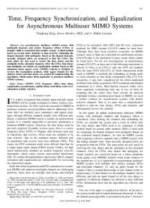
The Software Headend concept is derived from the Software Radio principle that was introduced in mobile communications. With respect to upstream transmission in CATV networks, major features of the Software Headend are: • Support of multiple standards on the same hardware platform. • Sampling of the complete upstream spectrum in the range of 5 - 65 MHz with one single wideband A/Dconverter. • Digital signal processing with programmable and flexible devices such as digital signal processors (DSPs) and field programmable gate arrays (FPGAs). Fig. 1 shows a top-level block diagram of the Software Headend for the reception and processing of upstream signals. The connection to the end-user devices via the cable network is illustrated in the left part, the connection to the wide-area network in the right part of Fig. 1. At the input of the Software Headend, the complete upstream spectrum is passed through a splitter. An amplifier adjusts the input signal to the dynamic range of the wideband A/D-converter that digitizes the signal with a resolution of 10 bit at the fixed sampling frequency f A = 153.6 MHz . After converting a selected channel with carrier frequency f C to baseband, the sampling rate is reduced to f B1 , a first intermediate frequency. This first downsampling block in Fig. 1 is a comprehensive element composed of a cascade of polyphase lowpass (LP) filters with decimation,

10. Dortmunder Fernsehseminar, 29. September - 1. Oktober 2003, ITG-Fachbericht 179, Seite 61-66

Splitter, automatic gain control and A/D converter Cable network Hybrid fiber coax (HFC)

s RX ( t )

LP-prefilter, 1st downsampling (cascaded in several stages) Pre-equalizer and matched filter inc. adaption of taps I

A D fA

Reference signal y B1,REF [ k ]

s TX ( t ) End-user devices (Cable modems, set-top-boxes, ...)

Fig. 1

Software Headend

NCO

y B1 [ k ]

C B1 ( z )

Q

fS

T-spaced equalizer inc. adaption of taps

CS(z)

f B1

Wide-area network (Internet, video server, PSTN, ...)

yS [ k ]

Reference signal y S,REF [ k ]

Signal detection f B2

Carrier and timing recovery + tracking

Symbol decision, demapping and error correction

MAC and higher layers

Top-level block diagram of the Software Headend

an optional sample rate conversion for DVB, and a matched filter with prototypes for all possible bandwidths specified in the DOCSIS and DVB standards. A pre-equalizer is placed in the area of this first intermediate frequency f B1 that depends on the symbol rate f S . Typically, f B1 is in the range of 1 - 20 MHz . The sampling rate is then further reduced in the signal detection unit so that carrier and timing recovery units operate at a low second intermediate frequency f B2 . The timing recovery unit triggers the second downsampling block in Fig. 1. Since the accuracy of the trigger signal is higher than the available data samples at f B1 , linear interpolation between two samples is performed. The output signal of that block contains the samples at symbol rate f S for further equalization, symbol decision, demapping and error correction. The carrier recovery unit triggers the numerically controlled oscillator (NCO) that adjusts carrier frequency and phase. All digital signal processing is realized in a simulation system with 16 bit fixed-point arithmetic. This simulation system of the Software Headend can be transferred to a hardware platform. Except for the first downsampling block that has to be implemented with an FPGA, the remaining elements can be realized with DSPs.

noise sources. In [4], important types of noise sources were investigated and grouped into the categories broadband noise, narrowband interferers and impulse noise with the sample functions n BB ( t ) , n NB ( t ) and n I ( t ) , respectively. Two transfer functions are depicted in Fig. 3. One is obtained from [5], a work in which an existing CATV network of a suburb near Stuttgart was measured and simulated. The other transfer function results from a test bed set up at the institut’s laboratory [4]. It should be mentioned that the frequency range up to 65 MHz for upstream transmission is not fully covered by the installed components in both cases. Concerning the overall simulation system, it is possible to select h ( t ) = h 1 ( t ) , h ( t ) = h 2 ( t ) or the ideal impulse response h ( t ) = δ ( t ) as well as up to three narrowband interferers at arbitrary center frequencies. Broadband noise and impulse noise are always present. s TX ( t )

Equalization

Basis for the design of an equalizer in the Software Headend is the model of a realistic upstream channel as well as the implementation of a module that generates a DOCSIS or DVB compliant transmit signal s TX ( t ) . When evaluating the performance of the Software Headend it is important that the simulation system of the transmitter is as ideal as possible. This was taken into account when designing the prototypes for the transmit-side impulse shaping filter and by using 32 bit floating-point arithmetic. Fig. 2 shows the channel model for upstream transmission. This model consists of the channel’s impulse response h ( t ) with the corresponding transfer function H ( 2πf ) and an additive noise term n ( t ) that is composed of typical

s RX ( t )

h(t )

Channel impulse response

Fig. 2

3

Resampling 2nd downsampling with linear interpolation

Noise sources n ( t ) = n BB ( t ) + n NB ( t ) + n I ( t )

Channel model for upstream transmission

4 2 0 -2 -4 -6 -8 -10 -12 -14 -16 -18 -20

Transfer function Lab H 2 ( f ) Transfer function Stgt H 1( f )

0

5

10

H( f )

[dB]

Fig. 3

15

20

25

30

35

40

45

50

55

60

65

f [MHz]

Transfer functions H 1 ( 2πf ) and H 2 ( 2πf )

Both equalizer blocks in Fig. 1 incorporate an algorithm to adapt the filter taps each upstream burst. The output signal y pos [ k ] of an equalizer is compared to a reference signal y pos, REF [ k ] where the index pos is a specifier for the frequency hierarchy. That reference signal is created from the preamble, a fixed and known pattern that precedes the data signal in every upstream burst. The preamble in the DOCSIS standard has variable-length and can be chosen arbitrarily. The length of the preamble is up to 1024 bits (up to 1536 bits for DOCSIS 2.0). Concerning the DVB standard, the DVB unique word has a length of 32 bit. To include equalization in the Software Headend, the following methods were considered: 1. Pre-equalization at the first intermediate frequency f B1 plus equalization at symbol rate f S as depicted in Fig. 1. 2. Equalization at symbol-rate without pre-equalization. 3. Enhanced pre-equalization without equalization at symbol rate. The pre-equalizer operates at the first intermediate frequency f B1 where complexity is still crucial. For that purpose, C B1 ( z ) is a non-recursive equalizer of degree N B1 . For equalization at symbol rate, non-recursive FIR and recursive IIR equalizers of degree N S were investigated. The filter taps are adjusted by the least mean square (LMS) or zero-forcing (ZF) algorithm. Tab. 1 shows typical values of N pos and compares the number of real-valued operations for the proposed methods. Lower and upper bounds are caused by minimum and maximum f B1 resp. f S .

this disadvantage. Although method 3 with N B1 = 10 at f B1 is not as good as N S = 8 at f S , the computational amount of this method is more than twice as high as that of method 1. Especially when migrating to a hardware platform, method 1 should be preferred. The quality of the equalization process can eventually be judged by the symbol error probability. All simulations yield lower error probabilities for the LMS algorithm than for the ZF algorithm. The following considerations that investigate the equalizer at symbol rate in more detail are based on the LMS algorithm therefore. The quadratic error is given by NS + MS

∑

J =

y S [ k ] – y S,REF [ k ]

2

(1)

k=0

where M S is the duration of the impulse response h ( t ) with respect to T = 1 ⁄ f S . Since y S [ k ] is a function of the equalizer taps b n , the minimum quadratic error J min = min J (2) bn

determines all b n , n = 0, …, N S . (2) leads to a linear equation system of 2 ( N S + 1 ) realvalued equations. The equalizer taps are obtained by inverting the 2 ( N S + 1 ) × 2 ( N S + 1 ) matrix of the equation system. This computation has to be performed while the preamble is transmitted. Afterwards, the taps are adjusted and the data signal is processed with the number of operations as given in Tab. 1. J min depends on N S . Tab. 2 lists several upstream transmission scenarios with transfer functions of Fig. 3, varying carrier frequencies, varying channel bandwidths and some narrowband interferers. The N S are computed in such a way that all scenarios lead to the same quadratic error J 0 .

Method

1)

2)

3)

Investigated structures

FIR, IIR

FIR, IIR

FIR

Investigated algorithms

LMS, ZF

LMS, ZF

LMS

N B1

2

0

10

Lab

22

NS

8

8

0

Stgt

Real-valued operations in 1 µs

36 - 800

8 - 196

86-1720

UpCarrier Narrowband stream frequency interferer(s) channel f C [MHz] f NB [MHz]

Channel bandwidth B [MHz]

NS

22.05

0.2

2

22

22.05

0.2

2

Lab

28

27.9, 28.2

0.8

3

Stgt

35

34.9, 35.3

0.8

3

Tab. 1 Comparison of equalization methods

Lab

22

22.05, 22.25

1.0

3

The pre-equalizer can be limited to N B1 = 2 when using method 1. This is sufficient to compensate phase shifts caused by signal delay and to adjust the amplitude. Introducing this simple pre-equalizer has major advantages for the data-aided synchronization units. This will be shown in the following section. Method 2 reduces the number of applicable synchronization techniques and results in poor estimates of the synchronization parameters. Less computational amount for equalization can not balance

Stgt

22

22.05, 22.25

1.0

3

Lab

22

22.05, 22.25

3.2

5

Stgt

22

22.05, 22.25

3.2

6

Lab

28

26.9, 28.2

3.2

6

Stgt

35

33.9, 35.4

3.2

8

Tab. 2 N S for several upstream transmission scenarios

Tab. 2 shows that N S is independent of the carrier frequency f C for channel bandwidths less than 3.2 MHz . If the bandwidth is 3.2 MHz , N S for h ( t ) = h 1 ( t ) is larger than for h ( t ) = h 2 ( t ) . This result is as expected since the attenuation of the transfer function H 1 ( 2πf ) varies in a wider range in the occupied frequency area.

4

Timing recovery

Data-aided timing recovery methods have significant advantages over general recovery methods [6]. The mathematical study [7] presents a new data-aided algorithm for DOCSIS with 16-QAM modulation and differential quadrant encoding. This study investigates signal detection, timing recovery and carrier recovery. The signal processing in [7] has been extended to support QPSK and 16-QAM each with optional differential encoding. Since all modulation schemes added in DOCSIS 2.0 (up to 128-QAM) have to use QPSK to transmit the preamble before switching to higher order modulation, all considerations hold for DOCSIS 2.0 as well. Furthermore, adaptions to the architecture as described in section 2 have been made. The following simulation results are based on the channel model and the equalization techniques as described in section 3.

4.1

sition of a peak indicates the beginning of an upstream burst and is used as a first coarse timing estimate. The simulations in Fig. 4 were configured in such a way that the peaks are located at different time instants just to make them easier to distinguish. The important aspect is the height of the peaks and the relation to the values A max that are computed when a random sequence is evaluated. The P = 16 DOCSIS peak is higher than the DVB peak because of the degree of freedom in the pattern of the symbol sequence. An improvement for DOCSIS can be achieved by increasing the length of the preamble. The peak nearly doubles by a factor of 2. 500

DVB Unique Word DOCSIS Preamble (P=16) DOCSIS Preamble (P=32)

✕

450 400

✧ ✛ ✕

✕✕

350 300

✛

250

✕ ✕

✛✛

200

✧ ✕ ✧✧ ✕ ✧ ✧ ✕ ✕ ✛ ✛ ✕ ✧ ✧ 100 ✕ ✕ ✛✕✕✕ ✛ ✕ ✛ ✛ ✧✛ ✕✛ ✧ ✕✛ ✛ ✕✕ ✛✛ ✛ ✛ ✛ ✛ ✛✛✛✕ ✕ ✕ ✧✕✕ ✛✛ ✕ ✛✛✛✕ ✕✕ ✕ ✕ ✛✛ ✛✧✧ ✕✕✛✕✛ ✕ ✛✕ ✕✕ ✛ ✕ ✛✕✕ ✛✛ ✕ ✕ ✧ ✛ ✕ ✛✛✕ ✛✧✛✛ ✕✧ ✛ ✕ ✛✕ ✛✛ ✛✛✛✧✛✕ ✕ ✛ ✕✛ ✛✕ ✕✧ ✛ ✧✕✕✧✕✕ ✕✛✕✕✕ ✛ ✕✛✛ ✛✕ ✧✕✧ ✧ ✕ ✛✕✧ ✛ ✧ ✛ ✛✕ 50 ✕ ✛✧ ✛ ✕ ✧ ✕ ✛✕ ✛ ✛✕✧✧✕ ✧ ✧ ✕ ✕ ✕ ✧✧✧✛✕✧ ✧ ✕ ✛ ✧ ✕ ✧ ✛ ✧ ✛ ✛✧ ✛ ✧ ✕ ✛ ✛ ✧ ✕✧ ✕ ✧✧✧✧ ✛✧✧ ✕✧✛✧ ✛✧ ✛✧ ✕✧✧ ✛✛ ✧ ✕✧ ✧ ✧✕ ✕✛ ✛✕ ✕ ✛✧✕ ✛✧ ✧ ✧✧✕✧ ✧ ✧✛ ✛✧✧ ✕✧✛✧✧✧✧ ✛ ✛ ✕ ✧ ✕ ✧ ✕ ✧ ✧ ✧ ✧ ✕ ✧ ✧ ✧ ✧ ✕ ✧ ✧ ✧ ✕✛ ✧ ✕ ✧ ✧✧ ✧ ✕ ✧ ✛ ✧ ✧✧✛ ✛ ✧ ✛✧ 0 ✧✧✧ ✛ ✛ ✛

150

0

10

20

30

40

A max

50

60

70

80

90

100

t ⁄ T B2

Signal detection: Evaluation of A max

Fig. 4

Signal detection

In a first step, the focus is on the signal detection block in Fig. 1. Within this block, the sampling rate is reduced from f B1 to f B2 . f B2 can be as low as 2 f S [8]. The signal at f B2 is denoted y B2 [ k ] . The detector tests y B2 [ k ] for a specific pattern that occurs when the preamble is received. Therefore the symbol sequence of the preamble is an important issue. For DOCSIS, the preamble is chosen in such a way that the transmitted symbol sequence is composed of P symbols alternating in the first and third quadrant of the complex plane. For DVB, the fixed pattern and the fixed length of the unique word can be used only. Signal detection is performed by evaluating (3) every symbol period.

4.2

As stated in section 4.1, the position of the peak value of A max gives the coarse timing position ˆt B2 with accuracy ˆt B2 ≤ T B2 ⁄ 2 (4) Since signal processing elements for detection and timing recovery operate at the low frequency f B2 , a higher precision reference signal of the preamble with sampling period T REF < T B2 is used for fine timing estimation. The optimum sampling instants ˆt 0 are computed by evaluating P ⋅ V B2

ε[k ] =

k

∑ yB2 [ k + lV B2 ]

l=1

(3)

V B2 is the number of samples per symbol period. To compare simulation results, it is best to chose the QPSK modulation format. The DVB unique word consists of P = 16 symbols in this case. Fig. 4 shows the values A max in a certain time interval for the DVB unique word and two DOCSIS preambles of length P = 16 and P = 32 . All results were obtained with equalization method 1. When the preamble passes through the detector, a peak with linear increase and decrease can be observed. The po-

∑

l=0

T B2 T B2 y B2 [ l ] – y B2,REF l ------------ + k – -------------T REF 2T REF min ε [ k ] → k 0

P

A max = max

Fine timing

k

2

(5) (6)

and ˆt 0 = ˆt B2 – T B2 ⁄ 2 + k 0 T REF The accuracy of ˆt 0 improves to ˆt 0 ≤ T REF ⁄ 2

(7) (8)

Simulation results for timing acquisition are shown in Fig. 5. As an example, several cases for the normalized timing error ( ˆt 0 – t 0, id ) ⁄ T , where t 0, id is the ideal sampling instant are plotted for varying signal-to-noise ratio (SNR). 3 simulations in Fig. 5 are based on equalization method 1.

0.5 0.4

■

0.3 0.2

DOCSIS, 16-QAM, Equalization method 1 DOCSIS, QPSK, Equalization method 1 DVB, QPSK, Equalization method 1 DOCSIS, 16-QAM, Equalization method 2

■ ✛

✕ ✛

✛ ✧ ✧

✧ ✛ ■ ✕

✛

■ ■ ✕ ■ ✛ ✧ ✛ ✛ ✛ ✧ ■ ✕ ■ ✕ ■ ■ ✧ ✕ ✛ ✧ ✕ ✧ ✧ 0 ✕ ✕ ✕ ✕ ✕ ■ ✧ ■ ✧ ■ ✧ ■ ✧ ■ ✧ ■ ✧ ■ ✧ ■ ✧ ■ ■ ■ ■ ✧ ✛ ✧ ✛ ✧ ✛ ✧ ✛ ✛ ✛ ✧ ✛ ✛ ✛ ✛ ✛ ✛ ✛ ✧ ✛ ✧ ✛ ✧ ✛ ✕ ■ ■ ✧ ■ ■ ■ ✕ ✕ ■ ■ ✧ ■ ✕ ✕ ✧ ✛ ✧ ✛ ✛ ✕ ✕ ✕ ✕ ✕ -0.1 ✕ ✕ ✛ ✛ ✕ ■ ✕ ✕ ✕ ✕ -0.2 ✕ ✕ ■

0.1

✧ ✧ ✕

✛ ✧

-0.3

ˆ – ∆f Fig. 6 shows the carrier frequency offset error ∆f normalized to the reference frequency f R = 1 kHz as a function of the signal-to-noise ratio. The parameters for these simulations are a DOCSIS based system, 16-QAM modulation, equalization method 1 and channel bandwidth B = 0.8 MHz . Two curves with preamble length P = 16 have carrier frequency offsets ∆f equivalent to 0 ppm and +50 ppm . Two further curves have preamble length P = 32 . We can see that doubling the preamble length results in approximately half of the carrier frequency offset error.

-0.4 0.5

-0.5 0

2

4

6

8

10 12 14 16 18 20 22 24 26 28 30

( ˆt 0 – t 0, id ) ⁄ T

Fig. 5

SNR [dB]

✛ ✧ ✛ 0.4 ✧ ✛ ✧ ■ ✕ 0.3 ✕ ✕ ■

Estimation error of the optimal sampling instants

0.2

The normalized timing error for these simulations is below 0.05 for a signal to noise ratio greater than 10 dB . A further simulation with equalization method 2 permanently falls below 0.05 not until 21 dB . The acquisition parameter ˆt 0 is adjusted every upstream burst. Additionally, maximum likelihood and mean square error tracking loops [6] were implemented after the acquisition process to further improve and stabilize estimation results. The timing information for the optimum sampling instants is passed to the resampling unit in Fig. 1. This unit performs downsampling to symbol rate. Since the data signal at f B1 may not contain the high-precision sampling instants, linear interpolation between two samples is applied.

✛ ✧ ✛ ✧

✛ ✧

✕

■ ■

P=16, 0ppm P=16, 50ppm P=32, 0ppm P=32, 50ppm ✛ ✧

■ ✕ ✕ ■

0.1

✛ ✛ ✧

✕ ■

✧

✛ ✛ ✧ ✧

✛ ✧ ✕ ■ ✕ ✕ ✕ ■ ✕ ■ ■ ■

0 0

2

4

6

8

10

✛ ✛ ✧ ✧

✛ ✛ ✧ ✧ ✧ ✛ ✧ ✛ ✕ ✛ ✛ ■ ✕ ■ ✕ ✕ ✧ ■ ✕ ■ ✕ ✧ ■ ■ ✕ ✛ ✧ ■ ✧ ✛ ✧ ✛ ✛ ✛ ✕ ■ ✕ ■ ✕ ✧ ✕ ✧ ■ ■ ✛ ✛ ✕ ■ ✧ ✕ ✕ ✧ ✕ ✧ ✕ ✕ ✧ ✕ ✧ ✕ ■ ■ ■ ■ ■ ■ ■ ✛ ✧ ✛ ✛ ✛

12

ˆ – ∆f ) ⁄ f ( ∆f R

Fig. 6

14

16

18

20

22

Carrier recovery

5.1

Fig. 7

ˆ = ∆f

∑

k=1

(9)

w [ k ] is the smoothing function [7]: 3P – P ⁄ 2 + 1 2  k---------------------------w [ k ] = ---------------------1 – 2   P⁄2 2( P – 1)

(10)

✧

✧

0.3

arg y B2 [ k ] w [ k ] ⋅ ------------------------2πV B2

P=32, 0dB P=32, 8dB P=32, 16dB

✧

Among several techniques for carrier recovery, the extension of [7] provides very good results at low intermediate frequencies f B2 . Similar to timing recovery, this data-aided technique uses the preamble in form of a reference signal to estimate the two acquisition parameters carrier ˆ and carrier phase θˆ 0 . Tracking is refrequency offset ∆f alized with a feedback-loop to the numerical controlled oscillator (NCO).

P–1

28

30

In Fig. 7, the normalized carrier frequency offset error is plotted as a function of ∆f (in ppm). Both standards specify a maximum carrier frequency deviation of 50 ppm . The simulations are carried out at 3 different signal-tonoise ratios and for P = 32 . Fig. 7 clearly shows that the proposed algorithm is not sensitive to ∆f .

✧

The carrier frequency offset ∆f can be estimated from the signal y B2 [ k ] . It holds:

26

Carrier frequency offset estimation vs. SNR

0.4

Carrier frequency offset estimation

24

SNR [dB]

0.5

5

✧ ✛ ■ ✕

✧

✧

✧

✧

✧ ✧

✧

✧

✛ ■

✛

✛

■

■

✧

✧

✧

✧

✧ ✧

✧

✧

✧ ✛ ■ ✧

0.2 ✛

0.1 ■

✛

✛

✛

■

■

■

0 -50

-40

ˆ – ∆f ) ⁄ f ( ∆f R

5.2

✛ ■

-30

✛

✛

✛

■

■

■

-20

✛ ■

-10

✛ ■

0

10

✛ ■

✛ ■

20

✛ ■

✛ ■

30

✛ ■

✛ ■

40

✛

✛

■

■

50

∆f [ppm]

Carrier frequency offset estimation vs. ∆f

Carrier phase estimation

The approach [7] first compensates the carrier frequency offset and then uses the reference signal y REF [ k ] of the preamble to estimate the carrier phase θˆ 0 . In a longer derivation, the conditional probability density function (pdf) of the observed preamble symbol sequence for a given θ 0

is determined first. Then, the likelihood function of this pdf is computed. Finally, the likelihood function is maximized with respect to θ 0 . The result is: P–1

θˆ 0 = arg

∑

y REF [ k ] ⋅ a k ∗

(11)

k=0

where a k ∗ is the conjugate complex preamble sequence. The carrier phase estimator (11) does not change when the approach is generalized in order to support the architecture of the Software Headend. Simulation results for carrier phase estimation are depicted in Fig. 8 and Fig. 9. The carrier phase error θˆ 0 – θ 0 normalized to the reference phase θ R = π ⁄ 10 is plotted as a function of the signal-to-noise ratio and the carrier phase θ 0 , respectively. The set of parameters is the same as in the previous subsection. The improvement when doubling the preamble length is approximately the factor 2 again (see Fig. 8). The carrier phase estimation is also not sensitive to any carrier phase randomly distributed in [ – π, π ] as it can be observed in Fig. 9. 0.5

P16, 0 P=16, Pi P=32, 0 P=32, Pi

0.4

✧ ✛ ■ ✕

✛ ✧ ✛ ✧ ✧ ✛ ✛ ✧ ■ ✛ ✛ ✧ ✕ ✧ ■ ✛ ✕ ✛ ✧ ■ ✧ 0.1 ✛ ■ ✕ ✧ ✕ ✛ ■ ✕ ✧ ■ ■ ✕ ✛ ✛ ✧ ✕ ■ ✕ ✛ ✧ ✧ ■ ✕ ■ ✕ ■ ✧ ✛ ✛ ✧ ✛ ✕ ■ ✕ ■ ✛ ✕ ■ ✧ ✕ ✛ ✧ ■ ✧ ✛ ✧ ✕ ■ ✕ ✛ ✧ ■ ✛ ✕ ✕ ■ ✧ ✕ ■ ■ ✕ ■ ✧ ✛ ✕ ✛ ✧ ■ ✧ ✕ ✕ ✛ ✧ 0 ✕ ■ ■ ■ ■ ■ ■ ■ ■ ■ ✛ ✧ ✛ ✧ ✛ ✧ ✛ ✧ ✛ ✧ ✛ ✛ ✕ ✕ ✕ ✕ ✕ ✧ ✕

0.2 ✕

2

4

6

8

10

12

( θˆ 0 – θ 0 ) ⁄ θ R

Fig. 8

14

16

18

20

22

24

26

28

P=32, 0dB P=32, 8dB P=32, 16dB

✧ ✛ ■

30

SNR [dB]

Carrier phase estimation vs. SNR

0.5 0.4 0.3 0.2 ✧

✧

✧

✧

✧

✧

✧

✧

✧

✧

✛ ■

✛ ■

✛ ■

✛ ■

✛ ■

✛ ■

✛ ■

✛ ■

✛ ■

✛ ■

-0.8

-0.6

-0.4

-0.2

0

0.2

0.4

0.6

0.8

1

✧

0.1 ✛

0■ -1

( θˆ 0 – θ 0 ) ⁄ θ R

Fig. 9

θ 0 [Pi]

Carrier phase estimation vs. θ 0

Conclusions

We have investigated equalization and synchronization aspects in the architecture of a Software Headend. The Software Headend can be used for flexible digital signal processing of upstream signals in CATV networks. The frequency hierarchy of a Software Headend with optimized levels for minimum signal processing power requirements was outlined. Equalization in the Software Headend is should be implemented by a 2-tap pre-equalizer at a first intermediate frequency and an 8-tap equalizer at symbol rate. This cascade of 2 equalizers can handle realistic upstream transmission scenarios the best way. The implemented data-aided synchronization elements operate well even at low SNR. The performance for DOCSIS can be enhanced when the length of the preamble is increased. The fine timing estimation and the carrier frequency offset estimation are very accurate up to 10 dB, the carrier phase even up to 6 dB. Carrier frequency offset and carrier phase can vary in the specified range without reduction of the overall performance.

7

0.3

0

6

References

[1] DOCSIS 2.0 Radio Frequency Interface Specification, SP-RFIv2.0-I03, Dec. 2002. [2] ETSI standard ES 200 800 v1.3.1, "DVB interaction channel for Cable TV distribution systems," Oct. 2001. [3] A. Braun, J. Speidel, H. Krimmel, "The Software Headend Architecture - A New Approach for MultiStandard CATV Headends," IEEE Conference on Consumer Electronics (ICCE), Los Angeles, Digest of Technical Papers, pp. 156-157, Jun. 2002. [4] Pfletschinger, Stephan, "Multicarrier Modulation for Broadband Return Channels in Cable TV Networks," Dissertation, Universität Stuttgart, Shaker Verlag, 2003. [5] Brendle, Peter, "Breitbandiger Rückkanal im Kabelfernsehnetz für Multimedia-Anwendungen", Dissertation, Universität Stuttgart, Shaker Verlag, 1998. [6] U. Mengali, A. N. D’Andrea, "Synchronization Techniques for Digital Receivers," Plenum Press, Nov. 1997. [7] J. Wang, J. Speidel, "Packet Acquisition in Upstream Transmission of the DOCSIS Standard," IEEE Trans. on Broadcasting, vol. 49, no. 1, pp. 26-31, Mar. 2003. [8] J. Wieland, "Erweiterung und Optimierung der Taktrückgewinnung für Rückkanalsignale in Kabelfernsehnetzen," Studienarbeit, Institut für Nachrichtenübertragung, Universität Stuttgart, 2003.