Equilibrium traffic assignment on large Virtual Networks: Implementation issues and limits for multi-modal freight transport
Bart Jourquin*,** and Sabine Limbourg* * Facultés Universitaires Catholiques de Mons (FUCaM), Group Transport & Mobility (GTM) Mons Belgium e-mail:
[email protected] ** Universiteit Hasselt Diepenbeek Belgium EJTIR, 6, no. 3 (2006), pp. 205-228
Received: February 2005 Accepted: March 2006
Multi-Modal freight models are traditionally built following the well known “four steps model” in which generation, distribution, modal-split and assignment are seen as separated modules. An alternative approach, now implemented in some software, is to represent the multi-modal network by means of a “mono-modal” one, in which each particular transport operation (loading or unloading operation, transhipments ...) is represented by a dedicated “virtual link”, that represents a specific operation in the transportation chain. This approach, promoted by several authors, often referenced to as “super networks” or “virtual networks”, is proven to give interesting results, but has the drawback to generate much larger networks than the pure geographic representation of the studied area. It has also some kind of “hidden trap”, linked to transport distances, that will be presented in this paper and that can only be solved using appropriate assignment techniques. This paper presents some results obtained on a large multi-modal network, using different equilibrium assignment algorithms, in order to test their ability to give an appropriate solution to the “distance trap”. It however concludes that the implementation of classical equilibrium assignment techniques leads to solutions that are barely different from the one obtained by a simple all-or-nothing assignment, opening the way to alternative multi-flow solutions.
206
Equilibrium traffic assignment on large Virtual Networks: Implementation issues and limits for multi-modal freight transport
Keywords: freight transport, multimodal, assignment, GIS.
1. Introduction Until a few years ago, transport models were essentially focused on passengers’ flows. More recently, some freight specific network models have been developed but, like passengers models, they are essentially analysing networks from a "link" point of view rather than from a "node" point of view. Even if some of them deal to some extent with the different operations performed at the nodes, i.e. loading /unloading, transhipment or simple transit, their output still targets mainly transport flows on the networks. As a result of a trend towards economic globalisation, just in time deliveries and road transports expansion, a great deal of attention is paid nowadays to reorganising the networks and intermodal transports, developing new technical bundling concepts in order to substitute transport solutions with less negative external effects to direct road transport. Thus, there is a need for a better modelling of the functions assumed by nodes, i.e. terminals and transhipment platforms, because the costs of the operations performed at these nodes are important in the total cost of transport. Indeed, a geographical multimodal transport network is not only made of links like roads, railways or waterways, on which vehicles move but also of connecting infrastructures like terminals or logistics platforms that exist at the nodes. To analyse transport operations over the network, costs or weights must be attached to the links over which goods are transported as well as to the connecting points where goods are handled. However, most of these transport or handling infrastructures can be used in different ways and with different costs. For example, boats of different sizes and operating costs can use the same waterway; at a terminal a truck's load can be transhipped on a train, bundled with some others on a boat or simply unloaded as it reaches its destination. Normally, the costs of these alternative operations are different. In order to model this, one of the solutions is to represent each kind of operation in a node as a specific link of a “virtual network”, for which a relevant cost is then computed. Beyond this brief introduction, this paper will present an overview of the “virtual network” methodology implemented in specific software and its “hidden trap”. It will then discuss the most used assignment techniques and how they can be applied to virtual networks. Finally, the performances of these methods will be discussed on a test and a large real-world network.
2. Virtual networks and software implementation 2.1 The building of a virtual network: an intuitive approach A simple geographic network does not provide an adequate basis for detailed analyses of transport operations as the same infrastructure, link or node, can be used in different ways. To solve this problem, the basic idea, initially proposed by Harker (1987) and Crainic et al. (1990), is to create a virtual link with specific costs for a particular use of an infrastructure. The concept of “supernetworks” proposed by Sheffi (1985), that proposed “transfer” links between modal networks also provides a somewhat similar framework. The NODUS software proposes a methodology and an algorithm that creates in a systematic and automatic
European Journal of Transport and Infrastructure Research
Jourquin and Limbourg
207
way a complete virtual network with all the virtual links corresponding to the different operations, which are feasible on every real link or node of a geographic network. This systematic and automatic approach, built upon a special codification of the virtual node labels, is probably the biggest benefit over other software tools such as STAN (Crainic et al. (1990)), in which most of the tasks that are possible at a given node are to be introduced “by hand”. The software, which is completely geographically referenced in its latest version, and its underlying methodology were already discussed in Jourquin (1995) and Jourquin and Beuthe (1996). More recent works (see for instance Tavasszy (1996)) include some discussion about virtual networks and the software that implements them. The methodology can be presented first in an intuitive way by using the example of a simple multi-modal network, as shown in figure 1. This network consists of 4 nodes (a, b, c, d) and 5 links (1 to 5). The “W” links represent waterways and the “R” links rail tracks. The numbers after these letters correspond to the transportation means that can be used on the links. So, “W1” represents a waterway that can only support small barges and “W2” a waterway that can be used by both small and large barges. a
1 (W2)
b
3 (R1)
5 (W1)
2 (W1)
c
4 (R1)
d Figure 1. Multimodal network To go from node “a” to “d”, it could be that route through links 1+3 and using large barges and trains is less expensive than route 5, using exclusively small barges. Indeed, computing costs and routes on this kind of networks is not immediate: a) Different costs can be assigned on a single link, depending on which transportation means is used. In this example, the use of a small barge on link 1 has a different cost than the use of a large barge on the same link; b) The same is true for the nodes: in the given example, the simple transit of a small barge from link 1 to link 2 can be done at no cost, but the transhipment from a large barge onto a train that will go on link 3 represents an important cost. This problem can be usefully handled on the corresponding virtual network illustrated in Figure 2, provided that the relevant costs are attached to each of the virtual links. As can be seen, the solution involves the creation of a set of virtual nodes and a set of virtual links connecting these nodes. Each real link has been split in as many virtual links as there are possible uses; their end-nodes are connected by new virtual links corresponding to simple transit or transhipment operations at the real nodes.
European Journal of Transport and Infrastructure Research
208
Equilibrium traffic assignment on large Virtual Networks: Implementation issues and limits for multi-modal freight transport
In this way, this network with multiple means use is represented by a unique but more complex network on which each link corresponds to a unique operation with a specific cost. Then, one cheapest path can be computed by means of an algorithm such as the one proposed by Dijkstra (1959). The resulting solution is an exact solution, taking all the possible choices into account. It is now possible to demonstrate how virtual networks are built on the basis of a rather simple, though somewhat complex notation, which provides a convenient way to link cost functions to virtual links. Table1 enumerates the elements of the real network. a1W1
b1W1
b2W1
a5W1
c2W1
c4R1 a1W2
b1W2 b3R1
d5W1
d4R1
Figure 2. Partial virtual network Table 1. Real network Link 1 2 3 4 5
Origin node a b b d a
Destination node b c d c d
Type of link W2 W1 R1 R1 W1
In a first step, the virtual links corresponding to the real links, i.e. rail tracks, etc., must be generated. These are defined in table 2 by their end-nodes, the notation of which indicates successively the real node, the real link, the mode and the means they refer to. Table 2. Travelling links Real links End-nodes of virtual links 1 a1W1 b1W1 a1W2 b1W2 2 b2W1 c2W1 3 b3R1 d3R1 4 d4R1 c4R1 5 a5W1 d5W1
European Journal of Transport and Infrastructure Research
Jourquin and Limbourg
209
In a second step, these virtual links must be connected by transit or transhipment virtual links. To keep things as simple as possible, we just enumerate in table 3 the virtual links related to node “b”. They can be viewed in figure 2. In this network, the boldfaced links represent the links of the real network, possibly split up in several virtual links the dotted links represent the simple transit virtual links, while the transhipment links are indicated by a thin continuous line. Table 3. Connecting virtual links to node b Real node End-nodes of virtual links B b1W1 b2W1 b1W2 b2W1 b1W1 b3R1 b1W2 b3R1 b2W1 b3R1
In general, the weight given on a link can very well vary with the direction it is used: loading and unloading operations for instance don’t have necessarily the same cost, and the cost of going upstream on a river is normally higher than going downstream. To solve this problem related to the asymmetry of cost functions, all the virtual nodes are doubled at generation time by adding a + or a – sign to their code; by the same token, all links are split into two oriented arrows connecting these new nodes, as illustrated in figure 3. Those “doubled” virtual nodes and oriented links also permits to avoid “unwanted movements”, like an unloading followed by a loading operation to circumvent a forbidden transhipment operation. -
b1W1
b1W2
b000
+
+
-
-
+
b2W1
+ +
-
b3R1
Figure 3. Detailed virtual network at node
European Journal of Transport and Infrastructure Research
210
Equilibrium traffic assignment on large Virtual Networks: Implementation issues and limits for multi-modal freight transport
Such a network can be completed by introducing entry and exit nodes to the network. This can be done by the creation of additional virtual nodes associated to loading and unloading operations at nodes where these operations are possible. Those entry or exit points in the virtual network are referenced by adding “000” to the real node number. They must also be connected to other nodes by appropriate virtual links. These additional virtual nodes and links appear in the upper part of figure 3. In order to implement the above code convention, the virtual nodes are coded in the following way: a plus or minus sign, 5 digits for the real node number, 5 digits for the real link number, 2 digits for the transport mode and 2 digits for the transport means. Each label is thus represented by a signed 14 digits number. A virtual link can thus be simply characterized by its origin and destination virtual nodes. After this overview of the basic methodology, it is necessary to explain the characteristics of the cost functions and how they are connected to the virtual network. As usual in transportation analysis (see, for example, Kresge and Roberts (1971), or Wilson and Bennet (1985)), the "generalised cost" concept is used, which allows to integrate all factors relevant for transport decision making in terms of monetary units. The concept can be defined in different ways according to whether it is the point of view of the shipper or the carrier which is taken, and according to the used unit of reference, i.e. tons, tons-km, vehicles, etc. The specific cost functions which compose the generalised cost, obviously, must be coherent across modes and means, but their functional forms can be freely chosen. The four types of virtual links require specific cost functions, containing the following elements: a) All the costs related to moving a vehicle, such as labour, fuel, insurance, maintenance costs, or tariffs; b) The inventory costs of the goods during transportation and other time related costs; c) Handling and storage costs or tariffs, including packaging, loading and unloading and services directly linked to transport. d) All residual indirect costs like general administrative services which may be assigned to transport on an average basis. 2.2 Computing shortest paths on networks The contemporary transport systems are used in an intensive way and are often congested in various degrees, particularly in urban areas. Transport models have to determine how the traffic is distributed over the transport network of which the structure and the capacity are known. This is the assignment problem. The results of the assignment, which depend on the sophistication of the implemented method, include an estimate of flows, travel duration and/or corresponding costs, for each link of the network. Unless no capacity constraints are taken into account (All-Or-Nothing assignment), an assignment consists in the distribution of the traffic on a network considering the demand for trips as well as the capacity of the network; the assignment methods distribute the traffic over a network in order to obtain an equilibrium solution. This type of problems can be solved by means of optimisation methods. Other assignment techniques try to spread the flow over several alternatives routes, trying to take into account behavioural considerations. This paper deals with the methods intended to model flows of commodities on large interurban, regional and international multimodal freight networks, like those generated by the virtual network methodology.
European Journal of Transport and Infrastructure Research
Jourquin and Limbourg
211
With the exception of the new “origin-based assignment”, developed by Bar-Gera and Boyce (2003), which for a given origin considers all the destinations together and optimises the routes serving them1, all the equilibrium assignment methods are based on the “All-orNothing” (AoN) algorithm. The principle of this algorithm is to compute the minimum weight path between each pair of origin and destination, and to allocate the total demand to be transported between these nodes onto this single path. The AoN assignment is itself based on shortest path computations. The efficiency of this latest algorithm is crucial and it is important to choose the one that gives the fastest results for a given problem. The algorithm of Dijkstra solves the problem of the shortest path from an origin to all the possible destinations. The one developed by Johnson finds all the shortest paths between all the pairs of nodes of the graph, combining the algorithm of Bellman-Ford and Dijkstra. The implementation of the algorithm in the computer software, using efficient data structures, also has an important effect on the performances. For solving the shortest path problem Zhan and Noon (1998) have tested 15 algorithms, among which Bellman-Ford-Moore, Dijkstra, Pape, or Pallottino on real road networks; they conclude that the implementation of Pape is probably the most efficient but that it is worthwhile to consider Dijkstra’s implementations in case a subset only of the destinations from a given node is to be computed. That is exactly the case we have to cope with, as our origindestination (O-D) matrixes do not contain a demand for each possible O-D pair. The efficiency of an algorithm can be measured using the notion of time complexity2, which can be defined as the number of steps needed to solve an instance of a problem, expressed as a function of its size of. If a shortest path algorithm solves, in the worst case, a problem with N nodes in a time c.N², where c is independent of the input size, the required computational effort is O(N²). This is the case of Dijkstra’s algorithm whereas Johnson’s is O(N³). These complexities are obtained if the input data is stored in linear arrays. These algorithms can be improved (faster search and insert operations) by using binary heaps instead of linear arrays. Using these heaps, the complexities become respectively O(Mlog2N) and O(NMlog2N). Fibonacci heaps are even more efficient than binary heaps, decreasing the time complexity of the shortest paths algorithms. The detailed virtual network generated from the European network that we used has more than 500.000 virtual links (M) and 140.000 virtual nodes (N), of which about 1500 (X) are potential (un)loading nodes. As explained earlier, this latest characteristic indicates that Dijkstra’s algorithm is probably the most suitable, since paths must be computed from only a small number of potential origins. As shown in table 4, the algorithm of Dijkstra, with a heap implementation, seems to be the most efficient when applied on a virtual network (which is a low-density graph, since the number of links is much smaller than the square of the number of nodes). However, despite the fact that, from a theoretical perspective, the Fibonacci heap implementation should perform better than a binary heap based implementation, it appears that the later performs better on the problems that are dealt with here. Indeed, the Fibonacci heap implementation gives smaller execution times only in the most unfavourable cases. During the numerous tests we have performed, these cases represent only about 15% of the test sets. On __________ 1
Unfortunately, this method is not yet enough documented to be easily implemented in our software A complete presentation of the time complexity computation of the algorithms can for instance be found in Cormen et al. (2001), chapter 24.
2
European Journal of Transport and Infrastructure Research
212
Equilibrium traffic assignment on large Virtual Networks: Implementation issues and limits for multi-modal freight transport
average, we found out that the computing time for a complete O-D matrix using a Fibonacci heap is about 50% slower than with a binary heap. This is due to the fact that the computer cost of dealing with the Fibonacci heap appears often to be higher than the search cost in simpler heaps. Table 4. Complexity of shortest-path algorithms Data structure Linear (worst case)
Binary heap (worst case)
Fibonacci heap (amortised analysis1)
Dijkstra’s algorithm Executed X times
O(XN²)
O(XM log2N)
O(XN log2N+XM)
Johnson’s algorithm
O(N³)
O(NM log2N)
O(N² log2N+NM)
Given: N number of nodes M number of links X number of nodes that are a potential origin or destination 1 An amortised analysis differs from an average case analysis because it guarantees an average performance for the worst cases.
Finally, in order to obtain still faster results, we have introduced a stop criterion in Dijkstra’s algorithm. Indeed, it stops as soon as the paths to all the relevant destinations are computed instead of doing the work for all possible destinations. This improves the computing time by more than 50% on real cases, because the commodities are sent to only a few destinations in most cases. Moreover, these destinations are often relatively close to this origin. 2.3 A promising methodology with a hidden trap The used cost functions for the different transport operations can be relatively detailed and complex, and for instance take into account the nature of the transported goods. This can lead to the use of different transportation modes for different commodities. Nevertheless, the aggregation level of the origin-destinations matrixes that can be produced for very large areas is such that one cannot guess that, for a given category of commodities, everything is transported by the same transportation mode. Indeed, the demand at the European level for instance is often only available at the NUTS1 or NUTS2 level. Even when more sophisticated techniques are used to obtain city to city relations, it is a nonsense to consider that everything that is sent from a given city to another uses the same, unique, transport mode: a factory located nearby a railway station will most probably more often use railway transport than another, located in the same city, but far from the station. Finally, even for a given point-topoint relation between two factories, some internal logistic considerations make it sometimes useful to use alternative transportation modes. In the classical models, the modal choice is applied as a separate step. In other words, in such an approach, all the quantities for a given mode are separately assigned on their respective modal networks in order that each mode is used on short and long distances with no particular limitations. However, on “virtual networks”, an assignment doesn’t search for a cheapest physical itinerary, but for a cheapest path that includes all the (un)loading, transit and transhipment operations, so that the simple notion of transportation mode loses a lot of its original meaning, cre-
European Journal of Transport and Infrastructure Research
Jourquin and Limbourg
213
ating a new problem. This will now be illustrated by means of a simple example. In table 5, a small demand matrix is described, that contains data for two transportation modes. The last column is obviously not an input data but a simple computation based on the two previous columns. From this table, it is easy to conclude that 17 tons are transported by mode 1 and 16 by mode 2. The tons.km for the two modes are respectively equal to 3850 and 5400. Table 5. Input data for simple example Mode 1 1 2 2 1 2
Distance 100 150 200 300 400 500
Tons 4 7 6 4 6 6
Tons.km 400 1050 1200 1200 2400 3000
This example clearly illustrates that distance cannot be considered as the only explanatory variable and that there exists some unobserved factors that explain the mode (and route) choice for individual shipments. This is a classical point that has often legitimated the use of random utility models to describe actual flows on a network. In passenger transport models, the use of such a stochastic approach is useful because the behaviour of the human being during his journeys can be influenced by a lot of, sometimes subjective, factors. This is particularly true in urban networks. This is less the case for long haul freight transport. However, in large scale models, the details of the network is not sufficient to identify the exact location of each firm and the modal networks it is connected to. Finally, the nature of the demand matrixes is so that, even in the best cases, information is only available from city to city and not from a particular firm to another. All these factors make the demand table 1, in which the different transport modes are used on different distance classes, an often encountered and plausible scenario. Consider that the two transportation modes have linear cost functions, so that cost = A + B*distance. The values for A are 2 for mode 1 and 55 for mode 2. The values for B are set to 0.5 and 0.3 respectively. Figure 4 illustrates these two cost functions, and it can clearly be seen that mode 1 will be chosen for the three first elements of the demand matrix, because they are related to distances that are shorter then the break-even distance. Mode 2 will be used for the remaining entries of the matrix. Thus, 17 tons will be assigned to mode 1 and 16 to mode 2, which are the expected figures. But only 2650 tons.km will be transported by mode 1 and 6600 by mode 2.
European Journal of Transport and Infrastructure Research
214
Equilibrium traffic assignment on large Virtual Networks: Implementation issues and limits for multi-modal freight transport 275 250 225 200 175
Cost
150 125
Mode 1 Mode 2
100 75 50 25 0 100
200
300
400
500
Distance
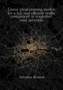
Figure 4. Original cost functions The cost functions can obviously be recalibrated in order to try to obtain a better fit in terms of tons.km. For instance, figure 5 illustrates the cost functions when the values of A and B are respectively fixed to 52 and 0.35 for mode 2, the values for mode 1 remaining unchanged. In this case, the four first lines of the demand matrix will be assigned to mode 1, for a total of 3850 tons.km, which is perfectly right. But now, 21 tons will be transported by mode 1, which is too much. This simple example shows that, using a simple All-Or-Nothing assignment, it is impossible to calibrate an assignment on both the transported quantities (tons) and the flows (tons.km) when virtual networks are used to avoid separate modal-choice and assignment models. The only way to solve this “distance trap” is to implement techniques that don’t, for a given distance (and origin-destination pair), assign all the demand on the same path (and thus maybe same mode) on a virtual network. The first techniques one might thing to are the equilibrium assignment algorithms, which spread the flow over several alternative routes, according to the flow on the used links. Their implementation will now be discussed. This is the main topic of this paper.
European Journal of Transport and Infrastructure Research
Jourquin and Limbourg
215
275 250 225 200 175
Cost
150 125
Mode 1 Mode 2
100 75 50 25 0 100
200
300
400
500
Distance
Figure 5. Modified cost functions
2.4 Cost functions and congested links As just discussed, a simple implementation of the AoN algorithm presents some limits because it is often observed that the flow of transport between two given nodes is distributed over various alternative routes. Two main reasons can explain this phenomenon: the capacity constraints of the network and the fact that all the users don’t have the same perception of the costs of the different alternative routes. Both reasons induce a spreading of the flow over several routes. But do the equilibrium assignment techniques give an appropriate answer to the “distance trap “ problem? The equilibrium algorithms take into account the variation of the transportation costs according to the assigned flow, considering that the distribution of the traffic over the network is the result of an interaction between the supply and the demand for transport. They try to implement the second equilibrium condition of Wardrop (1952), who stated that: Under equilibrium conditions traffic should be arranged in congested networks in such a way that the average (or the total) travel cost is minimised. It is important to note that the implementation of these methods on a virtual network makes it possible to observe transfers of flow not only between different routes, but also between various transportation modes. Indeed, in opposition to the classical four stages models (generation, distribution, modal-split and assignment), virtual networks, which explicitly decompose all the tasks in the transportation chain, combine modal split and assignment in a single step. Thus, an alternative route could very well be used, totally or partially, by another mode and/or means of transport than the ones that were used on the initial route, without any explicit modal-split. This is probably the most important contribution of the use of equilibrium assignment methods on virtual networks and this will be illustrated in the next section.
European Journal of Transport and Infrastructure Research
216
Equilibrium traffic assignment on large Virtual Networks: Implementation issues and limits for multi-modal freight transport
The discrete choice models often used in the classical four stages approach include an error term describing non-explained variation, as well as random coefficients explaining variations of preferences. The supporters of these methods often argue that these methods avoid that two competing routes with almost the same costs would be assigned all-or-nothing if there are no capacity problems. This problem is at least partially addressed in our model, because the demand is split into 10 categories of commodities, each of them having its own set of cost functions. Moreover, the speed-flow curve is not flat as long as the capacity of a link is not reached, making it possible that the flow is spread over several routes, even if saturation is never observed on any link. Finally, the introduction of random coefficients in order to take into account behavioural aspects (probability to choose a given route) is much more linked to stochastic (equilibrium) traffic assignment models, which are not discussed in this paper. The equilibrium assignment models require cost functions which are related to the flow on the network. Such a relation can be generally expressed as: Ca=Ca({V}). In principle, the cost on link “a” should be a function of the flow V on the total network and not only on the link itself, because the flow on a given link is also influenced by the neighbourhood. This is usually simplified by considering that Ca=Ca(Va), i.e. that the cost on link “a” is a function of the flow Va on it. A good cost function must be realistic, nondecreasing, monotonous, continuous and differentiable and should not generate infinite costs if the flow is equal or higher than the capacity in order to always ensure a solution. Many functions were proposed to describe this relation. Ortúzar and Willumsen (1990) give a good overview of them. The most used are: V /K
a) Smock (1962) : C = C 0 e where C is the cost for a given flow V, C0 is the cost at free flow and K the capacity of the link. b) Overgaard (1967) generalises the previous function: C =C α β (V / K) 0
c) The Bureau of Public Roads (BPR, 1964), USA, proposes the standard function which β is most often: C = C0 1 + α (V / K ) We used latest function with α= 0.15 and β= 4. These values may deem to be doubtful because they assume that travel time increases maximally with 15% and because the beta value 4 may only apply to multi-lane motorways. However, we are interested here only in interurban, regional and international traffic, which mainly uses highways (where available), and for which the demand is only available on a yearly basis, making it difficult to correctly model what happens during the peak hours. This problem will be more discussed in section 3.2. Finally, it is clear that passenger cars interact with trucks on the roads and that one cannot consider that the total capacity of the roads can be devoted to trucking only. The way this consideration is handled on a real network will also be presented in section 3.2. Another important issue deserves more discussion here: using a speed-flow curve at a large geographic scale may not be appropriate for freight transport. Indeed, one could assume at a more strategic level that the cost-functions could be “reversed”, reflecting the fact that high demand volumes could justify higher frequencies and/or a more effective use of the vehicles, with less empty return trips and better filling rates. If this is certainly true for trucking, this is even more the case for barges and trains, which sizes and/or compositions can be adapted in the short term to the demand. To take these effects into account and implement such refinements, the information provided by simple base year freight transport flow matrixes is not enough, and additional information on shipment/consignment sizes is needed, which is rarely
(
)
European Journal of Transport and Infrastructure Research
Jourquin and Limbourg
217
the case in real world strategic models on large territories. The O-D matrixes we have used didn’t contain any information about shipment sizes. Note that in the German national freight transport model, financed by the German Federal Transport Investment Plan 2003, and which was developed by the BVU Beratergruppe Verkehr + Umwelt GmbH from Freiburg, the shipment sizes are split over three classes (= 25t), making it possible to, at least partially, cope with the above discussed consideration. If such detailed data were available, a multi-class assignment could very-well be performed on virtual networks. 2.5 Flow equilibrium algorithms Various assignment algorithms, which try to obtain an equilibrated distribution of flows on the network, can be found in the literature. The implementation of these algorithms on virtual networks is not immediate. Indeed, congestion is observed on real links, not on virtual links. However, in a virtual network, the same real link is represented by various virtual links, according to the number of transportation means (types of vehicles with different operation costs) that are defined. It is thus necessary to consolidate the flows obtained on the virtual links related to a same real link in order to obtain the total flow on the real link. A first technique, based on the method of the successive averages (MSA) was implemented. During the initialisation step, for each real link a, the flow Va is set to null and its associated cost C a is computed for a free flow situation. The process then enters in a loop that is repeated until a stop condition is satisfied. At a given iteration n, and for each link a, the cost C an is computed, that depends on the flow Van−1 found on the link at iteration n-1. A set of auxiliary flows Fan is then obtained by means of an AoN assignment based on the just recomputed costs. The new flow Van is then obtained:
Van = (1 − λn )Van −1 + λn Fan
(1)
1 n The algorithm of Frank-Wolfe (FW) (Frank and Wolfe, 1956) is very similar to the previous one. It differs only by the way λ is computed: instead of being fixed at 1/n, it is calculated to optimise the displacement in the descent direction Fn–Vn-1. Hence, after each iteration, the depth of the descent must be re-computed:
where λn =
Van
λ ⇐ min ∑ ∫ C a (V )dV n
a
(2)
0
where 0 ≤ λn ≤ 1 The effects of the congestion can also be taken into account by incremental assignment (INC). At each iteration, only a restricted proportion of the demand matrix is assigned on the network. The incremental loading charges the network gradually. The total quantity to transport is split by a factor pi, such as ∑ p i = 1 and, during each iteration, an additional increi
ment is loaded on the network. These factors can be calculated as:
European Journal of Transport and Infrastructure Research
218
pi =
Equilibrium traffic assignment on large Virtual Networks: Implementation issues and limits for multi-modal freight transport
n − i +1 n * (n + 1) / 2
(3)
where i=1,2, …,n and n is the number of iterations. The p’si are thus a decreasing arithmetic progression in which the difference between two −1 successive terms is . n * (n + 1) / 2 The main disadvantage of the incremental method is that once a flow is assigned to a link, it is not anymore possible to withdraw (a part of) it in order to assign it to another link. Consequently, this method will not necessary ensure that the algorithm converges to an equilibrium solution as in MSA and FW (Sheffi, 1985). Note that in order to accelerate the convergence of the algorithm, the incremental method can also be associated with the Frank-Wolfe’s algorithm to obtain the initial flows (Inc+FW). However, this method can be counterproductive, especially if the network is not congested. Another important element to implement is the criteria used to stop the iterative process. Except for the incremental method, for which the number of iterations must be fixed a priori, the stop-rule of Le Blanc et al (1975) is used: (| Va( n ) − Va( n −1) |)