Equivalence Checking of Combinational Circuits using Boolean

Equivalence Checking of Combinational Circuits using Boolean Expression Diagrams Henrik Hulgaard, Poul Frederick Williams, and Henrik Reif Andersen Abstract— The combinational logic-level equivalence problem is to determine whether two given combinational circuits implement the same Boolean function. This problem arises in a number of CAD applications, for example when checking the correctness of incremental design changes (performed either manually or by a design automation tool). This paper introduces a data structure called Boolean Expression Diagrams (BEDs) and two algorithms for transforming a BED into a Reduced Ordered Binary Decision Diagram (OBDD). BEDs are capable of representing any Boolean circuit in linear space and can exploit structural similarities between the two circuits that are compared. These properties make BEDs suitable for verifying the equivalence of combinational circuits. BEDs can be seen as an intermediate representation between circuits (which are compact) and OBDDs (which are canonical). Based on a large number of combinational circuits, we demonstrate that BEDs either outperform or achieve results comparable to both standard OBDD approaches and the techniques specifically developed to exploit structural similarities for efficiently solving the equivalence problem. Due to the simplicity and generality of BEDs, it is to be expected that combining them with other approaches to equivalence checking will be both straightforward and beneficial. Keywords— Tautology checking, combinational logic-level verification, equivalence checking, Boolean circuits.

I. I NTRODUCTION HIS paper presents a technique for formally proving that two combinational circuits implement the same Boolean function. This verification problem, referred to as the combinational logic-level equivalence problem, arises in a number of CAD applications related to validating the correctness of a circuit design: Due to the increase in the complexity of design automation tools and the circuits they manipulate, such tools cannot in general be assumed to be correct. Instead of attempting to formally verify the design automation tools, a more practical approach is to formally check that a circuit generated by a design automation tool functionally corresponds to the original input (the specification). Such a check is an instance of the combinational logiclevel equivalence problem when the design automation tool only manipulates the combinational portion of the circuit. The logic-level equivalence problem also arises when a circuit is manually modified in order to accommodate special requirements which cannot be handled by the design automation tool (so-called engineering changes). The designer can ensure that no functional errors have been introduced by verifying that the original and modified designs are functionally identical. Finally, the combinational logic-level equivalence problem arises as a sub-problem in other (higher-level) verification problems. For example, when verifying arithmetic circuits by checking that they satisfy a given recurrence equation [1] or when verifying the equivalence of two state machines without performing a state traversal [2].

Financially supported by the Danish Technical Research Council. The authors are with the Department of Information Technology, Technical University of Denmark. E-mails: {henrik,pfw,hra}@it.dtu.dk

The straightforward approach to solving the combinational logic-level equivalence problem is to use Reduced Ordered Binary Decision Diagrams [3] (OBDDs). To verify that two comand are equivalent, the binational circuits with outputs OBDD for is constructed, where and represent the Boolean function for and , respectively. Due to the canonicity of OBDDs, the two circuits implement the same Boolean function if and only if the resulting OBDD is identical to the terminal . This approach is simple and works well for many circuits, but it has two inherent limitations: The first problem is that the size of the OBDD representation for and may be exponential in the size of the combinational circuit, no matter what variable ordering is used. A well-known example of this problem is the multiplication function which Bryant [3] showed does not have any sub-exponential OBDD representation for any variable ordering. The second problem is that OBDDs cannot exploit structural similarities of the two circuits that are verified. Consider verifying that two identical circuits implement the same Boolean function. In this case, the full OBDD for both and is constructed before the identity of the circuits is verified. In typical applications, the circuits to be verified are of course not identical, but in all three application areas listed above, the two combinational circuits are structurally similar. To efficiently verify the circuits, it is essential to be able to exploit these similarities. We suggest a newly developed data structure [4] called Boolean Expression Diagrams (BEDs) for solving the combinational logic-level equivalence problem. BEDs are an extension of OBDDs that allow any Boolean circuit to be represented in linear space. Furthermore, BEDs can recognize and share identical sub-expressions. These properties eliminate the two problems with the OBDD approach listed above and thus make BEDs a promising data structure for solving the equivalence problem. The price one pays for the compactness of BEDs is that BEDs are not canonical. Our approach to showing that the BED for is a tautology is to transform it into an equivalent OBDD. A key observation is that it is possible to construct the OBDD for without constructing the OBDD for and . For example, the verification may succeed even if and each represent a multiplication function for which no small OBDD exists. Thus, using BEDs, one can potentially avoid an exponential blowup when computing the intermediate results. The BED data structure is obtained by extending the OBDD representation with operator vertices: Definition 1 (Boolean Expression Diagram) A Boolean Expression Diagram (BED) is a directed acyclic graph with vertex set and edge set . The vertex set contains three types of vertices: terminal, variable, and operator vertices. A terminal vertex has as attribute a value .

!#"%$'&(*),+

- /.0' 1 3 2 5 4 ' 6 6 ' 7 : 8 9 ; 7 ' < > " = 2?' @2/45' 7A8:9*7B !C" DEF@24 !G DE 67'8:9-7B' H" I

A variable vertex has as attributes a variable , and two children . An operator vertex has as attributes a binary Boolean oper, and two children , . ator The edge set contains the edges and for each where is not a terminal vertex. We use and to denote the two terminal vertices. The relation between a BED and the Boolean function it represents is straightforward. Variable vertices correspond to the if-then-else operator defined by

J KLNM-O-P JQKL M O P DJSRQ M (T%UBJSRQ P WV

Operator vertices correspond to their respective Boolean connectives, leading to the following correspondence between BEDs and Boolean functions: Definition 2: A vertex in a BED denotes a Boolean function defined recursively as: If is a terminal vertex, then . If is a variable vertex, then is the function

M

M

M

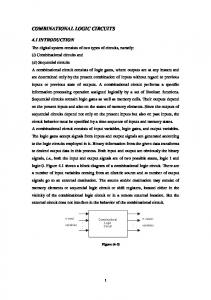
Fig. 1. Two combinational circuits implementing the same Boolean function.

Y X

root 1

X ! Y X X .0 !KL,Z6[]\GZN^`_baO,c:d ef^`_bagV If is an operator vertex, then YX is the function X h,c:d ef^`_bai2?'kjWZ6[l\GZN^m_nagV

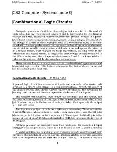
Clearly, BEDs are closely related to combinational circuits. Any Boolean circuit [5] can be transformed into a BED by replacing each input with the BED representing (a variable , , and ) and vertex with replace each -input gate by a tree of operator vertices encoding the Boolean function of the gate. This translation is clearly linear in size. Similarly, any BED can be converted to a circuit. Each variable occurring in the BED is an input to the circuit. An operator vertex is replaced by the corresponding gate, and a variable vertex with the sub-circuit , , , . This translation where is also linear. Thus, in terms of succinctness BEDs and combinational circuits are equally expressive. For instance, since there are combinational circuits implementing multiplication using only a quadratic number of gates [6], there also exists BEDs of this size representing them. To illustrate how BEDs are used to check the equivalence of two combinational circuits, consider the circuits in Fig. 1. To verify the equivalence of the two circuits, the BED for each circuit is constructed and the corresponding outputs are connected with biimplications, see Fig. 2 (the low-edges are drawn using dashed lines). We show that both roots of this BED are tautologies without constructing OBDDs for the two circuits by performing a case-split on the variable . (These steps are an approximation of how the algorithm UP _ ONE works; the details follow in Section III-B.) When is false, a simple evaluation of the BED according to Definition 2 yields that both outputs of the circuits have the value and thus the biimplication reduces to . In the other case, when is true, the BED is simplified but does not immediately reduce to the terminal . The BED from Fig. 2 after the case-split on variable is shown in Fig. 3. Thus, by moving to the top, we have shown that the outputs of the two circuits are identical for all input combinations with

t

J .0'op @245 !oqI

tQuwv

v

root 2

m

G

3

3

@

0

xUBJyRQz/,T{|JyR~}g J%-/.0! zs@2/45! }7A8:9*7f ! H

G

J 7'8:9-7f!rs

M

1

Fig. 2. The BED used in checking the equivalence of the two circuits in Fig. 1.

(notice that the low-edge of the variable vertex with points to ). The case where is proved by applying local reduction rules (these reduction rules are described in more detail in Section II-C) and identifying equivalent vertices (vertices with same operator, low- and high-child). This is shown in Fig. 4 and 5. Notice that the final OBDDs (the terminal ) for both roots are constructed without building the OBDDs for outputs and ( ). The efficiency of this way of transforming a BED into an OBDD is illustrated when verifying that two combinational 16-bit multipliers (c6288 and c6288nr from the ISCAS 85 benchmark) implement the same function. Using BEDs, the 32 outputs are shown to be identical in less than two seconds. Using OBDDs, this verification problem is infeasible due to the blowup of the OBDD representation whose size is exponential in the number of operand bits. Similar to OBDDs, the efficiency of the BED approach relies on a good variable ordering. We describe two ordering heuristics which seem to work well with BEDs. Using these heuristics, we report on the verification results for a large number of circuits (more than 250 circuits) from the ISCAS 85 and LGSynth 91 benchmarks. The results show that the BED ap-

v

BvNO

root 1

root 1

3

3

3

root 1

root 1

3

root 1

root 1

0

1

0

1

(a)

0

1

(b)

0

(c)

1 (d)

root 2

root 2

3

root 2

1

(e)

(f)

YmA#3£m¤0*¥W¢/¦¢*@#E o-¢ .. b) to c): Identify the two

@o¡wNE¢

Fig. 4. Steps used to show that root 1 from Fig. 3 is a tautology. a) to b) Use the identity . e) to f): Use the identity Identify the two vertices. d) to e): Use the identity

1

vertices. c) to d):

root 2

@

@

@ root 2

0

1 (a)

3o¡wNk§¢

0

1

0

(b)

3£`¤¥¢N¦¢*k§¢

(c)

Fig. 5. Steps used to show that root 2 from Fig. 3 is a tautology. a) to b): Use the identity . d) to e): Use the identity . the identity

proach performs extremely well for circuits that are structurally similar (sometimes several orders of magnitude faster than existing techniques) and is capable of verifying very large circuits (up to 104,000 gates) which have been drastically modified (using SIS [7] to reduce area). A. Related Work Current approaches for equivalence checking of combinational circuits can be classified into two categories: functional and structural. The functional methods consist of representing a circuit as a canonical decision diagram. Two circuits are equivalent if and only if their decision diagrams are equal (isomorphic). To

1

1

1

(d)

(e)

Y3fr@ ¦=U\]ÿ/=Q?Â^UYUó6ô!\]õ*_S`bö%aS`÷G_SõbcdóOø';>=e÷6\]öVW>f°?¨óOô!Xõ*W`¦Zö Y/ ç ç õ-û:ü õ&&í] îBì ýé6æêkú°DxDì ù@ì k6æù %ë Dìù@D6æù@¦ ¦ |ì ÿ!ù ë óOô!mõ-ÿéö ê0x ¦ù éJxù@¦ ù éJ´|ÿD¦ õ-û:ü õ&í] îBì ý 6æ ú°xDù@ì + 6æN Dìù@6æ¦ |ÿ!óOô!õ-ééö ê0ê0¦¦2ÿù éL>JMÿ'xDù@ù@¦¦ÿ/2ÿ L>¦ Mÿ'mÿxD õ-û:ü õMù éÿ'J´Dù@|ÿ¦Dÿx¦ éê0¦ùm¦2ÿ L MOÿ!|ÿDx ;>=f`:_SaExX W`S¦ Y/S¦ _=i? ÷õbóOø'÷6öË÷

APPLY

7

APPLY APPLY

(a)

Í 9 7

78

Î

Í

â/ã 9 7:8

Î

7

â/ã Í X

78

APPLY APPLY

9

Í 7 Î

APPLY APPLY

E

(b)

Fig. 11. Illustration of the up-step (a) for the case where variable exists in both children of the root and (b) for the case where only occurs in the left child.

G

Fig. 14. The APPLY-operation. Assumes and are OBDDs. The imposed total order on the variable vertices is denoted . In the code it is assumed that terminal vertices are included at the end of this order when comparing and . The memoization table must be initialized to empty prior to the first call.

ì 6æ xù@ ì 6æ mÿ

R

N

:õ-í îYû:ü ñUõ;>@í]=@ñ!îYkRwñ isóOô!a õ*terminal öÊ÷õnóOø'ó6÷6ô!öAõ*R%öÊ3÷Gñ°õb óOø'÷6ö#ñ õ-û:ü õ FEm¦GN- _ Dù éJ´Dë/D¦ _ |ÿ2L MOÿ!xëxD / jOE and G are OBDDs j / í][î E &and G ý areúN3þgterminal 5: vertices ó6ô!õ*ö x ë O ¦ m ù ¦ ÿ 6: 7: is a variable ´óOô!õ-ö * õ @ û ü õ ] í Y î g þ @ ! ñ 8: & ý 6æ úN K'¦ ùm¦ÿ6æ * õ @ û ü õ í]îfì xù@k%ì |ÿ!ó6ô!õ*ö 9: 10: & ý úNDì 6æ Dù@¦ _ ýý úN3þgxë¦Où éJ´xù@¦Gù éJ´|ÿDx¦ 6æ xù@+6æN ì 6æ |ÿ_!ó6ô!õ* ö ý úN3þgxë¦Gÿ2L MOÿ!xù@¦ÿQL MOÿ!mÿ/DDx 11: * õ @ û ü õ ] í f î ì ý & úNDì Dù@¦ _ ý úN3þgxë¦Où é J´xù@¦ÿD¦ 12: næ ý Dù@[g 6æì næ mÿ/kh _ ý úN3þgxë¦G2ÿ L MOÿ!xù@¦ÿ/DD 13: * õ @ û ü < õ ì & úNDì mÿ¦ _ ý úN3þgxë¦Oùm¦ù lé J´mÿxD¦ 14: úN3þgxë¦Oùm¦2ÿ L MOÿ!|ÿDxD _ 15: ;>=Qf`:_SaE3ñA¦Sn in R 16: ÷GõbóOø'÷6ö UP _ ALL

1: 2: 3: 4:

:õ-í îBû:ü @õ'3¦Dí]'îYñ!¦xis=@E ?a terminal óOô!õ-öo÷ó6õnô!ó6ø'õ*öÊ÷OöA÷Gõb?¨óOø'CBN÷6¦ö#D/ ñ õ-õ-û:û:üü õõ í]îWþg@ñ! is variable ióOô!õ-öË÷õnóOø'÷6öoñ @'with ¦ù éJì x6æëxDë/¦ O NP_ KóOô!õ-K!ö ¦ÿ2L MOÿ!xëxD _ í]FîWEm¦HþgGN&@Iñ! isý aú°variable 6æ ì þgDë/GN¦ ùmare¦ÿ both variable ´ó6ô!õ*ö õ*û@üõ&í] îWþgý E@ú° x and K!¦ ýý úN3þgDë/¦Où é J´Dù@¦ ù é J|ÿD¦ úN3þgDë/´óO¦Gô!2ÿ õ-L>Mö ÿ'Dù@¦2ÿ L>Mÿ'mÿxD * õ @ û ü õ ] í W î g þ ý E@ is variable 10: & ú° K!¦ ýý úN3þgDë/¦Où é J´Dù@¦ÿ¦ 11: úN3þgDë/´¦GóO2ÿ ô!L>õ-Mÿ'ö Dù@¦ÿx 12: * õ @ û ü õ ] í W î g þ ý GN is variable & ú° K!¦ ýý úN3þgDë/¦Oùm¦ù é J´|ÿD¦ 13: úN3þgDë/¦Oùm¦Qÿ L MOÿ!mÿ/DD 14: * õ @ û ü õ ý 15: & ú°`þgDë/¦ùm¦ÿ 16: insert x@'¦ñ°¦ 6 in R 17: ÷GõbóOø'÷6ö UP _ ONE

1: 2: 3: 4: 5: 6: 7: 8: 9:

UP ONE

UP ONE

UP ALL UP ALL

UP ALL UP ALL

R

R

C. Construction of OBDDs with U P _ ALL

An alternative way to construct an OBDD is to move all variables up simultaneously, called UP _ ALL. U P _ ALL is a generalization of Bryant’s APPLY-operator, shown in Fig. 14. Construction of OBDDs from a Boolean expression using recursive calls of APPLY suggests a bottom up conversion of BEDs into OBDDs. The UP _ ALL algorithm does that by moving all variables up as a block past the operator vertices. U P _ ALL is shown in Fig. 15. Let

µ

be a vertex in a BED and let

UP _ ALL

N

Fig. 15. The UP _ ALL-operation on OBEDs. The total order is defined as must be initialized to for APPLY (see Fig. 14). The memoization table empty prior to the first call.

Fig. 13. The UP _ ONE-operation. U P _ ONE takes an ordered BED as argument and returns an equivalent BED with pulled up as far as possible without violating the ordering. The imposed total order on the variable vertices is must be initialized to empty prior to denoted . The memoization table the first call.

N

UP ALL

UP ALL UP ALL

ñ

UP ALL

|µW . Then

UP _ ALL

has the following key properties:

| Y XÂ« Î . D is an OBDD. | If z and } are OBDDs, then APPLY G2O?;FO7E UP _ ALL y*®N¯b±g2*²N¯'2?b67kG . D' If z and } are OBDDs, the running time of } % . UP _ ALL 2?´b67k is /y$ % $z %F% m Properties D and DA make clear the relation between

UP _ ALL and APPLY . The time to build an OBDD bottom up using APPLY (the standard way) and building it from a BED using UP _ ALL is within a constant factor. Experiments have shown that the time to construct an OBDD using UP _ ALL is comparable to that of state-of-the-art OBDD packages and due to the operator reductions, it can be significantly faster. However, the worst-case runtime of UP _ ALL is exponential in % .% , but for the same reason as UP _ ONE, this is optimal.

µ

IV. VARIABLE O RDERING The efficiency of UP _ ONE and UP _ ALL depends on the variable order. Although the initial and final size of the BEDs are independent on the variable order when the two circuits implement the same function and thus the result is the tautology , the size of the intermediate BEDs depend on the ordering. A large number of variable ordering heuristics have been developed for OBDDs based on the topology of a circuit [33], [38], [39], [40], [41], [42], [43]. The heuristics attempt to statically determine a variable order such that the OBDD representation of the circuit is small. Typically, these heuristics consist of two steps to obtain a single global variable order: first, an order of the primary outputs is constructed, then for each of the primary outputs in this order, the variables in the support of the output are ordered. We only consider the second step (finding a variable order for a given primary output), since different variable orders can be used for different roots of a BED (see Fig. 10). This allows a greater flexibility to find good variable orders since the orders of the primary outputs are independent. However, the cost is that there is only limited reuse between verifying different primary outputs. Since UP _ ALL essentially works as an improved APPLY (property ), the variable orders that are good for OBDDs will also be good orders to use with UP _ ALL. Thus, when using UP _ ALL we can immediately use the variable ordering heuristics developed for OBDDs. Since UP _ ONE works quite differently than UP _ ALL, the variable ordering heuristics developed for OBDDs may not be effective when using UP _ ONE. However, our experiments show that this is not so; a good OBDD variable order also keeps the intermediate BEDs small when constructing an OBDD with UP _ ONE . The reason for this is that a good variable order for OBDDs has dependent variables close in the order. This allows UP _ ONE to collapse sub-circuits early in the verification process. Also, a good variable order has the variables that affect the output the most early in the order. U P _ ONE will then pull these variables to the root first which allows the most reductions. An example of this was the use of in the introductory example in Fig. 3. In the following we present two variable ordering heuristics, originally developed for OBDDs, which have proven to be effective for BEDs. A number of variable ordering heuristics are based on a depthfirst traversal of the circuit [39], [41], [42]. A depth-first traversal is a simple and fast heuristic that has shown to be practical for most combinational circuits [33], [39] since inputs that are close together in the circuit are also placed together in the ordering. The depth-first based heuristics differ in how they decide in what order the inputs of a gate are visited. The FANIN heuristic by Malik et al. [42] uses the depth of the inputs to a gate to determine in what order to consider the inputs. The depth of a terminal or variable vertex is and the depth of an operator vertex is n5oep q q Ur . The total runtime of FANIN to determine the variable order of s roots is / ts [42] where is the total number of reachable vertices from the s roots. The FANIN heuristic does not capture that variables affecting the output the most should be ordered first, something which

|

µ

y Ç

WG²N¯? |7B3245·g 6-²N¯? |7B7A8:9*7B ·E G q) Ç

is particularly important for UP _ ONE. The DEPTH _ FANOUT heuristic [43] attempts to determine the variables that affect an output the most by propagating a value from the output backwards towards the primary inputs. The value is distributed evenly among the input signals to a gate: if a value of u is assigned to the output of a gate with input signals, the value assigned to each of the fanin signals is incremented by u2v (the signal may be input to several gates and thus obtains a contribution from each gate). After propagating the value throughout the circuit to the primary inputs, the DEPTH _ FANOUT heuristic adds the primary input with the highest value to the variable order. This input is then removed from the circuit and the process is repeated until all variables in the support have been included in the variable order. The runtime of DEPTH _ FANOUT is / ws where is the total number of reachable vertices from the s roots and is the number of variables (inputs to the circuit). Thus, this heuristic takes slightly longer to compute than FANIN .

Ç

yxt Ç

Ç

Ç

t

Ç

DµY

V. E XPERIMENTAL R ESULTS In this section, we report the results from verifying a number of multi-level combinational circuits from the ISCAS 85 and LGSynth 91 benchmarks 2. The ISCAS 85 benchmark consists of eleven multi-level combinational circuits, nine of which exist both in a redundant and a non-redundant version. Furthermore, the benchmark contains five circuits that originally were believed to be non-redundant versions but it turned out that they contained errors and weren’t functionally equivalent to the original circuits [20]. The circuits in the ISCAS 85 benchmark are by some researchers considered too simple to use as benchmark circuits with todays technology. This may be true for some application areas but these circuits have several properties that make them suitable as benchmark circuits for evaluating techniques for performing a combinational logic-level verification. First, the circuits, although quite small, are not easy to verify both due to their functionality (for example, one of the circuits is a multiplier for which OBDD techniques fail) and due to a rather large logic-depth (up to 125 logic levels). Even with recent structural techniques, some of these circuits take more than an hour to verify [21]. Secondly, the circuits in the ISCAS 85 benchmark are ideally suited for testing logic-level verification techniques since they come in two functionally equivalent versions. To evaluate the BED technique on a broader and more realistic class of circuits, we also consider the 77 multi-level combinational circuits and the 40 sequential circuits from the LGSynth 91 benchmark. These circuits do not come in two versions, so instead we map each of the circuits to a gate library using SIS [7] and then optimize the circuits with respect to area. We then verify that 1) the mapped circuit corresponds to the original description, and 2) that the mapped and the optimized circuits implement the same functionality. Due to the nature of the mapping and optimization steps, the circuits differ in structure considerably more than the ISCAS 85 circuits. All experiments are carried out on a 300 MHz Pentium II PC running Linux. Verification approaches based on decision dia-

Ò

These benchmarks are available from The Collaborative Benchmarking Laboratory (http://www.cbl.ncsu.edu/)

grams typically run out of memory before running out of time. Thus, to demonstrate the effectiveness of BEDs, in all experiments we limit the memory consumption to 32 MB divided between 28 MB of memory to the node table (that is 1.46 million nodes corresponding to 20 bytes per node) and 4 MB to caches. The runtimes to determine the variable orders are insignificant (at most two seconds for any of the circuits) when using the FANIN heuristic. Using the DEPTH _ FANOUT heuristic it takes less then three seconds for the ISCAS 85 circuits, less than five seconds for the combinational LGSynth 91 circuits, and less than ten seconds for the sequential LGSynth 91 circuits except for the circuits s15850.1, s38417, and s38584.1 which take 33.7, 111.8, and 94.1 seconds, respectively. The times to determine variable orders are not included in the CPU times reported in the following, making a direct comparison between the different verification approaches possible. A. The ISCAS 85 circuits Table I shows the size of the ISCAS 85 circuits and Table II shows the runtimes to perform the equivalence check using BEDs. When using UP _ ONE, the DEPTH _ FANOUT heuristic

c432/nr c499/nr c499/c1355 c1355/nr c1908/nr c2670/nr c3540/nr c5315/nr c6288/nr c7552/nr

Inputs

Outputs

Gates

36 41 41 41 33 157 50 178 32 207

7 32 32 32 25 63 22 123 32 107

433 516 868 1204 2134 2603 3901 6018 4847 8067

A.1 Proving Non-Equivalence Table III shows the runtimes to determine non-equivalence of the erroneous ISCAS 85 circuits. The reported CPU times are for finding all errors. Although it does take longer to prove non-equivalence, as expected since less equivalences exist, the increase in the runtimes is insignificant. TABLE III RUNTIMES ( IN CPU SECONDS ) FOR SHOWING NON - EQUIVALENCE OF THE REDUNDANT AND NON - REDUNDANT CIRCUITS IN THE ISCAS 85 BENCHMARK .

TABLE I S IZE OF THE ISCAS 85 BENCHMARK CIRCUITS . Circuit

there is little difference between the two ordering heuristics when using UP _ ALL. The performance of UP _ ONE and UP _ ALL is comparable except for the circuit c6288 where only UP _ ONE succeeds. This circuit implements a 16-bit multiplier for which it is known that the OBDD representation grows exponentially [3]. The OBDD representation of a 16-bit multiplier uses more than 40 million vertices [44] and this number is approximately 2.7 times larger for each additional bit in the operands. Thus, UP _ ALL will fail on this circuit no matter what variable ordering is used. In contrast, UP _ ONE never builds the OBDD representation of the multiplication function and thus the circuits can be verified in just a few seconds.

Circuit

# errs. 1 6 5 33 28

c1908/nr_old c2670/nr_old c3540/nr_old c5315/nr_old c7552/nr_old

U P _ ONE FANIN D ._ F. 1.0 6.5 26.6 29.1 7.0

1.0

x

23.3 4.3 8.7

U P _ ALL FANIN D ._ F. 1.0 1.3 17.3 3.6 2.9

1.0

x

27.9 3.5 3.6

A.2 Effect of Operator Reductions TABLE II RUNTIMES ( IN CPU SECONDS ) FOR VERIFYING EQUIVALENCE OF THE REDUNDANT AND NON - REDUNDANT CIRCUITS IN THE ISCAS 85 BENCHMARK . F OR EACH PAIR OF CIRCUITS , THE TIME IS GIVEN WHEN USING THE TWO DIFFERENT VARIABLE ORDERING HEURISTICS FANIN AND DEPTH _FANOUT ( ABBREVIATED D ._ F.) AND USING THE TWO DIFFERENT

BED INTO AN OBDD, UP _ ONE AND T HE BEST RUNTIMES ARE HIGHLIGHTED USING BOLDFACE . A

ALGORITHMS FOR TRANSFORMING A UP _ ALL .

x

‘ ’ REPRESENTS THAT THE VERIFICATION FAILED DUE TO LACK OF MEMORY.

Circuit c432/nr c499/nr c499/c1355 c1355/nr c1908/nr c2670/nr c3540/nr c5315/nr c6288/nr c7552/nr

U P _ ONE FANIN D ._ F. 2.5 5.2 1.6 5.3 1.0 1.4 16.9 17.8 2.0 4.6

U P _ ALL FANIN D ._ F.

2.2 2.6 1.6 2.6 1.0 1.2 21.8 3.1

2.1 2.4 1.6 2.6 1.0 1.0 17.0 3.1

2.2 2.6 1.6 2.6 1.0 1.0 33.7 3.1

3.7

2.6

2.6

x

x

generally computes a better variable order than

z

x

FANIN ,

To illustrate the effect of operator reductions, we repeat the experiments in Table II and III but without performing any of the operator reductions described in Section II-C. The only reductions performed are those required to maintain reducedness, see Definition 1. The operation of UP _ ALL then reduces to that of APPLY, that is, the performance of UP _ ALL corresponds very closely to that of APPLY in a reasonable implementation of an OBDD package. The results are shown in Table IV. Clearly, the efficiency of UP _ ONE relies heavily on the operator reductions to identify identical nodes in the BED and thus avoiding to transforming them into OBDDs. Without reductions, a large number of the circuits cannot be verified (with 32 MB of memory) and the runtimes for those that do succeed are up to several orders of magnitude longer. When using UP _ ALL the situation is quite different. In building an OBDD using UP _ ALL, any vertex that is constructed during the transformation will have non-operator vertices as the is called in the body children. I.e., whenever of UP _ ALL, both and are variable or terminal vertices. Thus, the operator reductions only affect the performance of UP _ ALL by reducing the initial size of the BED. For some circuits (e.g., c3540) this initial reduction has a large impact on the runtime

while

}

y*®N¯b±g2*²N¯'x³iFO7E

y

TABLE IV RUNTIM ES ( IN CPU SECONDS ) FOR VERIFYING EQUIVALENCE OF THE REDUNDANT AND NON - REDUNDANT CIRCUITS IN THE ISCAS 85 BENCHMARK WITHOUT PERFORMING OPERATOR REDUCTIONS .

Circuit c432/nr c499/nr c499/c1355 c1355/nr c1908/nr c2670/nr c3540/nr c5315/nr c6288/nr c7552/nr c1908/nr_old c2670/nr_old c3540/nr_old c5315/nr_old c7552/nr_old

U P _ ONE FANIN D ._ F. 2.9 166.1 532.5 743.5

x

x

x

15.3 29.0 4.8

2.5 2.5 3.9 4.1 1.0 1.4 56.9 3.5

7.4

7.2

3.1

3.7

x

14.9

1.0 1.5 60.4 4.0 3.1

1.0

x

2.6

U P _ ALL FANIN D ._ F.

x x x x

111.7

x

116.4

x

10.0

x x x

6.0 15.2

x

2.3 4.1 4.8 4.8 1.0 1.9 145.4 3.3

x x

126.4 3.7 4.1

of UP _ ALL. This experiment indicates that performing an initial operator reduction step, as discussed in the introduction, can improve the time to construct an OBDD. B. The LGSynth 91 Benchmarks By construction, the redundant and non-redundant versions of the ISCAS 85 benchmark circuits have many structural similarities and are thus ideally suited for the BED approach. To test the verification strategy on a broader range of circuits with fewer structural similarities, we consider the circuits from the LGSynth 91 benchmark. This benchmark includes 77 multi-level combinational circuits and 40 sequential circuits. These circuits are mapped to a gate library (msu.genlib) using SIS and then optimized for area using the SIS script script.algebraic. As mentioned above, there are two verification problems: one is to verify that the original circuits correspond to the mapped versions and one is to verify the mapped versions against the optimized versions. Due to the nature of the mapping and optimization steps, the circuits differ in structure considerably more than the ISCAS 85 circuits. The results for the 77 combinational circuits are shown graphically in Fig. 16. The eleven ISCAS 85 circuits are included in the LGSynth 91 benchmark and although some of the LGSynth 91 circuits are considerably larger than the ISCAS 85 circuits, the ISCAS circuits are the most difficult ones to verify using the BED approach. The mapping of each circuit is verified in less than three minutes. The results for the verification of the optimization step are similar, except that the verification of the optimization step of C6288 failed using both UP _ ONE and UP _ ALL. The results for the verification of (the combinational portion of) the 40 sequential circuits in the LGSynth 91 benchmark are shown in Fig. 17. The mapping of the traditionally difficult circuit s38417 takes 20 minutes to verify and the verification of mm9b fails for both variable ordering heuristics. The mapping of the remaining 38 circuits is verified in less than one minute. The optimization of each circuit, except for mm9b and s38417, is also verified in less than one minute. The verification of mm9b

and s38417 both fail when using 32 MB of memory. Using 64 MB of memory, s38417 is verified in an hour using the FANIN ordering heuristic. The circuit mm9b is an instance where the two ordering heuristics fail to construct a good variable order, thus the verification of both the mapping and the optimization steps fail, even when using 64 MB of memory. Using the order in which the variables appear in the specification, the mapping of mm9b is verified using 64 MB of memory in 207 seconds and 270 seconds using UP _ ONE and UP _ ALL, respectively. Similarly, the optimization of mm9b is verified in 69 seconds and 115 seconds using UP _ ONE and UP _ ALL, respectively. C. Comparisons of Results The ISCAS 85 benchmark has been used extensively by researchers to test techniques for solving the equivalence problem. Since all researchers have solved the exact same verification problems, there is a good basis for comparing the different approaches. Table V shows the runtimes to verify the ISCAS 85 circuits using recent methods. The experiments are carried out on different machines and are therefore not directly comparable. However, the efficiency of the machines only differ by a small constant and not by orders of magnitude and therefore the comparisons still give a good indication of the relative virtues of the different approaches. The experiments of Brand [18] is an exception since he does not report runtimes for comparing the redundant and the non-redundant versions. Instead the circuits are synthesized and optimized, much in the same way as we have done for the LGSynth 91 circuits. This might well be a more difficult verification problem. From Table V it is clear that the learning-based approaches [21], TABLE V RUNTIMES ( IN CPU SECONDS ) OF OTHER APPROACHES FOR VERIFYING THE ISCAS 85 BENCHMARKS . N OTICE THAT THE RESULTS OF B RAND [18] ARE NOT DIRECTLY COMPARABLE SINCE A DIFFERENT VERIFICATION PROBLEM IS SOLVED . “ N / A” DENOTES THAT THE RUNTIME HAS NOT BEEN REPORTED . Circuit

BED

[18]

[21]

[22]

[24]

[26]

[45]

c432/nr c499/nr c1355/nr c1908/nr c2670/nr c3540/nr c5315/nr c6288/nr c7552/nr c1908/old c2670/old c3540/old c5315/old c7552/old

2.1 2.4 2.5 1.0 1.0 16.9 3.1 2.0 2.6 1.0 1.3 17.3 3.5 2.9

4.0 38.0 9.0 22.0 58.0 39.0 29.0 193.0 136.0 n/a n/a n/a n/a n/a

1.0 1.9 6.6 11.2 159.3 67.6 372.8 21.5 5583.3 n/a n/a n/a n/a n/a

2.0 5.0 20.0 22.0 61.0 281.0 190.0 40.0 412.0 n/a n/a n/a n/a n/a

0.8 1.2 3.4 6.2 3.9 17.4 14.0 9.1 20.6 n/a n/a n/a n/a n/a

0.2 0.2 0.5 1.6 0.8 3.0 2.7 4.3 34.6 2.5 54.6 2.9 8.3 26.2

0.4 0.4 1.0 2.1 3.4 12.7 8.3 7.2 20.8 n/a n/a n/a n/a n/a

[22] are inefficient for larger circuits. The runtimes of the BED approach is generally comparable to (and sometimes better than) the other three approaches [24], [26], [45]. Moreover, these runtimes should be seen in the light of the fact that the BED experiments only use 32 MB of memory. Only van Eijk [26] has reported runtimes for the erroneous ISCAS 85 circuits. For these circuits it is observed that the BED

¥£