Equivalence Hypothesis Testing in Experimental Software ...

Sofware Quality Journal manuscript No. (will be inserted by the editor)

Equivalence Hypothesis Testing in Experimental Software Engineering Jos´ e Javier Dolado · Mari Carmen Otero · Mark Harman

Received: date / Accepted: date

Abstract This article introduces the application of Equivalence Hypothesis Testing (EHT) into the Empirical Software Engineering field. Equivalence (also known as bioequivalence in pharmacological studies) is a statistical approach that answers the question ‘is product T equivalent to some other reference product R within some range ∆?’. The approach of “null hypothesis significance test” used traditionally in Empirical Software Engineering seeks to assess evidence for differences between T and R, not equivalence. In this paper we explain how EHT can be applied in Software Engineering, thereby extending it from its current application within pharmacological studies, to Empirical Software Engineering. We illustrate the application of EHT to Empirical Software Engineering, by re-examining the behaviour of experts and novices when handling code with side effects compared to side effect free code; a study previously investigated using traditional statistical testing. We also review two other previous published data of software engineering experiments: a dataset compared the comprehension of UML and OML specifications and the last dataset studied the differences between the specification methods UML-B and B. The application of EHT allows us to extract additional conclusions to the previous results. EHT has an important application in Empirical Software Engineering, which motivate its wider adoption and use: EHT can be used to assess the statistical confidence with which we can claim that two software engineering methods, algorithms of techniques are equivalent. The data, R scripts and other information is available at http://www.sc.ehu.es/jiwdocoj/eht/eht.htm. JJ Dolado Facultad de Inform´ atica, UPV/EHU Univ. of the Basque Country, Spain. E-mail: [email protected] MC Otero Escuela Universitaria de Ingenier´ıa de Vitoria-Gasteiz, UPV/EHU Univ. of the Basque Country, Spain. E-mail: [email protected] M Harman CREST, University College London, WC1E 6BT, UK. E-mail: [email protected]

2

Jos´ e Javier Dolado et al.

Keywords Equivalence Hypothesis Testing · Bioequivalence Analysis · Program Comprehension · Side-effect Free Programs · Crossover Design · Experimental Software Engineering

1 Introduction One of the main concerns in any experimental or empirical research work is to provide evidence that the conclusions we infer from the quantitative data obtained in experimentation are valid and of practical use. The goal of any statistical procedure in empirical research is to seek to exclude chance from the conclusions that will be attributed to the substantial hypotheses on which we base our scientific claims. The approach that is usually followed in empirical software engineering experiments takes the form of testing, by some statistical procedure, the null difference between the means of two populations: µT , the mean of the new treatment, and µR , the mean of reference. This is called “Null Hypothesis Significance Test” (NHST). The goal is to be in a position to reject the hypothesis of no difference H0 , in order to accept the alternative hypothesis of difference, Ha , i.e.: H0 : µ T − µ R = 0 Ha : µT − µR 6= 0 for the two-tailed test

(1)

The reasoning process is based on the standard theories of Fisher and NeymanPearson. For accepting or rejecting H0 , software engineers use the p-value of the test and typically seek to reduce the chances of committing so-called Type I and Type II errors. The original null hypotheses of Fisher and the two other authors Neyman and Pearson have different interpretations concerning the burden of proof relating to the p-value or the Type I or II errors. The general procedure (occasionally mixing both approaches) has been followed with increasing frequency, and perhaps with a certain degree of ritual, in the Empirical Software Engineering literature. In this paper we present the rationale for an alternative method to Null Hypothesis Significance Test (NHST) called Equivalence Hypothesis Testing (EHT). Our goal is not to replace the use of NHST. Rather, we wish to introduce to the Empirical Software Engineering community the concepts and practice of EHT, which is currently more widely seen in pharmacological studies (where it is often referred to as the ‘bioequivalence testing’ since it assesses the evidence that one drug treatment has equivalent biological effects to another). Our motivation for introducing EHT is twofold: 1. To Complement NHST: Where we have evidence from NHST that two populations of results are different, we can use this to assert that we have statistical evidence for scientific claims about the populations. However, EHT allows us to explore the results in more detail. It gives us additional insights into the effect size and the confidence with which we may assert differences over ranges of effect size, by examining the equivalence intervals. This is often important because knowing that two software engineering methods behave differently is only a starting point for actionable results; we also need to know, for example, how confident we can be that the effect size is worthy of action.

Equivalence Hypothesis Testing in Experimental Software Engineering

3

2. To answer Equivalence questions NHST cannot address: In software engineering empirical studies, we often would like to explore the confidence with which we can claim that two software engineering methods, algorithms or techniques are equivalent. For example, suppose we have two test data generation techniques (Lakhotia et al, 2009). We may believe that one achieves better test effectiveness for the same effort. We therefore would like to provide evidence to support our claim that the two techniques require equivalent effort. Alternatively, in source code analysis (Harman, 2010), we may have a performance improvement for some algorithm and we wish to show that the performance improvement does not affect the algorithm’s precision. That is we wish to show that the two versions of the algorithms have ‘equivalent precision’. In these situations authors are often tempted to use NHST to explore equivalence. However, failing to reject the null hypothesis in NHST is most definitely not the same as demonstrating equivalence; absence of proof (of difference) is not proof of absence.

In this paper we introduce EHT for empirical software engineers and explain how it can be used in Experimental Software Engineering work. As with NHST, the application of EHT to human-based empirical studies requires more care and attention because of the learning effects and other confounding factors that can affect the results of human studies. Fortunately, EHT is well-understood from its application to biological (pharmacological) studies where these issues are unavoidable. Therefore, there is a wealth of accumulated knowledge on which we can draw when extending EHT testing to empirical software engineering. In order to illustrate the application of EHT in Experimental Software Engineering, we chose a study of a software engineering problem that involved the performance of human subjects in cognitive tasks, since this exposes more of these issues. We also chose to study a problem for which EHT is used as a complement to NHST, since this will be the starting point for many software engineers who are already familiar with NHST. Thus, our illustration of EHT represents the more demanding case; the one that requires most additional statistical care and attention and ‘due diligence’ requirements on the experimentors. For those software engineers interested in using EHT to test equivalence of algorithms (where no humans involved), the techniques can be used with fewer additional requirements, making it simpler and easier to use EHT for Experimental Software Engineering. The rest of this paper is organised as follows. Section 2 introduces EHT for software engineers. Section 3 shows how to apply the EHT methods to software engineering problems. Section 4 details the type of experimental designs that can be used for EHT where human subjects are involved. Section 5 discusses the issue of sample size. Section 6 presents the analysis of the program comprehension experiment as an illustration of EHT for Empirical Software Engineering. Section 7 shows the application of EHT to two additional research problems and Section 8 discusses related work on the use of NHST and EHT. Finally, the Conclusions state the benefits obtained through the analysis of the data by EHT.

4

Jos´ e Javier Dolado et al.

2 Equivalence Hypothesis Testing Different terms are used for ‘equivalence’ in statistical procedures, such as bioequivalence, parity, equality and similarity. They are used for describing a situation in which two variables differ by less than a predetermined range (Ennis and Ennis, 2010). When comparing experimental data of two samples T and R, we may perform statistical tests for differences (NHST), for equivalence and for non-inferiority. In NHST, when we perform a difference test on a data set the result can be that we do not reject the null hypothesis of ‘no difference’ or that the H0 is rejected. In the last situation the new treatment T can be better or worse than R. Equivalence analysis differs from the classic t-test, partly because the goal is to establish whether the two treatments are the same. The null hypothesis is therefore that the mean responses are different and the alternative hypothesis is that the mean responses are equivalent. This way of proceeding is the opposite of the more usually applied null hypothesis of NHST. In EHT the parameters α (the Type I error), β (the Type II error) and the statistical power of NHST are also used, but with different meaning. Bioequivalence is the application of EHT ideas in the pharmaceutical field, where the usual aim is to compare the effect of two drugs, one being a generic product considered for introduction as a cheaper replacement for another, more expensive, proprietary drug. The goal of bioequivalence testing is to determine whether the new generic drug, T , can replace the existing drug R. It is advisable, therefore, to administer either the product or the treatment to the same subjects. The literature in bioequivalence speaks about superiority trials when the aim is to check whether a new treatment is better than the reference treatment, by using the NHST superiority tests, which correspond to equations (1) in Section 1. In a noninferiority trial (NIHT), the research question is whether T is no worse than a reference treatment R (Piaggio et al, 2006). Usually, a value ∆ is set for allowing small differences to the reference treatment. In a non-inferiority test the null and alternative hypotheses are H0 : µT − µR ≤ ∆ H a : µT − µR > ∆

(2)

where ∆ determines the range within which we consider that treatment of method T is noninferior to R. Equivalence trials are similar to noninferiority but the equivalence is defined between an interval +∆ and −∆ (Wellek, 2010). The null and alternative hypotheses are expressed as H0 : |µT − µR | ≥ ∆ (3) Ha : |µT − µR | < ∆ where ∆ determines the range within which we consider that treatment of method T is equivalent to R.1 Figure 1 shows the results that can be observed after the comparison of methods T and R, plotting the possible situations of the confidence intervals with 1 Although it is a rare situation, it is feasible to test for equivalence with the null hypothesis as H0 : |µT − µR | ≤ ∆. However, this procedure is rarely used in practice, since it does not allow to control for the “risk of the consumer” (Hauschke et al, 2007, pp. 45-46) therefore rendering the testing for equivalence useless. See (McBride, 2005, section 5.3) and (Cole and McBride, 2004) for the practical consequences of this approach.

Equivalence Hypothesis Testing in Experimental Software Engineering

New method T worse than R

5

New method T better than R

Area of Non-inferiority of T Equivalence Interval -Δ,+Δ Nonequivalent; Inferior

A

Nonequivalent; Inconclusive

B

Equivalent; Noninferior

C

Equivalent; Noninferior

D

Equivalent; Superior

E Nonequivalent; Superior

F Nonequivalent; Superior

G

Nonequivalent; Noninferior Inconclusive; Inconclusive Nonequivalent; Inconclusive T Worse

K

-50%·μR

-Δ

-20%·μR

I J

Nonsignificant

T Better

L

0 μT- μR

H

20%·μR

Δ

M

50%·μR

Fig. 1 Forest plot of the possible confidence intervals (CIs) A to J, with reference to the interval equivalence ±∆. The intervals A to J can be computed also for noninferior analysis. The dotted intervals K to M are the possible CIs in NHST.

respect to ∆. For illustration, the value of the interval ∆ is set between ±20% and ±50% around the null difference of the means, µT − µR , but its actual value must be set by the experimentor. When applied to pharmacological studies, the Type I error (falsely rejecting H0 when it is, in fact true, P (reject H0 |H0 )) is controlled by α and is referred to as the “risk of the consumer”, since it represents the risk of taking a drug or undergoing a treatment believed to be equivalent, when in fact it is not. The Type II error (falsely accepting H0 ) is controlled by β, P (not reject H0 |Ha ), and is referred to as the “risk of the producer” since the commercial firm may fail to recoup investment by deciding not to produce a drug, despite it actually being equivalent to the reference; Power is P (accept Ha |Ha ). The values of α and β represent the risks that the consumer and producer, respectively, are willing to take. For instance, should we decide to set α to be 0.1 then we assume that we may be using a method or product that we believe to be equivalent, when in fact it is not equivalent 1 in 10 times. If we set β at 0.2 we assume that we may be

6

Jos´ e Javier Dolado et al.

using a method or product that we believe it is inequivalent, when in fact it is equivalent 2 in 10 times. In EHT the goal is to check whether a method T is equivalent to R within a range ∆. Similarly to NHST, confidence intervals can be computed for testing equivalence or, alternatively, two simultaneous one-side tests can be used. The implications of these tests are presented in Table 1, which considers both NHST and EHT. Figure 1 shows the different possibilities and decisions based on our equivalence hypotheses. For example, segment C in the figure represents a confidence interval for the mean differences between T and R which is within the equivalence interval ∆ and which is also within the range of noninferiority to the reference R. The same segment C is classified in Table 1 as statistically different since it does not include the value 0. When using NHST we may obtain the CI L which does not reject the null hypothesis of non difference, but that would be classified as “equivalent” since it lies within the limits of the equivalence interval. Figure 1 and Table 1 help to make a decision about the treatment method T versus the reference method R. Table 1 Classification of the CIs of Figure 1.

XXX

NHST XX XX X

Statistically Different

Statist. Nonsignificant

Statistically Equivalent

C, E, K

D, L

Statistically Not Equivalent

A, B, F, G, M

H, I, J

EHT

3 Basic Procedures in EHT There are different methods for testing average equivalence between the difference of a mean of reference, µR , and a mean of a treatment, µT (Rani and Pargal, 2004) (Ennis and Ennis, 2009) (Chow and Liu, 2009) (Wellek, 2010) (Chen and Peace, 2011). Most statistical software packages have implementations of these methods. In the simplest approach they can be categorized as those based on testing a null hypothesis around an equivalence region and those based on using confidence intervals. Compared to NHST, the EHT null hypotheses are reversed and, correspondingly, the burden of the proof, the interpretation of the types of errors and the parameters (see Table 2).

3.1 Procedures based on Hypothesis testing The null hypothesis for EHT stated in equation 3 can be made operational in an interval hypothesis as follows (Chow and Liu, 2009) H0 : µT − µR ≤ −∆ or µT − µR ≥ +∆ versus Ha : −∆ < µT − µR < +∆

(4)

Equivalence Hypothesis Testing in Experimental Software Engineering

7

Table 2 Comparison of Type I and II errors in classical NHST, Equivalence (EHT) and Non-inferiority (NIHT). Type I error or False Positive. Reject H0 (α)

Type II error or False Negative. Not Reject H0 (β)

Burden of Proof

NHST

Concluding that R and T are different, when in fact they are not.

The alternative hypothesis of difference of R and T.

EHT

Concluding that R and T differ by less than ∆ when in fact they differ by ∆ or more.

NIHT

Concluding that T is non-inferior to R when in fact it is inferior.

Concluding that R and T are equal when in fact they are not. The alternative hypothesis Ha is rejected. Concluding that R and T are inequivalent in the interval −∆ and + ∆ when in fact they are equivalent. Concluding that T is inferior to R when in fact it is non-inferior.

The alternative hypothesis of equality by less than ±∆.

The alternative hypothesis of non-inferiority of T respect to R by ∆.

The best known procedure for hypothesis testing is known as TOST (two onesided t-tests) and is Schuirmann’s proposal (Schuirmann, 1987). It consists of decomposing H0 into two separate hypothesis and applying t-tests as follows H01 : µT − µR ≤ −∆ or H02 : µT − µR ≥ +∆ versus Ha1 : µT − µR > −∆ and Ha2 : µT − µR < +∆

(5)

The procedure tries to reject both H01 and H02 for infering equivalence. Also, as shown by (Ennis and Ennis, 2009), there is a possibility of directly testing equivalence with only one null hypothesis and other alternative hypothesis. There are different critics and variations on this type of hypothesis testing and to the different methods used (Ennis and Ennis, 2010), but it has been used extensively in the pharmacological area. Figure 2 shows graphically the two alternative hypothesis H01 and H02 in TOST versus the alternative Ha (Ha1 and Ha2 ). The graphs show the areas corresponding to the parameters α and β/2 used in the significance tests.

3.2 Procedures based on Confidence Intervals Confidence Intervals (CIs) can also be used for EHT and is the preferred method. The underlying idea in this procedure is to compute a (1 − 2α)100% statistical confidence interval around the sample mean differences, µ ¯T − µ ¯R , and to observe if it lies within the equivalence region previously defined. One of the basic criteria for setting the equivalence region is to use 20% around the known reference mean, µ ¯R , implying that the confidence interval for the difference must lie be between −0.2¯ µR and 0.2¯ µR (see subsection 3.4). From the practical viewpoint, the use of TOST with an α significance level is equivalent to using a CI of 1 − 2α (Chow and Liu, 2009). As the CI of the difference test is (1 − α), it contains the CI of the equivalence (1 − 2α). We can

8

Jos´ e Javier Dolado et al.

CI1 CI2

Accept Ha (equivalence)

Accept H01

Ha

H01

-Δ

β/2

-zα

α

0

Accept H02

H02

α

zα

β/2

Δ

μT- μR

Fig. 2 Plot of the TOST and the confidence intervals CI1 and CI2 for the difference of means.

summarize that whilst in NHST the CIs are computed with (1 − α), in EHT they are computed with (1 − 2α) and in NIHT they are computed with (1 − α/2). In Figure 2 we see above the TOST two potential CIs and their relationship to the interval equivalence. Visually, it is easy to spot that, in this case, CI1 is equivalent and CI2 is not. The CI expresses the confidence level, at a chosen %, that the computed interval will contain the true value of the difference of the parameter µT − µR , in the long run. As larger is the confidence level as larger will be the width of the CI since it has to include a larger set of plausible values. The most common method used for computing the CIs is the so called “Shortest Interval”. The limits for the Shortest interval (L, U) for the differences of the means are computed as

r (L, U ) = (µT − µR ) ± t(α, n1 + n2 − 2)ˆ σd

1 1 + n1 n2

(6)

where µT and µR are the sample means, σ ˆd is an estimation of the intra-subject variance, n1 and n2 are the number of experimental units in the two groups and t(α, n1 + n2 − 2) is the percentile of the t-distribution (Chen and Peace, 2011, pp. 263-265). Other usual alternative is to use Westlake intervals, that are symmetric (Westlake, 1976) but wider than the corresponding Shortest. A recent review of the different types of equivalence tests can be found in (Meyners, 2012).

Equivalence Hypothesis Testing in Experimental Software Engineering

9

3.3 Meta-analysis and EHT Meta-analysis is a statistical procedure that allows to integrate the results of a set of studies related to the matter of interest. This means that, given a series of experiments related to a subject of interest but separated in space and in time, such as the effect of a drug in the body, meta-analysis tries to reach a conclusion about the parameters of interest used in the studies. The goal is to combine the information for estimating the main values of the measures of effect, called effect sizes. There are different variables that reflect the effect sizes depending if they are based on means, proportions or correlation between measures. In traditional hypothesis testing one of the most common approaches to metaanalysis uses the means: the inferences are made for the absolute difference of the means and standardized mean difference and the confidence intervals around the mean of the whole set of studies are generated. Similarly to what is done in difference testing, meta-analysis can also be performed with EHT, but there are few works in the literature that deal with the issue. The known approaches are described in Chapter 16 of (Chow and Liu, 2009). We use Chow and Liu’s approach by computing the limits of the confidence interval (1 − 2α)100% for equivalence with meta-analysis as follows (L, U ) = d¯ ∓ t(α,

H X

q ¯ d (d) (nh1 + nh2 − 2)) Var

(7)

h=1

q ¯ is an estimate d (d) where d¯ is the combined estimate for µT − µR , and Var for the weighted intra-subject variance, being H the number of studies involved in the computations.

3.4 Limits for Equivalence or Practical Significance A key element in the application of EHT is the setting of the intervals of equivalence. These levels depend on the field of application and on the type of intervals that are being computed. Establishing these levels forces the analyst to set the ranges of practical importance of the differences in their respective field. The decision rule is thus simply to check whether the computed CI is included in the equivalence range. The pharmaceutical and medical fields have agreed on different levels that drugs have to fulfill to be considered equivalent. One of the earliest criterion used by the FDA, that has already been replaced by the ratio on different measures of the reference and the treatment, was to use the 20% of the reference means (Chow and Liu, 2009, p. 602). The European Medicines Agency, and similar regulatory bodies in the world, have established different levels for establishing the bioequivalence between two drugs (EMA, 2010). These are the leading areas where the bioequivalence methods have advanced since they are centered on the “risk of the consumer”. But there are other areas where equivalence limits have been explored and discussed taking into account the characteristics of the objects under study. In the ecologial modelling field Robinson and Froese explored different levels for equivalence using 10%, 25% and 50% relative to the sample standard deviation of the differences (Robinson and Froese, 2004, p. 355). In (Robinson et al, 2005) the

10

Jos´ e Javier Dolado et al.

authors chose arbitrarily a ∆ of 25% on the measures of interest (intercept and slope of a regression). In a work in the marine ecology field the limits were set at 50% of the standard deviation from the reference mean (Cole and McBride, 2004). Since there are no guidelines in our field we will provide two limits at 20% and at 50% over the means difference. In a recent software engineering study about traceability recovery (Borg and Pfahl, 2011), the authors chose to use an absolute interval of 0.05 for their specific analysis, which is not transferable to other settings (additional comments in Section 8).

4 Experimental Designs for Equivalence Studies Involving Human Subjects When comparing a method T respect to another method R, by using two groups of human subjects, the two basic designs to use are a crossover design and a parallel design. In a parallel design the experimental units are split into two groups and each group receives only one treatment. On the contrary, in a standard 2x2 crossover design, the experimental units receive each treatment, T and R alternatively. The advantages of a crossover study is that each group receives both treatments but in reverse order, i.e, a group receives the sequence of treatments RT and the other receives the sequence TR. The main benefit from the 2x2 crossover (RT/TR) is that it allows intra-subject comparison, since each subject receives both treatments. The crossover design is the design most used for bioequivalence studies, although a parallel group design can also be preferred in cases of long-life drug studies. Usually, the researchers want to know if a generic medicine can be exchanged by another original specific medicine and, hence, the appropriate design is a crossover (2 periods and 2 sequences of treatment). Two doses of medicines are bioequivalent if they produce the same therapeutic effect. There are several alternative designs such as a three period with two sequences with replication of R (RTR/TRR) or with replication of T (TRT/RTT), and a partial-replicate design (TRR/RRT/RTR) with three period with three sequences (Hyslop and Iglewicz, 2001) (Siqueira et al, 2005). In section 6 we will see that we have used a standard crossover (RT/TR) since our data fits with the characteristics of the standard analysis, which is a comparison of methods in which carryover and period effects may appear. In order to keep the analysis homogeneous, the two other datasets analysed in this work also use a crossover design (see Section 7).

5 Sample Size The sample size is an important parameter in both NHST and EHT procedures because its relationship to power (1 − β), i.e, the ability to correctly reject H0 (or to accept Ha ). Sample size increases the precision of the confidence intervals and the parameters of interest and decreases the amount of the sampling error. Sample size should be as large as possible in order to maximize power, since α is fixed. Ideally, the identification of the sample size, the effect size and the desired power is a requirement before conducting the experiment. However, there are many circumstances which make it difficult to provide the ideal initial analysis and, in

Equivalence Hypothesis Testing in Experimental Software Engineering

11

practice, one has to deal with less clear situations. In many occasions the sample size is fixed and/or the effect size has a wide range of variation.

5.1 Sample size for the Equivalence Hypothesis Testing Computing the sample size for equivalence requires different procedures from the NHST case (Chow and Wang, 2001). A description of the basic ways of computing sample size for bioequivalence can be found in (Chow and Liu, 2009). The work of (Piaggio and Pinol, 2001) describes the use of different parameters for computing sample size in reproductive health clinical trials and (Stein and Doganaksoy, 1999) computes sample size for comparing process means. The articles of (Rogers et al, 1993) and (Cribbie et al, 2004) explain how to compute sample size for using the Schuirmann’s test of equivalence and compare it with the traditional t-test. Finding the exact sample size in TOST requires the numerical integration of the t distribution with some specific parameters (see (Chow and Liu, 2009), sec. 5.3). From (Chow and Liu, 2009) we show here the simplest approach for computing sample size, which is to take the interval hypothesis (i.e, equations (4) for reference mean and a 20% interval around it). Power is set at 80%. This sample size can be computed manually as follows: ne ≥ [t(α/2, 2n − 2) + t(β, 2n − 2)]2 [CV /20]2

(8)

where t(α, ν) is the α-th percentile of a t-distribution with ν degrees of freedom, being the total number of√ subjects N = 2n. CV is the coefficient of variation, SE defined as CV = 100 × M and M SE is the mean square error from the µ ¯R analysis of variance table for the standard 2x2 crossover design. It is evident that both M SE and µ ¯R should be known in advance or a value should be assumed. Therefore these procedures serve the purpose of verifying the sample size actually used. Finally the value of ne is computed through iterations until the inequality is met. The requirements of sample size are higher in EHT than in NHST, for obtaining the same power. This behaviour was described by (Siqueira et al, 2005) (Ogungbenro and Aarons, 2008) (Cribbie et al, 2004) (Tempelman, 2004). (Ogungbenro and Aarons, 2008) used simulations for determining sample size in the confidence interval approach to equivalence. (Siqueira et al, 2005) explored a set of sample size formulas and concluded that when there is high variance a 2x2 crossover requires large sample sizes to achieve a reasonable power for testing bioequivalence. In NHST, generally, sample size is directly dependent on power, inversely dependent on significance level and inversely dependent on the absolute differences of the group means. As lower is the level of significance α, as larger will be the critical value t(α, ν), therefore increasing the sample size needed. A similar situation occurs with the parameter β. For obtaining low values on the Type II error, β, a larger sample size is required. Additionally to those comments, when testing for equivalence, sample size formulas have to take into account the interval ∆. A simple comparison of the difference between the two types of computing sample size, n, can be found in (Stein and Doganaksoy, 1999), where the two formulas used are: 2σ 2 (tα/2 + tβ )2 n= (9) D2

12

Jos´ e Javier Dolado et al.

for the NHST case versus n=

2σ 2 (tα/2 + tβ )2 +1 (∆ − D)2

(10)

for the EHT case, where D = µ ¯T − µ ¯R , and σ 2 is the common variance of the two populations, which is assumed known. n is dependent on the variability within samples, hence a larger sample is required in order to detect a smaller difference between the means, given by D (Rani and Pargal, 2004). The denominator in the second formula makes n inversely dependent on both ∆ and D. Given a value for the equivalence interval ∆, sample size increases as D approaches the limits of ∆. Sample size also directly increases Power, and this implies that the probability of concluding equivalence is the highest when the true difference of the populations means, given by D, is 0.

6 EHT applied to the Program Comprehension of Side Effects In this section we illustrate the application of EHT to a problem in Empirical Software Engineering that involves human subjects and for which a prior NHST test demonstrated significant differences in human performance between two ‘treatments’. In this case the ‘treatments’ were code samples which contained side effects and code with the same effect that were guaranteed side-effect free. Details of the original NHST testing approach can be found in our previous work (Dolado et al, 2003). We report the results of the new analysis of an existing NHST-style experiment into the impact of side effects on program comprehension. A side effect is the assignment of a new value to a program variable that occurs when an expression is evaluated. Some programming languages, for example declarative languages, prohibit or semantically restrain the use of side effects in an attempt to improve the quality of the programs written in the languages. In languages which allow side effects to occur as the result of expression evaluation, many programmers are advised to eschew the use of side effects in order to achieve programs with improve maintainability and understandability. These prohibitions and guidelines regarding side effects are founded upon a ‘folklore’ of computer programming, which asserts that side effects are harmful to program comprehension. However, despite the huge effect of this folklore assumption (in terms of programmer behaviour and programming language design and implementation) there remain very few studies in the literature which aim to explore, empirically, the assertion that side effects are harmful. The further investigation of this issue, therefore, remains a pressing concern for empirical software engineering. The results of such empirical investigation can be expected not only to confirm of refute the fundamental assertion that side effects are harmful, but they should also aim to characterize and explore the precise nature of the impact of side effects on program comprehension. Two kinds of fragments of C programs are used. The two kinds are coded in two different ways: one in which the side effects are present (e.g.: x=++y;) and the other in which there are not (e.g.: x=y+1; y=y+1;).

Equivalence Hypothesis Testing in Experimental Software Engineering

SE. Consider the C program fragment below

13

SEF. Consider the C program fragment below

if (++i!=0) x=i++; else x=--i;

if(i != -1){ x=i+1; i=i+2;} else x=i;

(a) what is the final value of x if i is –1? (b) what is the final value of x if i is 0? (c) what is the final value of x if i is 1?

Same questions

Fig. 3 Example of the pieces of software code that was the object of the original experiment: “SE” is the side-effect version and “SEF” is its corresponding side-effect free version.

Subjects are presented with both versions of the programs and are asked a series of questions which aim to test their comprehension of the effect of the programs on the variables assigned to. The side effect free versions of the programs were produced using a side effect removal algorithm (Harman et al, 2001) (Harman et al, 2002). We use an algorithm to ensure that the side effect free code fragments are produced in a systematic way and are not influenced by experimentor biases that might creep into the experiment through the choice of side effect free formulations of the originals. The experiment consisted in comparing different pieces of software code such as those shown in Figure 3. There were some small code blocks developed with side-effect (SE) syntax and there were the corresponding side-effect free (SEF) syntax. The present paper extends our previous work on the consequences of programming with side-effects (Dolado et al, 2003), which used an ANOVA analysis, rejecting the Null Hypothesis (that there were no differences in performance of subjects with side effecting and side-effect free programs). The present paper studies the experiment in more detail, deploying EHT to examine the results of the empirical study into the effect size and associated confidence intervals. The experiments used a crossover design shown in Figure 4. Three trials were implemented: Trial 1 and Trial 2 had the same group of subjects (18 and 16 participants, respectively) and Trial 1X had another different group of people (15 more experienced participants). Different small pieces of software C code were presented to the subjects and several questions were asked afterwards. The measured variables on the subjects were: Score: dependent variable which is the number of correct answers to the questionnaires Time: dependent variable which measures the time spent on answering the questionnaires. The problems posed in the questionnaires can be found on the companion web page (see figure 2 of (Dolado et al, 2003) for samples). The results of the data analysis concluded that the two methods of programming were different and that better results were obtained in the SEF version. However, although the NHST was rejected, we may think that that was predictable, since both techniques were already visually different. Instead of testing whether the results of the experiment are different in the two groups we may be more interested in knowing whether the differences are maintained within a predefined range. This would translate in reversing the null

14

Jos´ e Javier Dolado et al.

Trial 1 – Questions A

Trial 2 – Questions B

2 Round Period 2

1 Round Period 1

2nd Round Period 2

Group (sequence) 1

SEF

SE

SE

SEF

Group (sequence) 2

SE

SEF

Washout

1 Round Period 1

SEF

st

Washout

nd

Washout

st

SE

Group (sequence) 1X

SEF

Group (sequence) 2X

SE

Washout

Trial 1X – Questions A SE SEF

Fig. 4 Three crossover Trials: Trial 1, Trial 2 and Trial 1X.

hypothesis of the indifference to put the burden of proof in the difference of the treatments. This equates to test for equivalence or bioequivalence, being the latter the most known application of equivalence tests. From the different ways of applying EHT mentioned in the previous section, here we use average bioequivalence in a 2x2 crossover design, which is used in the three Trials (see Figure 4). When testing bioequivalence there must be a time delay (a short period of no new treatments). It is a period during which the effect of the treatment in the first period of application lapses so that no remaining effects last in the second period. In drugs trials, this is called the “washout period” because the drugs ‘wash out’ of the body of the subjects during this time. For software engineering experiments on human subjects a similar time delay may often be required. In the case of the study of the effects of programming “treatments” on human subjects, the washout period seeks to reduce the risk that there is no carryover from the application of the programs with side effects and the application of the programs which are side effects free. This property is fulfilled in the current analysis since the previous results with NHST proved that there was no carryover in our environment, so we may proceed safely with the analysis (Dolado et al, 2003). When using EHT, the analysis handles the data from an alternative viewpoint to NHST in order to assert the non-equivalence of the two types of writing software code. Table 3 describes the four possible scenarios for statistical decision making. We have set the parameters α at 0.1, β at 0.2 considering that we accept 1 in 10 times being wrong using SEF or SE indistinctly (α) and, also we accept 2 in 10 times being wrong not using SEF and sticking the software practice to SE (β). This is a case where the values of α and β depend specifically of the software engineering risks that we are willing to accept. ∆ is set at ±20% and at ±50% over the least squares mean of the reference (SE) (see p. 60 in section 3.3 of (Chow and Liu, 2009) for the description of the least squares mean), meaning that the effect sizes that we are looking for are similar to those of other fields. Therefore, those range of values in ∆ should be assumed of no technical and scientific importance in the software field. Other types and ranges of effect size could be proposed but the lack of data difficults establishing the interval limits.

Equivalence Hypothesis Testing in Experimental Software Engineering

15

Table 3 Possible outcomes in Equivalence Hypothesis Testing between SE and SEF. H0 is: SE and SEF are different for more than a margin ∆. The alternative hypothesis Ha is Equivalence. Actually, the null hypothesis H0 in the Equivalence Test is ... True

False

Not rejection of H0

a) The decision is correct: we detect that SE and SEF are really different.

b) Type II error: we erroneously consider SE and SEF different. β is the parameter that controls this error (β = 0.2).

Rejection of H0

c) Type I error: we erroneously consider SE and SEF equivalent. α is the parameter that controls this error (α = 0.1).

d) The decision is correct: we correctly detect that SE and SEF are equivalent. Power (1 − β) is the parameter that controls this decision.

Decision taken

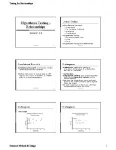
Figures 5 and 6 plot the actual values obtained for the the confidence intervals of the Time and Score variables with respect to the the equivalence intervals ∆20% and ∆50% . Computations and plots have been obtained with R scripts (R Core Team, 2012; Chen and Peace, 2011; Pikounis et al, 2001). In Figure 5 the three CIs of the Score are completely outside the equivalence intervals, so that the hypothesis of inequivalence cannot be rejected, i.e., SEF and SE are not exchangable within those ∆. In Figure 6 the three CIs are crossing the equivalence interval ∆20% but they are inside the equivalence interval ∆50% . We may conclude that whilst the methods SEF and SE are inequivalent at the level ∆20% they are equivalent at a level ∆50% . This is an interesting result derived from the EHT analysis since NHST gave the impression of the difference of the methods, but EHT establishes some level of similarity. Table 4 summarizes all results of the EHT performed on the three original crossover designs and, after comparing all CIs, we can assert that we cannot reject the null hypothesis H0 in EHT at a level of ∆20% , therefore the methods SEF and SE are inequivalent, besides being different. Widening the confidence level from 80% to 90% make the intervals larger, because of the properties of CIs, and the direct result is the inequivalence in all cases. However, we observe the equivalence of the methods in the Time variable at ∆50% . Statistically speaking, when using EHT we cannot conclude that the treatment SEF is better than the reference SE because that is not the purpose of an equivalence trial. However, by using the descriptive nature of the CIs and the previous results in NHST (Dolado et al, 2003) we observe that side-effects are harmful in all circumstances examined for the Score variable. The situation is less clear in the Time variable since equivalence can be established at the 50% level but not at the 20%. The values obtained in the confidence intervals provide a valuable information for planning future experiments, such as in the identification of critical points in understanding programs with side-effects. Bioequivalence testing helps us to take a final decision about the effects of a treatment, in our case the consequences of programming with side effects.

16

Jos´ e Javier Dolado et al.

( 5.21 , 8.29 )

|

Trial 2

( 5.7 , 8.96 )

|

Trial 1X

| |

( 7.96 , 9.71 )

|

Trial 1

− ∆20%

∆20%

0 µT − µR

|

∆50%

11

More Score in SEF

Fig. 5 Computed 80% Shortest Confidence Intervals over the Equivalence intervals ∆ in the Score variable of the Program Comprehension experiment. The three intervals are inequivalent at both ∆ levels.

( −104.62 , −34.53 )

Trial 2 |

|

( −98.48 , −40.57 )

Trial 1X

|

|

( −119.22 , −70.45 )

Trial 1

|

|

− ∆50%

− ∆20%

∆20%

0 µT − µR

Less Time in SEF

Fig. 6 Computed 80% Shortest Confidence Intervals over the Equivalence intervals ∆ in the Time variable of the Program Comprehension experiment. The three intervals are equivalent within ∆50% but not at ∆20% . Table 4 Summary of EHT on Score and Time for each Trial. Trial 1 Time

Trial 1X and Trial 2 Score

Time

Score

Confidence Level

90%

80%

90%

80%

90%

80%

90%

80%

Statistically Different? Equivalent at ∆=20%? Equivalent at ∆=50%?

Yes No Yes

Yes No Yes

Yes No No

Yes No No

Yes No Yes

Yes No Yes

Yes No No

Yes No No

6.1 Meta-analysis of the Equivalence Data In order to apply in a homogeneous way the procedures, the data of Trial 2 has to be scaled such that the results of Time and Score can be compared to those of

Equivalence Hypothesis Testing in Experimental Software Engineering

17

Trial 1 and Trial 1X. For the variable Score the transformation simply takes the range of the possible correct answers 0-14 of Trial 2 into the range 0-21 of Trial 1. For the variable Time, since there were no minimum and maximum values for the time spent in answering the questions, the transformation uses range-scaling 2 using the maximum and minimum values observed in both trials. The final CIs obtained are (−93.90, −63.81) for the Time variable and (7.02, 8.39) for the Score variable. These values are not much different from those obtained under classic meta-analysis in NHST that are (−109.01, −45.27) and (6.99, 9.14), respectively. These intervals summarize the global differences that can be observed between the SEF and SE methods, i.e., there is inequivalence of the Score variable at both levels but there is equivalence of the Time variable at 50%.

6.2 Sample Size Since there was no previous experimental data related to our research, the main source of problems for the sample size analysis was the lack of previous data about the effect size and the lack of data for computing the desired power. Hence, it was impossible to guess neither the effect-size (in absolute terms) nor the error variance. However, instead of proceeding by randomly suggesting a value we proceeded by using standardized values. 6.2.1 Classic approach to sample size In the classic NHST analysis some standard values for the Score variable were used, such as an approximate standard effect size and an estimated average correlation, obtaining a sample size between 15 and 18 subjects. In our a priori power analysis, we explored the relationships among the sample size (n), the effect size (Cohen’s f ), the significance level (α) and the desired power (1-β). We observed that there was a great variation in the sample size needed for obtaining significant results, ranging from a minimum of 6 subjects having both large correlation and large effect size, to a maximum of 209 in the opposite situation. After the data was collected the precise formulas of (Yue and Roach, 1998) were used, obtaining a sample size of 6 subjects for detecting a difference in Score of 2 correct answers. The same procedure was used for the variable Time. Therefore the sample size used was enough to give validity to the results of the SEF-SE comparison under NHST. 6.2.2 EHT approach to sample size Using the software program PASS (Hintze, 2000), that uses the TOST approach to equivalence analysis, we show in Figure 7 the plots of power versus sample size of Trial 1. The graphs in Figure 7 are plotted for power as the dependent variable and 2 The value of variable y scaled from range (y min , ymax ) into range (xmin , xmax ) is given by the transformation

yscaled = y

xmax − xmin xmin · ymax − xmax · ymin + . ymax − ymin ymax − ymin

18

Jos´ e Javier Dolado et al.

SCORE

TIME

Trial 1

Power vs N by D with Sw=1,97 LL=-2,18 UL=2,18 A=0,10 Equiv Test

Power vs N by D with Sw=54,73 LL=-75,29 UL=75,29 A=0,10 Equiv Test

1.0

1.0

0.9

0,50 1,00

0.4

0.2

1,50

9

11

13

15

17

0,00

0.8

D

0.6

Power

0,00

D

Power

0.8

0.7

30,00 40,00

0.6

0.5

20,00

9

11

N

13

15

17

N

Fig. 7 Power versus sample size in EHT for the two variables Score and Time.

they use as independent variables the sample size n and the true difference of the means D. In Figure 7 it can be observed that for achieving a given level of power the sample size should be larger as the value of the true difference D aproaches the value of the interval ∆. In the three trials the plots showed acceptable power respect to the actual number of subjects. Therefore, although for the current study sample sizes are sufficient for providing credibility to the results, researchers must be aware of the additional experimental resources that may be needed when using EHT.

7 Analysis of two Additional Software Engineering problems In order to show the application of EHT in the software engineering field, we have chosen two previous published studies. Both studies have the data publicly available and use a crossover design as the experimental setting with the subjects of the study. In this way we can apply homogeneously the procedures used in previous sections.

7.1 Dataset of the comparison of UML versus OML Here we analyse with the EHT perspective a previous experiment that compared the comprehension properties of the specification languages UML and OML (Otero and Dolado, 2005). The experimental design was a standard crossover and the NHST procedure gave as result the differences of the methods (in favour of OML) in both variables Score and Time. The experiment was repeated with a different set of subjects obtaining similar results. Applying EHT we obtain the plots of Figures 8 and 9 where we observe the inequivalence of the Score variable although there is equivalence of the Time variable at the 50% level over the reference mean.

Equivalence Hypothesis Testing in Experimental Software Engineering

19

( 0.96 , 1.49 )

|

| − ∆20%

( 0.69 , 1.51 )

| Repetition Experiment 1 |

Experiment 1

∆20% ∆50% 0 µT − µR More Score in OML

3

Fig. 8 Computed 80% Confidence Intervals over the Equivalence intervals ∆ in the Score variable of the Program Comprehension experiment. The two intervals are not equivalent within ∆50% and ∆20% .

( −804.24 , −497.59 )

|

| Repetition Experiment 1

( −815.1 , −569.47 )

|

− ∆50%

|

Experiment 1

− ∆20% Less Time in OML

0 µT − µR

∆20%

Fig. 9 Computed 80% Confidence Intervals over the Equivalence intervals ∆ in the Time variable of the Program Comprehension experiment. The two intervals are equivalent within ∆50% but not at ∆20% .

7.2 Dataset of the comparison of the specification methods UML-B versus B Here we review the crossover experiments performed by Razali et al. (Razali and Garratt, 2006; Razali et al, 2007b,a; Razali, 2008) for comparing the comprehension of two different software specification methods: a combination of a semiformal notation, UML-B, and a purely textual one, i.e., B. They used the “rate of scoring” as the measure for comparison, Efficiency, computed as marks per minute. This measure includes both variables Score and Time. Score measures the accuracy and Time measures the duration of the comprehension. In these experiments a model with a “higher rate of efficiency is better than otherwise since it indicates a higher accuracy with least time taken to understand the model”. In their first experiment they compared the efficiency in Comprehension tasks and in Modifications tasks using NHST. The authors state that (Razali et al, 2007a) “the results indicate with 95% confidence that a UML-B model could be

20

Jos´ e Javier Dolado et al.

up to 16% (Overall comprehension) and 50% (Comprehension for modification task) easier to understand than the corresponding B model”. Figure 10 shows the results of the application of EHT to their original data (Razali, 2008, pp. 337-338) for their first experiment, including both comprehension and modifications tasks. Equivalence at ∆50% over the reference mean has been found in the first dataset corresponding to the Comprehension tasks. However, the Modifications tasks show inequivalence at both levels. As replication of the first experiment, in a second crossover experiment they compared UML-B and and Event-B model and they measured also the Efficiency obtained by the subjects in six questions. Since our purpose is to assess the value of applying EHT we do not try to discuss the general conclusions of their research and methods (that included bootstraping and permutations) but to apply EHT to their basic NHST results. In this way we stick to their original data (Razali, 2008, pp. 370-371) and we proceed to analyse the six questions that were asked in their second experimental design. Their results are described in (Razali, 2008, pp.179-184) and we summarize in Table 7.2 the results stated in Table 5.6 of (Razali, 2008, p.189). It can be compared with Figure 10 and we can observe the information that EHT additionally provides to the statistical analysis. Questions 1, 3 and 6 were classified as “statistically significant” at α = 0.05 and Questions 2, 4 and 5 were assessed as “statistically not significant” with NHST. Through the application of EHT we observe that the three questions that were classified as different by NHST are identified as “inequivalent” by EHT. The other three questions that didn’t reveal differences are not equivalent at the 20% level, but Questions 2 and 5 are within a level of equivalence of 50%. Question 4 does not show any level of equivalence. We may conclude that in the first set of three questions EHT corroborates the differences originally found by NHST. Further research could be done about the equivalence found in Questions 2 and 5 and whether that has any implications in the context of their research.

Table 5 Summary of the original results of Razali et al.’s Experiment 2 (Razali, 2008, p.189) of the application of NHST to the comparison of models UML-B with Event-B.

Question Question Question Question Question Question

1 2 3 4 5 6

Mean of difference (x2) 0.8877 0.0835 0.9137 0.0487 0.0706 0.6589

Statistically Significant Yes, p=0.001 No, p=0.335 Yes, p=0.005 No, p=0.483 No, p=0.339 Yes, p=0.02

8 Related Work Besides the intensive use of bioequivalence in pharmacology, there are applications of equivalence in many other fields like psychology, ecology, plant pathology, industrial control, etc. (Cribbie et al, 2004) (Robinson and Froese, 2004) (Miranda et al, 2009) (Garrett, 1997) (Ngatia et al, 2010). Recently, there has been an application

Equivalence Hypothesis Testing in Experimental Software Engineering

|

Exp2 Q6

( 0.02 , 0.58 )

( −0.14 , 0.18 )

Exp2 Q5 Exp2 Q4 |

21

|

|

|

( −0.43 , 0.54 )

| ( 0.14 , 0.79 )

|

Exp2 Q3

|

( −0.09 , 0.18 )

|

Exp2 Q2

|

( 0.25 , 0.61 )

|

Exp2 Q1

( 0.09 , 0.48 )

|

Exp1 Modifications

|

|

( 0.02 , 0.15 )

Exp1 Comprehension

−0.9

|

|

− ∆50% − ∆20% 0 ∆20%

∆50%

0.9

µT − µR Fig. 10 Computed 90% Confidence Intervals over the Equivalence intervals ∆ in the Efficiency variable of the two experiments (Exp1 and Exp2). Experiment 1 includes two tasks and Experiment 2 has six questions.

of equivalence tests in the software engineering field (Borg and Pfahl, 2011) where the authors used EHT for analyzing the effect of using tools in the accuracy of engineers’ traceability recovery of artifacts. Their pilot experiment used 2 groups of 4 subjects and they compared the results using both NHST and EHT. Their results were inconclusive since the confidence intervals of the variables examined greatly exceded the equivalence interval established, i.e., an absolute value of ∆ = 0.05 (see Fig. 6 of (Borg and Pfahl, 2011)). That work is another example of the use of NHST and EHT in the software field. As we noted in this paper, Equivalence testing (EHT) and difference testing (NHST) are not incompatible and can be used simultaneously (Mecklin, 2003). This has previously been done in other fields of empirical research outside software engineering. For example, as long ago as 1993, Rogers et al. presented and encouragement to social scientists to consider the combined use of EHT and NHST (Rogers et al, 1993), based on the successful application to the analysis of results from drugs trials. A recent example of the application of NHST and EHT in healthcare research can be found in the findings reported by Waldhoer et al. (Waldhoer and Heinzl, 2011). Westlake proposed a procedure for computing a bioequivalence intervals (Westlake, 1976). There have been several proposals for different types of intervals such as Shortest, Fieller, Anderson-Hauck, Locke, Mandallaz-Mau’s, and some authors

22

Jos´ e Javier Dolado et al.

suggest that confidence intervals are the most reasonable way of assessing mean treatment differences. This is supported by the results of Hoenig and Heisey about the relationship between power and p-values (Tempelman, 2004) (Rani and Pargal, 2004) (Tryon, 2001). Most works that use bioequivalence methods adopt the ‘average bioequivalence mean’ for comparing treatments. However, there are situations where the withinsubject variability of a product (such as variations of more than 30% in some parameters, as in the case of highly variable drugs) make the use of the concept of average bioequivalence less appropriate. For coping with those problems there are other proposals such as the use of Population bioequivalence, Individual bioequivalence, Scaled Individual bioequivalence, Scaled Average bioequivalence and the use of different means of groups instead of only using two groups (Van Peer, 2010) (Hyslop and Iglewicz, 2001). The classic NHST has been the subject of much debate regarding its applications, uses and misuses. It has been widely observed that NHST provides only a single decision point and little information about the phenomenon being studied. This can promote, in some research communities, an almost ‘ritualistic’ application of NHST, merely in order to satisfy referees and to pass through peer review to publication, but with little thought given to the scientific interpretation of the meaning of the results and with little impact on whether or not the research findings are actionable. The literature abound on discussions about the value of the tests under NHST (see for example (Chow, 1998) for a general discussion). Independently of the value and objections to this classic approach, the NHST is based on the assumption that the null hypothesis about the means is true, something that has been questioned in other fields of study (Tryon, 2001). It has also been observed that many experimental studies do not provide enough elements to guarantee the validity of their conclusions by some statistical criteria. (Miller et al, 1997) described a set of elements that must be taken into account when designing an experiment. From this point of view, the elements that are involved in the validation of the results are: the significance level α, the sample size n, the effect size f , and the power level (1 − β), being β the probability of commiting a Type II error. However, there have been results in other fields that are also worthy of consideration. Related to the use of the power analysis, the work of (Hoenig and Heisey, 2001) criticised the common use of the concept of statistical power, 1 − β. This work had a strong impact in the field of applied statistics since it clarified the function of power analysis and suggested a reconsideration of the use of criteria derived from power analysis to assess the results of an experiment. It has been recognized by researcher in other fields (outside software engineering) that as sample size increases it also does the probability of rejecting the null hypothesis, giving to the believe that the null hypothesis is always true under many circumstances. Using NHST, the concept of power was used wrongly to assert statistical equivalence, and the usual α was used to reject H0 (Stegner et al, 1996). It has been proven that observed power is a 1:1 function of the p-value (Hoenig and Heisey, 2001). Because of the limited usefulness of the p-values, many authors advocate the use of confidence intervals instead of the p-values.

Equivalence Hypothesis Testing in Experimental Software Engineering

23

9 Conclusion Equivalence Hypothesis Testing (EHT) offers several conceptual advantages over classic t-tests under NHST, such as to allow to test for a convenient difference of the treatments and to state a more realistic null hypothesis than that of equality. We have applied EHT to the two original experimental designs about SE and SEF programs and we have rejected the equivalence of both types of programming language syntax at a level of 20%, but the inequivalence could not be established for the Time variable at a 50% level (therefore implying equivalence). There remains the transferability of the results to other settings. The current data are only a reference point for establishing differences with future trials. In a second application of EHT for the comparison of OML and UML specifications, the inequivalence in the Score variable has been established, but the Time variable has equivalence at a level of 50%. In a third application of EHT to a crossover study that compared UML-B and B specifications the original Efficiency variable was found equivalent at 50% in one dataset and inequivalent in the other. Since the Efficiency variable includes the Time variable in the computations, future studies may take into consideration this result. In the second experiment EHT has helped to assess the previous results. Classic NHST and equivalence statistical tests are not exclusive and both approaches provide useful information about the issue under experimentation. Equivalence helps to reason about intervals of interests and it is important for future studies. We have used the “average bioequivalence” criterion with the difference of the means between groups, although the ratio of the means could also have been applied. Other bioequivalence alternatives remain as other research possibilities. The main problem when using EHT is to establish the intervals for the equivalence and the related reference values. In our case, whithout knowing previously what the standard human parameters for the answers are, it is difficult to set a specific range for the Time and Scores variables. Is it enough with 15, 8 or 2 seconds of difference in the time spent in answering questions? We may ask what the effects in the large or in a software house are of a difference in the scores of 3, 4 or 2 points. Due to lacking those reference points we have used two levels for observing equivalence (20% and 50%). A related issue is to compute the sample size for a experiment using EHT. Sample size have been observed to be larger in EHT than in NHST. These are questions that remain to study. Given the fact that in software engineering the starting conditions in experiments are already different in many designs, testing for bioequivalence may be appropriate in some settings. The most important question to ask is how much differences in the treatments we allow in order to consider them as equivalent or non-equivalent. This may be difficult to answer given that human factors pervade all software engineering activities and the empirical experiments not only should try to reject the null hypothesis of indifference, but to analyse how prevailing the Type I and II errors are and what the consequences of making them are. EHT eases the reasoning on the experiment and it allows to dismiss results non-equivalent to what the researcher is looking for. Equivalence Hypothesis Testing recently (Borg and Pfahl, 2011) made the transition from empirical studies of medical trials, where it has been a proven inferential statistical analysis technique for some time, to the software engineering

24

Jos´ e Javier Dolado et al.

domain. This paper provides further evidence for the potential use of EHT as a means of checking, statistically, whether we can infer that two populations as essentially equivalent, based on samples drawn from these populations. Equivalence Hypothesis Testing combines both aspects of statistical significance and practical relevance into one procedure, by defining the reasonable limits of acceptance of the new methods under study. The use of the confidence interval approach in EHT provides an accurate description of the results and it allows the visualization of the computed results in relation to the equivalence region. Acknowledgements The authors are grateful to the reviewers for their helpful comments.

References Borg M, Pfahl D (2011) Do better ir tools improve the accuracy of engineers traceability recovery? In: Proceedings of the International Workshop on Machine Learning Technologies in Software Engineering (MALETS ’11), pp 27–34 Chen DG, Peace KE (2011) Clinical Trial Data Analysis Using R. Chapman & Hall, Boca Raton, Florida, USA Chow SC, Liu JP (2009) Design and Analysis of Bioavailability and Bioequivalence Studies. Chapman&Hall Chow SC, Wang H (2001) On sample size calculation in bioequivalence trias. Journal of Pharmacokinetics and Pharmacodynamics 28(2):155–169 Chow SL (1998) Precis of statistical significance: rationale validity and utility (with comments and reply). Behavioral and Brain Sciences 21:169–239 Cole R, McBride G (2004) Assessing impacts of dredge spoil disposal using equivalence tests: implications of a precautionary (proof of safety) approach. Marine Ecology Progress Series 279:63–72 Cribbie RA, Gruman JA, Arpin-Cribbie CA (2004) Recommendations for applying tests of equivalence. Journal of Clinical Psychology 60(1):1–10 Dolado JJ, Harman M, Otero MC, Hu L (2003) An empirical investigation of the influence of a type of side effects on program comprehension. IEEE Transactions on Software Engineering, 29(7):665–670 EMA (2010) Guideline on the investigation of bioequivalence. Tech. Rep. CPMP/EWP/QWP/1401/98 Rev. 1, EMA, European Medicines Agency Ennis D, Ennis J (2010) Equivalence hypothesis testing. Food Quality and Preference 21:253–256 Ennis DM, Ennis JM (2009) Hypothesis testing for equivalence defined on symmetric open intervals. Communications in Statistics - Theory and Methods 38(11):1792–1803 Garrett KA (1997) Use of statistical tests of equivalence (bioequivalence tests) in plant pathology. Phytopathology 87(4):372–374 Harman M (2010) Why source code analysis and manipulation will always be important. In: 10th IEEE International Working Conference on Source Code Analysis and Manipulation, Timisoara, Romania, pp 7–19 Harman M, Hu L, Zhang X, Munro M (2001) Side-effect removal transformation. In: IEEE International Workshop on Program Comprehension (IWPC 2001), Toronto, Canada, pp 309–319.

Equivalence Hypothesis Testing in Experimental Software Engineering

25

Harman M, Hu L, Hierons R, Munro M, Zhang X, Dolado J, Otero M, Wegener J (2002) A post-placement side-effect removal algorithm. In: IEEE Proceedings of the International Conference on Software Maintenance (ICSM 2002), pp 2–11 Hauschke D, Steinijans V, Pigeot I (2007) Bioequivalence Studies in Drug Development. Methods and Applications. John Wiley & Sons Hintze J (2000) PASS 2000. NCSS, LLC. Kaysville, Utah, USA Hoenig J, Heisey D (2001) The abuse of power: the pervasive fallacy of power calculations for data analysis. The American Statistician 55(1):19–24 Hyslop T, Iglewicz B (2001) Alternative cross-over designs for individual bioequivalence. In: Proceedings of the Annual Meeting of the American Statistical Association Lakhotia K, McMinn P, Harman M (2009) Automated test data generation for coverage: Haven’t we solved this problem yet? In: 4th Testing Academia and Industry Conference — Practice And Research Techniques (TAIC PART’09), Windsor, UK, pp 95–104 McBride GB (2005) Using Statistical Methods for Water Quality Management. Issues, Problems and Solutions. John Wiley & Sons Mecklin C (2003) A comparison of equivalence testing in combination with hypothesis testing and effect sizes. Journal of Modern Applied Statistical Methods 2(2):329–340 Meyners M (2012) Equivalence tests – a review. Food Quality and Preference 26(2):231–245 Miller J, Daly J, Wood M, Roper M, Brooks A (1997) Statistical power and its subcomponents – missing and misunderstood concepts in empirical software engineering research. Information and Software Technology 39(4):285–295 Miranda B, Sturtevant B, Yang J, Gustafson E (2009) Comparing fire spread algorithms using equivalence testing and neutral landscape models. Landscape Ecology 24:587–598 Ngatia M, Gonzalez D, Julian SS, Conner A (2010) Equivalence versus classical statistical tests in water quality assessments. Journal of Environmental Monitoring 12:172–177 Ogungbenro K, Aarons L (2008) How many subjects are necessary for population pharmacokinetic experiments? confidence interval approach. European Journal of Clinical Pharmacology 64:705–713 Otero MC, Dolado JJ (2005) An empirical comparison of the dynamic modeling in oml and uml. Journal of Systems and Software 77(2):91 – 102 Piaggio G, Pinol APY (2001) Use of the equivalence approach in reproductive health clinical trials. Statistics in Medicine 20(23):3571–3578 Piaggio G, Elbourne DR, Altman DG, Pocock SJ, Evans SJW (2006) Reporting of noninferiority and equivalence randomized trials. an extension of the consort statement. The Journal of the American Medical Association 295(10):1152–1160 Pikounis B, Bradstreet TE, Millard SP (2001) Graphical insight and data analysis for the 2,2,2, crossover design. In: Millard SP, Krause A (eds) Applied Statistics in the Pharmaceutical Industry with case studies using S-Plus, Springer-Verlag, pp 153–188 R Core Team (2012) R: A Language and Environment for Statistical Computing. R Foundation for Statistical Computing, Vienna, Austria Rani S, Pargal A (2004) Bioequivalence: An overview of statistical concepts. Indian Journal of Pharmacology 36(4):209–216

26

Jos´ e Javier Dolado et al.

Razali R (2008) Usability of semi-formal and formal methods integration empirical assessments. PhD thesis, School of Electronics and Computer Science, Faculty of Engineering, Science and Mathematics, University of Southampton Razali R, Garratt PW (2006) Measuring the comprehensibility of a uml-b model and a b model. In: International Conference on Computer and Information Science and Engineering (CISE 2006), pp 338–343 Razali R, Snook CF, Poppleton MR (2007a) Comprehensibility of uml-based formal model: a series of controlled experiments. In: Proceedings of the 1st ACM international workshop on Empirical assessment of software engineering languages and technologies: held in conjunction with the 22nd IEEE/ACM International Conference on Automated Software Engineering (ASE) 2007, ACM, New York, NY, USA, WEASELTech ’07, pp 25–30 Razali R, Snook CF, Poppleton MR, Garratt PW, Walters RJ (2007b) Experimental comparison of the comprehensibility of a uml-based formal specification versus a textual one. In: Kitchenham B, Brereton P, Turner M (eds) Proceedings of the 11th International Conference on Evaluation and Assessment in Software Engineering (EASE 07), British Computer Society, pp 1–11 Robinson AP, Froese RE (2004) Model validation using equivalence tests. Ecological Modelling 176(3-4):349–358 Robinson AP, Duursma RA, Marshall JD (2005) A regression-based equivalence test for model validation: shifting the burden of proof. Tree Physiology 25:903– 913 Rogers J, Howard K, Vessey J (1993) Using significance tests to evaluate equivalence between two experimental groups. Psychol Bulletin 113(3):553–565 Schuirmann DJ (1987) A comparison of the two one-sided tests procedure and the power approach for assessing the equivalence of average bioavailability. Journal of Pharmacokinetics and Biopharmaceutics 15(6):657–680 Siqueira AL, Whitehead A, Todd S, Lucini MM (2005) Comparison of sample size formulae for 2x2 cross-over designs applied to bioequivalence studies. Pharmaceutical Statistics 4:233–243 Stegner BL, Bostrom AG, Greenfield TK (1996) Equivalence testing for use in psychosocial and services research: An introduction with examples. Evaluation and Program Planning 19(3):193–198 Stein J, Doganaksoy N (1999) Sample size considerations for assessing the equivalence of two process means. Quality Engineering 12(1):105–110 Tempelman RJ (2004) Experimental design and statistical methods for classical and bioequivalence hypothesis testing with an application to dairy nutrition studies. Journal of Animal Science 82(13 suppl):E162–E172 Tryon WW (2001) Evaluating statistical difference, equivalence, and indeterminacy using inferential confidence intervals: An integrated alternative method of conducting null hypothesis statistical tests. Psychological Methods 6(4):371–386 Van Peer A (2010) Variability and impact on design of bioequivalence studies. Basic & Clinical Pharmacology & Toxicology 106(3):146–153 Waldhoer T, Heinzl H (2011) Combining difference and equivalence test results in spatial maps. International Journal of Health Geographics 10(1):3 Wellek S (2010) Testing statistical hypotheses of equivalence and noninferiority, 2nd edn. Chapman & Hall, Boca Raton, Florida, USA Westlake WJ (1976) Symmetrical confidence intervals for bioequivalence trials. Biometrics 32(4):741–744

Equivalence Hypothesis Testing in Experimental Software Engineering

27

Yue L, Roach P (1998) A note on the sample size determination in two-period repeated measurements crossover design with application to clinical trials. Journal of Biopharmaceutical Statistics 8(4):577–584