Equivariant $ K $-homology for hyperbolic reflection groups

arXiv:1707.05133v1 [math.KT] 17 Jul 2017

EQUIVARIANT K-HOMOLOGY FOR HYPERBOLIC REFLECTION GROUPS JEAN-FRANC ¸ OIS LAFONT, IVONNE J. ORTIZ, ALEXANDER RAHM, ´ J. SANCHEZ-GARC ´ ÍA AND RUBEN

Abstract. We compute the equivariant K-homology of the classifying space for proper actions, for compact 3-dimensional hyperbolic reflection groups. This coincides with the topological K-theory of the reduced C ∗ -algebra associated to the group, via the Baum-Connes conjecture. We show that, for any such reflection group, the associated K-theory groups are torsion-free. This means that previous rational computations can now be promoted to integral computations.

1. Introduction For a discrete group Γ, a general problem is to compute K∗ (Cr∗ Γ), the topological K-theory of the reduced C ∗ -algebra of Γ. The Baum-Connes Conjecture predicts that this functor can be determined, in a homological manner, from the complex representation rings of the finite subgroups of Γ. This viewpoint led to general recipes for computing the rational topological K-theory K∗ (Cr∗ Γ) ⊗ Q of groups, through the use of Chern characters (see for instance L¨ uck and Oliver [14] and L¨ uck [11], [13], as well as related earlier work of Adem [1]). When Γ has small homological dimension, one can sometimes even give completely explicit formulas for the rational topological K-theory, see for instance Lafont, Ortiz, and SánchezGarc´ıa [9] for the case where Γ is a 3-orbifold group. On the other hand, obtaining integral calculations for these K-theory groups is much harder. For 2-dimensional crystallographic groups, these were calculated in M. Yang’s thesis [22]. This was subsequently extended to the class of cocompact planar groups by L¨ uck and Stamm [16], and to certain higher dimensional dimensional crystallographic groups by Davis and L¨ uck [4] (see also Langer and L¨ uck [10]). For 3-dimensional groups, L¨ uck [12] completed this calculation for the semi-direct product Hei3 (Z) ⋊ Z4 of the 3-dimensional integral Heisenberg group with a specific action of the cyclic group Z4 . Isely [6] completed the computation for groups of the form Z2 ⋊ Z. Finally, Rahm [19] computed these for the class of Bianchi groups. In the present paper, we provide integral calculations for a further class of 3-dimensional groups. Main Theorem. Let Γ be a cocompact 3-dimensional hyperbolic reflection group, generated by reflections in the side of a hyperbolic polyhedron P ⊂ H3 . Then K0 (Cr∗ (Γ)) ≅ Zcf (Γ) and K1 (Cr∗ (Γ)) ≅ Zcf (Γ)−χ(C) , where the integers cf (Γ), χ(C) can be explicitly computed from the combinatorics of the polyhedron P. Date: July 18, 2017. 1

2

´ ÍA LAFONT, ORTIZ, RAHM, AND SANCHEZ-GARC

Let us briefly describe the contents of the paper. In Section 2, we provide background material on hyperbolic reflection groups, topological K-theory, and the Baum-Connes Conjecture. We also introduce our main tool, the Atiyah-Hirzebruch type spectral sequence. In Section 3, we use the spectral sequence to show that the K-theory groups we are interested in coincide with the Bredon homology groups Fin HFin 0 (Γ; RC ) and H1 (Γ; RC ) respectively. We also explain, using the Γ-action on 3 H , why the homology group HFin 1 (Γ; RC ) is torsion-free. In contrast, showing that Fin H0 (Γ; RC ) is torsion-free is much more difficult. We give two different arguments. In Section 4 we give a geometric argument inspired by the proof that HFin 1 (Γ; RC ) is torsion-free. This proof requires a further constraint on the vertex groups, and thus does not work in full generality. In Section 5, we give a linear algebraic proof, following the “representation ring splitting” technique of [19], which works in a broader setting. We feel it is beneficial for the reader to see both arguments, as these give very different, complementary viewpoints on the result. In addition, since these different proofs rely on different calculations, they provide (for the cases covered by both) an independent check on the result. Note that our proven lack of torsion in the Bredon homology is not a property shared by all discrete groups acting on hyperbolic 3-space: for example, 2-torsion occurs in HFin 0 (Γ; RC ) for a Bianchi group Γ whenever it has a 2-dihedral subgroup C2 × C2 [19]. Finally, in Section 6, we provide an explicit formula for the rank of the Bredon homology groups (and hence for the K-groups we are interested in), in terms of the combinatorics of the polyhedron P. Our paper concludes with three fairly long Appendices, which contain all the tables and computations used in our proofs, making our results explicit and self-contained. Acknowledgments Portions of this work were carried out during multiple collaborative visits at Ohio State University, Miami University, and the University of Southampton. The authors would like to thank these institutions for their hospitality. Lafont was partly supported by the NSF, under grant DMS-1510640. Ortiz was partly supported by the NSF, under grant DMS-1207712. Rahm was supported by Gabor Wiese’s University of Luxembourg grant AMFOR. 2. Background Material 2.1. K-theory and the Baum-Connes Conjecture. Associated to a discrete group Γ, one has Cr∗ Γ, the reduced C ∗ -algebra of Γ. This algebra is defined to be the closure, in the operator norm, of the linear span of the image of the regular representation λ ∶ Γ → B(l2 (Γ)) of Γ on the Hilbert space l2 (Γ) of square-summable complex valued functions on Γ. This algebra encodes various analytic properties of the group Γ [18]. For a C ∗ -algebra A, one can define the topological K-theory groups K∗ (A) ∶= π∗−1 (GL(A)), which are the homotopy groups of the space GL(A) of invertible matrices with entries in A. Due to Bott periodicity, there are canonical isomorphisms K∗ (A) ≅ K∗+2 (A), and thus it is sufficient to consider K0 (A) and K1 (A). In the special case where A = Cr∗ Γ, the Baum-Connes Conjecture predicts that there is a canonical isomorphism KnΓ (X) → Kn (Cr∗ (Γ)), where X is a model for EΓ (the classifying space for Γ-actions with isotropy in the family of finite subgroups), and K∗Γ (−) is the equivariant K-homology functor. The Baum-Connes conjecture

EQUIVARIANT K-HOMOLOGY FOR HYPERBOLIC REFLECTION GROUPS

3

has been verified for many classes of groups. We refer the interested reader to the monograph by Mislin and Valette [18] or the survey article by L¨ uck and Reich [15] for more information about these topics. 2.2. Hyperbolic reflection groups. By a d-dimensional hyperbolic polyhedron, we mean the region of Hd enclosed by a given finite number of (geodesic) hyperplanes, that is, the intersection of a collection of half-spaces associated to the hyperplanes. Let P ⊂ Hd be a polyhedron such that all the interior angles between faces are of the form π/mij where mij ≥ 2 an integer (although some pairs of faces may be disjoint). Let Γ = ΓP the associated Coxeter group generated by the reflections in the hyperplanes containing the faces of P. The Γ-space Hd is then a model of EΓ with fundamental domain P. This is a strict fundamental domain, that is, no further points of P are identified under the group action, and hence P = Γ/Hd (we will use left-action notation). Recall that Γ admits the following Coxeter presentation (1)

Γ = ⟨s1 , . . . , sn ∣ (si sj )mij ⟩

where n is the number of distinct hyperplanes enclosing P, si denotes the reflection on the ith face, and mij ≥ 2 are integers such that: mii = 1 for all i, and, if i ≠ j, the corresponding faces meet with interior angle π/mij . We will write mij = ∞ if the corresponding faces do not intersect. Note that P may not be a CW or simplicial complex with the natural structure given by vertices, edges, faces, etc (for example, an ideal triangle in H2 or the region enclosed by two distinct hyperplanes). However, if P has finite volume, it is a simplicial complex except from possibly ideal vertices at infinity. In such a case (i.e. P non-compact) we can obtain a cocompact model of EΓ by equivariantly removing some horoballs in Hd (see §4 in [7]). Hence a fundamental domain of the resulting action would be a copy of P with all ideal vertices truncated. For the rest of this article, d = 3, P is compact, and X is H3 with the Γ-action described above. Remark 1. We note that, by a celebrated result of Andre’ev [2], there is a simple algortithm that inputs a Coxeter group Γ, and decides whether or not there exists a hyperbolic polyhedron PΓ ⊂ H3 which generates Γ. In particular, given an arbitrary Coxeter group, one can easily verify if it is covered by the Main Theorem. 2.3. Cell structure of the orbit space. Let J = {1, . . . , n} and write ⟨S⟩ for the subgroup generated by a subset S ⊂ Γ. At a vertex of P, the concurrent faces (a minimum of 3) must generate a reflection group acting on the 2-sphere, hence it must be a spherical triangle group and in particular it forces the number of incident faces to be exactly three. The only finite Coxeter groups with 3 generators are the triangle groups ∆(2, 2, m) for some m ≥ 2, ∆(2, 3, 3), ∆(2, 3, 4) and ∆(2, 3, 5), where we use the notation (2)

∆(p, q, r) = ⟨s1 , s2 , s3 ∣ s21 , s22 , s23 , (s1 s2 )p , (s1 s3 )q , (s2 s3 )r ⟩ .

Starting from our compact polyhedron P, we obtain a Γ-CW-structure on X = H3 with: ● one orbit of 3-cells, with trivial stabilizer; ● n orbits of 2-cells (faces) with stabilisers ⟨si ⟩ ≅ Z/2 (i = 1, . . . , n);


4

● one orbit of 1-cells (edges) per (unordered) pair i, j ∈ J with mij ≠ ∞, with stabilizer ⟨si , sj ⟩ ≅ Dmij dihedral; ● one orbit of 0-cells (vertices) per (unordered) triple i, j, k ∈ J with ⟨si , sj , sk ⟩ finite, with stabilizer ⟨si , sj , sk ⟩ ≅ ∆(mij , mik , mjk ). We introduce the following notation (after having fixed an order on the Coxeter generators, or equivalently, on the faces of the polyhedron) for the simplices of P: (3)

fi

(faces),

eij

= fi ∩ fj (edges),

vijk

= fi ∩ fj ∩ fk = eij ∩ eik ∩ ejk (vertices),

whenever the intersections are non-empty, that is, whenever mij ≠ ∞, respectively when {mij , mik , mjk } equals {2, 2, m} for some m ≥ 2, {2, 3, 3}, {2, 3, 4} or {2, 3, 5}. 2.4. A spectral sequence. We ultimately want to compute the K-theory groups of the reduced C ∗ -algebra of Γ via the Baum-Connes conjecture. Note that the conjecture holds for these groups: Coxeter groups have the Haagerup property [3] and hence satisfy Baum-Connes [5]. Therefore, it suffices to compute the equivariant K-homology groups K∗Γ (X), since X is a model of EΓ. In turn, these groups can be obtained by the Bredon homology of X and an equivariant Atiyah-Hirezebruch spectral sequence coming from the inclusion of the skeleta of the Γ-CW-complex X [17]. The second page of this spectral sequence is given by the Bredon homology groups (cf. [17]) 2 Ep,q

(4)

⎧ Fin ⎪ ⎪H (Γ; RC ) =⎨ p ⎪ 0 ⎪ ⎩

q even, q odd.

The coefficients of the Bredon homology groups (a functor from the orbit category with respect to the family of finite subgroups of Γ, to Z-modules) are given by the complex representation ring of the cell stabilizers, which are finite subgroups. In order to simplify notation, we will often write Hp to denote HFin p (Γ; RC ). Before defining Bredon homology, we note that dim(X) = 3 already implies, by spectral theoretic arguments, the following. Proposition 1. There are short exact sequences 0

/ coker(d3 ) 3,0

/ K Γ (X) 0

/ H2

/0

and 0

/ H1

/ K Γ (X) 1

/ ker(d3 ) 3,0

/0.

3 3 (Here d33,0 ∶ E3,0 = H3 Ð→ E0,2 = H2 is the differential on the E 3 -page.)

Proof. This follows at once from [17, Theorem 5.29] but, for completeness, we give a direct proof based on the Atiyah-Hirzebruch spectral sequence. Write Kn for KnΓ (X). Firstly, note that the E 2 -page is concentrated in the 0 ≤ p ≤ 3 columns (since dim(X) ≤ 3), and in the q even rows —see (4) above. Secondly, recall that the bidegree of the differentials dkp,q on the E k -page is 3 (−k, k−1). Thus the only non-trivial differentials are d33,q , q ≥ 0 even, from E3,q = H3 3 3 2 ∞ 2 ∞ 3 to E0,q+2 = H0 (since E = E ). All in all, E = E except E3,q = ker(d3,q ) and


5

∞ E0,q = coker(d33,q ), that is,

∞ Ep,q

⎧ Hp p = 1, 2 and q even, ⎪ ⎪ ⎪ ⎪ ⎪ 3 ⎪ coker(d ) p = 0 and q even, ⎪ 3,0 =⎨ 3 ⎪ ker(d3,0 ) p = 3 and q even, ⎪ ⎪ ⎪ ⎪ ⎪ ⎪ otherwise. ⎩0

Now consider the filtration . . . ⊂ Fp−1,q+1 ⊂ Fp,q ⊂ . . . of Kp+q , where each Fp,q = Γ Γ Im (Kp+q (X p ) → Kp+q (X)), the image of the map induced in K-homology by the inclusion of the p-skeleton in X. In particular, Fp,q = 0 for p < 0 and Fp,q = Kp+q for ∞ 2 p ≥ dim(X) = 3. The quotient Fp,q /Fp−1,q+1 is isomorphic to Ep,q = Ep,q , as given above. Therefore we have, on one hand, the filtration: 0 = F−1,2 = F0,1 ⊂ F1,0 = F2,−1 ⊂ F3,−2 = K1 , ∞ ∞ with only two non-trivial quotients isomorphic to E1,0 = H1 and E3,−2 = ker(d33,0 ). On the other hand, we have the filtration:

0 = F−1,1 ⊂ F0,0 = F1,−1 ⊂ F2,−2 = F3,−3 = K0 , ∞ ∞ with non-trivial quotients isomorphic to E0,0 = coker(d33,0 ) and E2,−2 = H2 . These results combined together give the short exact sequences above.

2.5. Bredon Homology. To shorten notation, write Γe for stabΓ (e). The Bredon homology groups in (4) can be defined as the homology groups of the following chain complex (recall that X is a model of EΓ) (5)

/ ⊕e∈I RC (Γe ) d

...

∂d

/ ⊕e∈I RC (Γe ) d−1

/ ... ,

where Id is a set of orbit representatives of d-cells (d ≥ 0), and ∂d is defined via the geometric boundary map and induction between representation rings, as follows. If ge′ is in the boundary of e (e ∈ Id , e′ ∈ Id−1 , g ∈ Γ), then ∂ restricted to RC (Γe ) → RC (Γe′ ) is given by the composition RC (Γe )

ind

/ RC (Γge′ )

/ RC (Γe′ ) ,

≅

where the first map is the induction homomorphism of representation rings associated to the subgroup inclusion Γe ⊂ Γge′ , and the second is the isomorphism induced by conjugation Γge′ = gΓe′ g −1 . Finally, we add a sign depending on a chosen (and thereafter fixed) orientation on the faces of P. The value ∂d (e) equals the sum of these maps over all boundary cells of e. Since P is a strict fundamental domain, we can choose the faces of P as orbit representatives and thus g (as above) is always the identity. We will implicitly make this assumption from now on. 3. Analyzing the Bredon chain complex for Γ Let S = {si ∶ 1 ≤ i ≤ n} be the set of Coxeter generators and J = {1, . . . , n}. Let (6)

0

/ C3

∂3

/ C2

∂2

/ C1

∂1

/ C0

/0

be the Bredon chain complex associated to X (since X is 3-dimensional). Next we analyse each differential in the chain complex above. Recall that for a finite group G the complex representation ring RC (G) is defined as the free abelian group with basis the set of irreducible representations of G (the ring structure is


6

not relevant in this setting). Hence RC (G) ≅ Zc(G) , where we write c(G) for the set of conjugacy classes in G. 3.1. Analysis of ∂3 . Let G be a finite group with irreducible representations ρ1 , . . . , ρm of degree n1 , . . . , nm , and τ the only representation of the trivial subgroup {1G } ≤ G. Then τ induces the regular representation in G: IndG {1G } (τ ) = n1 ρ1 + . . . + nm ρm .

(7)

Lemma 1. Let X be a Γ-CW-complex with finite stabilizers, and k ∈ N. If there is a unique orbit of k-cells and this orbit has trivial stabiliser, then Hk = 0, provided that ∂k ≠ 0. Proof. The Bredon module Ck equals RC (⟨1⟩) ≅ Z with generator τ , the trivial representation. Then ∂k (τ ) ≠ 0 implies ker(∂k ) = 0 and therefore the corresponding homology group vanishes. From the lemma we immediately conclude that H3 = 0 if ∂3 ≠ 0. The case ∂3 = 0 occurs if and only if all boundary faces are pairwise identified, which cannot happen since P is a strict fundamental domain (the group acts by reflections on the faces). We conclude that H3 = 0 and, using Proposition 1, we obtain: Proposition 2. We have K1Γ (X) ≅ H1 , and there is a short exact sequence / H0

0

/ K Γ (X) 0

/ H2

/0.

3.2. Analysis of ∂2 . Let f be a face of P and e ∈ ∂f an edge. Suppose, using the notation in (3), that f = fi and e = eij . Then we have a map RC (⟨si ⟩) → RC (⟨si , sj ⟩) induced by inclusion. Recall that ⟨si ⟩ ≅ C2 and ⟨si , sj ⟩ ≅ Dmij . A straightforward analysis (see Appendix A for character tables, and Appendix B for induction homomorphism notation and calculations) shows that ̂4 + ∑ φp , ρ1 ↑ = χ1 + χ ̂3 + ∑ φp , ρ2 ↑ = χ2 + χ if i < j, or ̂3 + ∑ φp , ρ1 ↑ = χ1 + χ ̂4 + ∑ φp , ρ2 ↑ = χ2 + χ if j < i. That is, as a map of free abelian groups Z2 → Zc(Dmij ) , (a, b)

↦

(a, b)

↦

±(a, b, ̂ b, ̂ a, a + b, . . . , a + b) or ±(a, b, ̂ a, ̂ b, a + b, . . . , a + b),

Using the analysis above, we can now show Theorem 1. For any compact P, we have that H2 = 0. From this theorem and Proposition 2, we immediately obtain Corollary 1. K0Γ (X) = H0 and K1Γ (X) = H1 . Proof of Theorem. Fix an orientation on the polyhedron P, and consider the induced orientations on the faces. At an edge we have two incident faces fi and fj


7

with opposite orientations so without loss of generality we have, as a map of free abelian groups, (8)

RC (⟨si ⟩) ⊕ RC (⟨sj ⟩) ≅ Z2 ⊕ Z2

→

(a, b ∣ c, d)

↦

Zc(Dmij ) ≅ RC (⟨si , sj ⟩) (a − c, b − d, â − d, b̂ − c, S, . . . , S)

where S = a + b − c − d, and the elements with a hat ̂ appear only when mij is even. Note that we use vertical bars ‘∣’ for clarity, to separate elements coming from different representation rings. By the preceding analysis, ∂2 (x) = 0 implies that, for each i, j ∈ J, if the faces fi and fj meet, then (1) ai = aj and bi = bj , if mij is odd, and (2) ai = aj = bi = bj , if mij is even. Suppose that f1 , . . . , fn are the faces of P. Let x = (a1 , b1 ∣ . . . ∣an , bn ) ∈ C2 be an element in Ker(∂2 ). Note that ∂P is connected (since P is homeomorphic to D3 ), so by (1) and (2) above, we have that a1 = . . . = an and b1 = . . . = bn . Since the stabilizer of a vertex is a spherical triangle group, there is an even mij , which also forces a = b. Therefore we have x = (a, a∣ . . . ∣a, a) so x = ∂3 (a) (note that the choice of orientation above forces all signs to be positive), and this gives ker(∂2 ) ⊆ im(∂3 ), which suffices to prove equality and hence the vanishing of the second homology group. 3.3. Analysis of ∂1 . Let e = eij be an edge and v = vijk ∈ ∂e a vertex, using the notation in (3). We study all possible induction homomorphisms RC (⟨si , sj ⟩) → RC (⟨si , sj , sk ⟩) in Appendix B and conclude that H1 is torsion-free, as follows. Theorem 2. There is no torsion in H1 . Proof. Consider the Bredon chain complex C2

∂2

/ C1

∂1

/ C0 .

To prove that H1 = ker(∂1 )/im(∂2 ) is torsion-free, it suffices to prove that C1 /im(∂2 ) is torsion-free. Let α ∈ C1 and 0 ≠ k ∈ Z such that kα ∈ im(∂2 ). We shall prove that α ∈ im(∂2 ). Since kα ∈ im(∂2 ), we can find β ∈ C2 with ∂2 (β) = kα. Suppose that P has n faces, and write β = (a1 , b1 ∣ . . . ∣an , bn ) ∈ C2 , using vertical bars ‘∣’ to separate elements coming from different representation rings. We shall see that one can find a 1-chain β ′ , homologous to β, and with every entry of β ′ a multiple of k. At an edge eij , the differential ∂2 takes the form (cf. §3.2) (9)

RC (⟨si ⟩) ⊕ RC (⟨sj ⟩) (a, b ∣ a′ , b′ )

Ð→ RC (⟨si , sj ⟩) ↦ ±(a − a′ , b − b′ , b̂ − a′ , â − b′ ∣ S, . . . , S),

where S = a + b − a′ − b′ , and the elements with a hat ̂ appearing only when mij is even. Since every entry of ∂2 (β) is a multiple of k, using (9), we have that for every pair of intersecting faces fi and fj , ai ≡ aj (mod k)

and bi ≡ bj (mod k).

Equation (9) also shows that 1∂P = (1, 1∣ . . . ∣1, 1), the formal sum over all generators of representation rings of face stabilizers of ∂P ∈ C2 , is in the kernel of ∂2 . In particular, setting β ′ = β − a1 1∂P , we see that ∂2 (β ′ ) = ∂2 (β) = α and we can assume without loss of generality that β ′ satisfies a′1 ≡ 0 (mod k).

8


Let us consider the coefficients for the 1-chain β ′ . For every face fj intersecting f1 , we have a′1 − a′j ≡ 0 (mod k), which implies a′j ≡ 0 (mod k). Since ∂P is connected, repeating this argument we have a′i ≡ 0 (mod k) for all i. In addition, there are even mij (the stabilizer of a vertex is a spherical triangle group), and hence (9) also gives a′i − b′j ≡ 0 (mod k), which implies b′j ≡ 0 (mod k). Exactly the same argument as above gives then b′i ≡ 0 (mod k) for all i. Since all coefficients of β ′ are divisible by k, we conclude that α = ∂2 (β ′ /k) ∈ im(∂2 ), as desired. We note that a similar method of proof can be used (in many cases) to show that H0 is torsion-free. This approach is carried out in Section 4. Corollary 2. Let cf (Γ) be the number of conjugacy classes of elements of finite order in Γ, and χ(C) the Euler characteristic of the Bredon chain complex (6). Then we have H1 ≅ Zcf (Γ)−χ(C) . Proof. The Euler characteristic of a chain complex coincides with the alternating sum of the ranks of the homology groups χ(C) = rank(H0 ) − rank(H1 ) + rank(H2 ) − rank(H3 ). Since H3 = H2 = 0, we have rank(H1 ) = rank(H0 ) − χ(C), and rank(H0 ) = cf (Γ) [17]. Since H1 is torsion-free (Theorem 2), the result follows. Note that both cf (Γ) and χ(C) can be obtained directly from the geometry of the polyhedron P or, equivalently, from the Coxeter integers mij . We show this explicitly in Section 6. Remark 2. Our results agree with a previous article by three of the authors [9], where we computed the rank of the Bredon homology for groups Γ with a cocompact, 3-manifold model X of the classifying space EΓ. Firstly, note that Proposition 1 coincides with [9, Lemma 3], and, with respect to the vanishing of H3 , Proposition 2 follows from [9, Lemma 7]. The rank of H2 (X) is given in [9, Corollary 14] by β2 (Y ) if X/Γ is a closed oriented 3-manifold, or s + t′ + 2t + β2 (Y ) − 1 otherwise. Here Y is the union of the closures of all interior faces of X/Γ along with all the non-dihedral boundary components, s is the number of orientable non-odd dihedral components, t the number of orientable odd dihedral components (see [9] for definitions), t′ is the number of orientable, odd, connected components in ∂Y , and β2 () indicates the second Betti number. In our case, X/G = P has a unique boundary component, which must be dihedral (all edges stabilizers are of the form Dmij with mij ≥ 2), and there are no interior faces. Therefore Y = ∅, t′ = 0 and either s = 0 and t = 1 (if all mij are odd), or s = 0 and t = 1 (if there is at least one mij even). Picking any vertex v on ∂P , it has stabilizer which is a finite triangle group, and hence at least one mij equals 2. Thus we have indeed s = 0 and t = 1 and we conclude that rank(H2 ) = 0, as expected. The rank of H0 coincides with the number of conjugacy classes of elements of finite order in Γ. This number can be deduced from the 1-skeleton of a model of EΓ, as explained in [9, §3.2], or in §6.1 below. Finally, the rank of H1 is obtained, in both [9] and this article, from the rank of the other homology groups, and the Euler characteristic of the chain complex (5) (or (1) in [9]), which equals the alternating sum of the number of conjugacy classes in the stabilizers of Γ-orbits of cells.


9

To complete the computation of the Bredon homology, and hence of the equivariant K-homology, all that remains is the compute the torsion subgroup of H0 . We will show that in fact H0 is also torsion-free. Theorem 3. There is no torsion in H0 . An immediate consequence of Theorem 3 is Corollary 3. K0Γ (X) is torsion-free of rank cf (Γ). The arguments for Theorem 3 are quite involved. It is tempting to try to mimic the proof of Theorem 2. This approach works to some extent, as we show in Section 4 below. The arguments exploit the geometry of the polyhedron P, and rely on local analysis of the induction homomorphisms (Appendix C). Although the strategy is similar to the proof of Theorem 2, the calculations are much more involved, and only cover the case where all vertex stabilizers of P are of the form ∆(2, 2, m) with m ≥ 3 (which may vary from vertex to vertex). In order to deal with the general case, we give a second proof in Section 5 based on the representation ring splitting technique of [19]. This relies on a simultaneous basis transformation, shown in Appendix B, of the vertex blocks of ∂1 (Definition 1). This approach provides a criterion for HFin 0 (Γ; RC ) to be torsion-free which is quite efficient to check (by brute force linear algebra), and which is satisfied for Γ a hyperbolic Coxeter group. This proof, however, does not provide any particular insight into the geometry of hyperbolic Coxeter groups. In Section 6, we will give a formula for cf (Γ) and χ(C) from the geometry of the polyhedron. Combining Corollary 1, Corollary 2, and Corollary 3 immediately yields the Main Theorem. 4. No torsion in H0 – the geometric approach We present a geometric proof, similar to the proof of Theorem 2, but with further technical difficulties. The proof works under the assumption that all vertices have stabilizers of the form ∆(2, 2, m). It is not obvious how to adapt this strategy for the remaining cases, as we will explain after the proof (Remark 3). Specifically, we establish Theorem 4. Assume the compact polyhedron P is such that all vertex stabilizers are of the form Dm × Z2 , where m ≥ 3 can vary from vertex to vertex. Then there is no torsion in the 0-dimensional Bredon homology group HFin 0 (Γ; RC ). First we discuss some terminology and the overall strategy of the proof. Fix k ≥ 2 an integer. Our overall objective is to rule out k-torsion in H0 . Let β ∈ C1 (from the Bredon chain complex of Γ) such that ∂1 (β) is the zero vector modulo k. (An element α ∈ C0 has order k in H0 = C0 /im(∂1 ) if and only if kα = ∂1 (β)). Recall that C1 = ⊕ RC (⟨si , sj ⟩) , eij edge

the direct sum of the representation rings (as abelian groups) of the edge stabilisers. The element x along a particular edge eij is by definition the projection of x to Znij ≅ RC (⟨si , sj ⟩), where nij is the dimension of the representation ring (number of conjugacy classes of the edge stabiliser). By fixing β along edge eij we mean substituting β by a homologous element β ′ ∈ C1 , that is, ∂1 (β) = ∂1 (β ′ ), such that

10


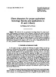
β ′ along that edge is congruent to the zero vector modulo k. When the 1-chain β is clear from the context, we will simply say that an edge e is good if all the coefficients in the chain β which are supported on e are multiples of k. We sometimes refer to an edge with stabiliser Dn as an n-edge, or edge of type n. Our goal is to replace β with a homologous chain β ′ for which all the edges are good, that is, (1) ∂1 (β ′ ) = ∂1 (β), and (2) every coefficient in the 1-chain β ′ is divisible by k. If we can do this, it follows that α = ∂1 (β ′ /k), and hence that α is zero in H0 . The construction of β ′ is elementary, but somewhat involved. It proceeds via a series of steps, which will be described in the following subsections. 4.1. Coloring the 1-skeleton. Recall that β ∈ C1 = ⊕e∈P (1) RC (Γe ), so we can view β as a formal sum of complex representations of the stabilizers of the various edges in the 1-skeleton of P. The edge stabilizers are dihedral groups. Let us 2-color the edges of the polyhedron, blue if the stabilizer is D2 , and red if the stabilizer is Dm where m ≥ 3. From our constraints on the vertex groups, we see that every vertex has exactly two incident blue edges. Of course, any graph with all vertices of degree two decomposes as a disjoint union of cycles. The collection of blue edges thus form a graph, consisting of pairwise disjoint loops, separating the boundary of the polyhedron P (topologically a 2-sphere) into a finite collection of regions, at least two of which must be contractible. The red edges appear in the interior of these individual regions, joining pairs of vertices on the boundary of the region. Fixing one such contractible region R∞ , the complement will be planar. We will henceforth fix a planar embedding of this complement. This allows us to view all the remaining regions as lying in the plane R2 .

R1

R2

R4

R3 R5

Figure 1. Example of enumeration of regions (Section 4.2). 4.2. Enumerating the regions. Our strategy for modifying β is as follows: we will work region by region. At each stage, we will modify β by only changing it on edges contained in the closure of a region. In order to do this, we need to enumerate the regions. We have already identified the (contractible) region R∞ – this will be the last region dealt with. In order to decide the order in which we will deal with the remaining regions, we define a partial ordering on the set of regions. For distinct


11

regions R, R′ , we write R < R′ if and only if R is contained in a bounded component of R2 ∖ R′ . This defines a partial ordering on the finite set of regions. For example, any region which is minimal with respect to this ordering must be simply connected (hence contractible). We can thus enumerate the regions R1 , R2 , . . . so that, for any i < j, we have Rj i, and all the remaining edges in B connect to a vj for some j < i. By the inductive hypothesis, this tells us that all but one of these red edges have coefficients congruent to (0, 0, zˆj , −ˆ zj , 0, . . . , 0) for some zj (which might depend on the edge). Again, viewing γi as a path starting and terminating at the same vertex w (where e is incident to γ), we may apply Lemma 6 and conclude that γi has coefficients along all edges that are congruent to each other. Applying Lemma 7 at the vertex w, shows that the coefficients along the


15

edge e must also be of the form (0, 0, zˆ, −ˆ z , 0, . . . , 0) for some z. This completes the inductive step and the proof of the Proposition. 4.7. Equivalence classes of red edges. Now consider a potentially bad red edge, corresponding to an edge in the graph B joining vertices vi to vj . The red edge thus joins the blue loop γi to the blue loop γj . From Proposition 3, we see that the coefficient along the red edge must be congruent to (0, 0, zˆ, −ˆ z , 0, . . . , 0) for some z. In particular, there is a single residue class that determines the coefficients along the red edge (modulo k). Next let us momentarily focus on a fixed blue loop γ, and assume the coefficients along the edges of γ are all congruent to (a, b, c, d) modulo k, as ensured by Proposition 3 (Figure 5). We define an equivalence relation on all the red edges with even label incident to γ, by defining the two equivalence classes: (a) the incident red edges that lie in the bounded region corresponding to γ, and (b) those that lie in the unbounded region. It follows from Lemma 6 (Appendix C), that all edges in the equivalence class (a) have corresponding coefficients congruent to (0, 0, zˆj , −ˆ zj , 0, . . . , 0) where each zj ≡ b − a, while all edges in equivalence class (b) have corresponding coefficients congruent to (0, 0, zˆj , −ˆ zj , 0, . . . , 0) where each zj ≡ c − a (Figure 5).

γ

zj ≡ b − a

congruent to (a, b, c, d)

zj ≡ c − a

Figure 5. Bad red edges incident to blue loop γ. All interior edges have coefficients satisfying one congruence, while all exterior edges have coefficients satisfying a different congruence (Section 4.7). This equivalence relation is defined locally, and can be extended over all blue loops/paths in the 1-skeleton, resulting in an equivalence relation on the collection of all red edges with even label. Observe that, by construction, each equivalence class has the property that there is a single corresponding residue class z mod k, with the property that all the edges within that equivalence class have coefficient congruent to (0, 0, zˆ, −ˆ z , 0, . . . , 0), i.e. the z is the same for the entire equivalence class. Corollary 4. The edges in the graph B that are bad form a finite collection of equivalence classes for this relation.

16


Proof. Let e be an edge in B, and assume that e is equivalent to an edge e′ which is not an edge in B. Since all edges that are not in B are good, it follows that the coefficient on e′ is congruent to zero mod k. Thus the value of z for the equivalence class E containing e′ is z = 0. Since e ∈ E, this forces e to be good, a contradiction. 4.8. Fixing the remaining red edges. Observe that the edges in each equivalence class form a connected subgraph, and hence a subtree (see Lemma 2), of the graph B. This collection of subtrees partitions the graph B. Any vertex of B corresponding to a blue loop is incident to at most two such subtrees (the incident red edges lying “inside” and “outside” the blue loop). On the other hand, any vertex of B corresponding to a blue path has all incident edges lying in the same subtree. We now proceed to fix our chain along the remaining red edges. Fix an equivalence class E of red edges, and associate to it a 1-chain αE whose coefficients are given as follows: (1) if a blue loop γ has an incident red edge e ∈ E, and e lies in the bounded region of γ, then assign (0, 1, 0, 0) to each blue edge on γ; (2) if a blue loop γ has an incident red edge e ∈ E, and e lies in the unbounded region of γ, then assign (0, 0, 1, 0) to each blue edge on γ; (3) along the red edges in the equivalence class (recall that all these edges have even labels), assign ±(0, 0, ˆ1, −ˆ1, 0, . . . , 0), with sign chosen to ensure that the local 1-cycle condition holds at both endpoints (see Lemma 6). Notice that, one can choose the signs in (3) coherently because the equivalence class defines a subtree of the tree B – and thus there are no cycles (these could have potentially forced the sign along an edge to be both positive and negative). Another key feature of the 1-chains αE is that they are linearly independent. More precisely, two distinct equivalence classes E, E ′ have associated 1-chains αE and αE ′ whose supports are disjoint, except possibly along a single blue loop γ. In the case where the supports overlap along γ, adding multiples of αE does not affect the z-value along the class E ′ (and vice versa). It is now immediate from the equality case of Lemma 6 in Appendix C that the 1-chain αE is in fact an integral 1-cycle. Subtracting multiples of αE from our given chain β, we may thus obtain a homologous 1-chain for which all the red edges in E are now good. Repeating this for each of the equivalence classes, we have now obtained a homologous 1-chain (still denoted β) for which all the red edges are good. 4.9. Fixing the remaining blue edges. We now have obtained a 1-chain with prescribed differential, whose coefficients along all red edges are good. It remains to fix the coefficients along the blue loops. If γ is one of the blue loops, then since all incident red edges are good, we see that all the edges on γ have coefficients which are congruent to either (a, b, c, d), (a, b, a, b), (a, a, c, c), or (a, a, a, a), according to the equivalence classes that are incident to γ. Let us discuss, as an example, the case (a, b, a, b). Note that this case occurs if the only incident red edges to γ with even label lie in the unbounded region determined by γ. Consider the pair of integral 1-cycles α13 , α24 supported on γ, obtained by assigning to each edge on γ the coefficient (1, 0, 1, 0) and (0, 1, 0, 1) respectively. From the equality case of Lemma 6 we see that α13 , α24 are in fact 1-cycles. By adding multiples of α13 , α24 , we can now arrange for the coefficients


17

along the blue loop γ to all be good. The three other cases can be dealt with similarly; we leave the details to the reader. 4.10. Completing the proof. Performing this process described in Section 4.9 for all the blue components, we finally obtain the desired 1-chain β ′ . Since β ′ now satisfies properties (1) and (2) mentioned at the beginning of the proof, we conclude that the given hypothetical torsion class α ∈ H0 was in fact the zero class. This completes the proof of Theorem 4. Remark 3. It is not obvious how to adapt the strategy in the geometric proof above to the case when other vertex stabilizer types are allowed. In the case of vertex stabilizers of the type ∆(2, 3, 3), ∆(2, 3, 4), and ∆(2, 3, 5), most of the arguments can be adapted. The main difficulty lies in the arguments of Subsection 4.4, which rely heavily on Lemma 6 in Appendix C. Unfortunately, the analogue of that Lemma does not seem to hold when one allows these other types of vertices as endpoints of the edge. For vertices with stabilizer ∆(2, 2, 2), additionally difficulties arise, notably in Sections 4.7, 4.8, and 4.9. 5. No torsion in H0 – the linear algebra approach In this section we prove that H0 is torsion-free for all vertex types. We will describe the general strategy, leaving the explicit calculations (simultaneous base transformations, and corresponding induction homomorphisms) for Appendices A and B. This proof follows the “representation ring splitting” technique of [19]. We start with a simple linear algebra lemma. Lemma 3. For square matrices M and B, we have M det ( ∗

0 ) = det(M ) ⋅ det(B). B

Proof. Writing M = (ai,j ) and denoting by M i,j the (i, j)-minor of M (that is, the determinant of the block obtained by omitting the i-th row and the j-th column), we have #M M 0 det ( ) = ∑ a1,j (−1)1+j M 1,j ⋅ det(B), ∗ B j=1 by iterating the development of the determinant by minors (#M − 1) times, and making use of the zero block each time. Definition 1. The vertex block of a given vertex v in a Bredon chain complex differential matrix ∂1 consists of all the blocks of ∂1 that are representing maps induced (on complex representation rings from Γe → Γv ) by edges e adjacent to v. Therefore, if v is adjacent to edges e1 , e2 and e3 , with corresponding representation rings of rank n1 , n2 and n3 , then its vertex block is a submatrix of δ1 (identified with its matrix representation after fixing a basis) of size n1 + n2 + n3 by n0 , the rank of RC (Γv ). Our strategy is based on the following criterion that guarantees that HFin 0 (Γ; RC ) is torsion-free. Theorem 5. If there exists a base transformation such that all minors in all vertex blocks are in the set {−1, 0, 1}, then HFin 0 (Γ; RC ) is torsion-free.

18


Proof. As a generality on Smith Normal Forms, known already to Smith [21], we note that the elementary divisors of a matrix A can be computed (up to multiplicai (A) tion by a unit) as αi = ddi−1 , where di (A) (called i-th determinant divisor) equals (A) the greatest common divisor of all i × i minors of the matrix A, and d0 (A) ∶= 1. Let us use the notation pre-rank(∂1 ) ∶= rankZ C1 − rankZ ker ∂1 , where C1 is the module of 1-chains in the Bredon chain complex. Then HFin 0 (Γ; RC ) is torsion-free if and only if αi = ±1 for all 1 ≤ i ≤ pre-rank(∂1 ), which, by the remark above, follows from finding an (i × i)-minor in the Bredon chain complex differential matrix ∂1 with value ±1, for each 1 ≤ i ≤ pre-rank(∂1 ). Let us show this is indeed the case, by induction on i. Induction basis. For i = 1, we observe that there are vertices with adjacent edges for the action of Γ, hence there are non-zero vertex blocks. As by assumption all the entries in the vertex blocks are in the set {−1, 0, 1}, there exists an entry of value ±1. Inductive step. Let 2 ≤ i ≤ pre-rank(∂1 ), and assume that there exists an (i − 1) × (i − 1)-minor of ∂1 of value ±1. We have to find an i × i-minor of ∂1 of value ±1. Let B ′ be the (i − 1) × (i − 1)-block of ∂1 , whose determinant is ±1 according to the inductive hypothesis. As i ≤ pre-rank(∂1 ), there exists a vertex block V with the following property : After suitable base transformation, which puts V into the upper left corner of ∂1 , the block B ′ can be extended to an i × i-block B ′′ = det (

M ∗

0 ), B

with B a square sub-block of B ′ , and M a square sub-block of V . Here, B is completely disjoint with V , and therefore we get the zero block in the upper right corner of B ′′ (note that the vertex blocks have been constructed to contain all entries from adjacent edges, so the remainders of their rows are zero). In case that B ′ is already disjoint with V , we simply have B = B ′ , and M is then a single entry of V . Otherwise, we construct B as the maximal square sub-block of B ′ that has all of its rows and columns outside rows and columns in which V is present. Then M is constructed by taking the intersection of B ′ and V , and extending it to a square block of size n − size(B) inside V . Lemma 3 yields det(B ′′ ) = det(M ) ⋅ det(B). Now det(M ) ∈ {−1, 0, 1} by the assumption that there is no torsion in the vertex blocks; and as n ≤ pre-rank(∂1 ), we can reach det(B ′′ ) ≠ 0 and hence det(M ) ≠ 0. For B as a sub-block of B ′ , det(B ′ ) ∈ {−1, 1} entails det(B) ∈ {−1, 1}. This implies det(B ′′ ) = ±1 and we are done. Using Theorem 5, the lack of non-trivial torsion in H0 is a consequence of the following result, whose proof depends on the simultaneous base transformations in Appendix B. Proposition 4. For a system of finite subgroups of types A5 × C2 , S4 , S4 × C2 , ∆(2, 2, 2) = (C2 )3 and ∆(2, 2, m) = C2 × Dm for m ≥ 3 as vertex stabilizers, with their three 2-generator Coxeter subgroups as adjacent edge stabilizers, there is a simultaneous base transformation such that all vertex blocks have all their minors contained in the set {−1, 0, 1}.


19

Proof. We apply the base transformation specified in Appendix B (all Tables referenced in this proof can be found there). Then we already see that all of the induced maps have all of their entries in the set {−1, 0, 1}. Next, we assemble the vertex blocks from the three vertex-edge-adjacency induced maps for any given vertex stabilizer type. By Tables 24 and 25, the vertex block of a stabilizer of type Dm for m ≥ 3 odd consists of

two blocks

⎛1 ⎜0 ⎜ ⎜0 ⎜ ⎜⋮ ⎜ ⎜ ⎜0 ±⎜ ⎜0 ⎜ ⎜ ⎜0 ⎜ ⎜0 ⎜ ⎜ ⎜⋮ ⎝0

0 0 0 ⋮ 0 1 0 0 ⋮ 0

0⎞ 1⎟ ⎟ 0⎟ ⎟ ⋮⎟ ⎟ ⎟ 0⎟ ⎟ 0⎟ ⎟ ⎟ 0⎟ ⎟ 0⎟ ⎟ ⎟ ⋮⎟ 0⎠

0 0 0 ⋮ 0 0 1 0 ⋮ 0

identity matrix of size 0

and one block ± (

m+3 2 ).

By Lemma 3, the columns which are concentrated in one entry ±1 cannot increase the absolute value of the determinant of a block which is being extended into them. We conclude that all minors are in {0, ±1}. For m ≥ 6 even, but not a power of 2, Tables 26 and 27 yield the following vertex block, where each matrix block is specified up to orientation sign (we make this assumption from now on), Dm × C2 ρ 1 ⊗ χ1 ↓ ρ1 ⊗ (χ2 − χ1 ) ↓ ρ1 ⊗ (χ3 − χ2 ) ↓ ρ1 ⊗ (χ4 − χ1 ) ↓ ρ1 ⊗ (φ1 − χ3 − χ1 ) ↓ ⋮ ρ1 ⊗ (φp − φp−1 ) ↓ ⋮ ρ1 ⊗ (φ m −1 − φ m −2 ) ↓ 2 2 (ρ2 − ρ1 ) ⊗ χ1 ↓ (ρ2 − ρ1 ) ⊗ (χ2 − χ1 ) ↓ (ρ2 − ρ1 ) ⊗ (χ3 − χ2 ) ↓ (ρ2 − ρ1 ) ⊗ (χ4 + χ3 − χ2 − χ1 ) ↓ (ρ2 − ρ1 ) ⊗ (φ1 − χ2 − χ1 ) ↓ ⋮ ρ1 ⊗ (φp − φp−1 ) ↓ ⋮ ρ1 ⊗ (φ m −1 − φ m −2 ) ↓ 2

1 0 0 0 0 0 0

0 1 0 0 0 0 0

Dm ↪ Dm × C2 0 0 0 0 0 1 0 0 1 −1 0 0 0 1 0 0 0 1 1 0 0 0 0 ⋱ 0 0 0 0

0 0 0 0 0 0 1

0

2

D2 1 0 0 0 0 ⋮ 0 0 0 0 0 0 ⋮ 0

↪ D m × C2 0 0 0 0 0 1 0 0 0 0 0 0 0 0 0 ⋮ ⋮ ⋮ 0 0 0 1 0 0 0 1 0 0 0 0 0 0 0 0 0 0 ⋮ ⋮ ⋮ 0 0 0

D2 1 0 0 0 0 ⋮ 0 0 0 0 0 0 ⋮ 0

↪ Dm × C2 0 0 0 0 0 1 0 0 0 0 0 0 0 0 0 ⋮ ⋮ ⋮ 0 0 0 1 0 0 0 1 0 0 0 0 0 0 0 0 0 0 ⋮ ⋮ ⋮ 0 0 0

By Lemma 3, we can ignore the rows and columns which have at most one entry ±1, and reduce the above vertex block to the finite block ⎛ ⎜ ⎜ ⎜ ⎝

1 0 0 0

0 1 0 0

1 −1 1 1

0 0 0 1

±1 0 0 0

±1 0 0 0

⎞ ⎟ ⎟, ⎟ ⎠

for which we can easily check that it has all its minors in {0, ±1}.


20

For m ≥ 4 a power of 2, Tables 28 and 29 yield the following vertex block, Dm × C2 ρ 1 ⊗ χ1 ↓ ρ1 ⊗ (χ2 − χ1 ) ↓ ρ1 ⊗ (χ3 − χ1 ) ↓ ρ1 ⊗ (χ4 − χ2 ) ↓ ρ1 ⊗ (φ1 − χ2 − χ1 ) ↓ ⋮ ρ1 ⊗ (φp − φp−1 ) ↓ ⋮ (φ m −1 − φ m −2 ) ↓ 2 2 (ρ2 − ρ1 ) ⊗ χ1 ↓ (ρ2 − ρ1 ) ⊗ (χ2 − χ1 ) ↓ (ρ2 − ρ1 ) ⊗ (χ3 − χ1 ) ↓ (ρ2 − ρ1 ) ⊗ (χ4 + χ3 − χ2 − χ1 ) ↓ (ρ2 − ρ1 ) ⊗ (φ1 − χ2 − χ1 ) ↓ ⋮ ρ1 ⊗ (φp − φp−1 ) ↓ ⋮ ρ1 ⊗ (φ m −1 − φ m −2 ) ↓ 2

Dm ↪ Dm × C2 0 0 0 0 0 1 0 1 0 0 1 1 0 0 0 −1 0 0 0 0 0 1 0 1 0 0 0 0 0 ⋱ 0 0 0 0 0

1 0 0 0 0 0 0

0 0 0 0 0 0 1

0

2

D2 1 0 0 0 0 ⋮ 0 0 0 0 0 0 ⋮ 0

↪ Dm × C2 0 0 0 0 0 1 0 0 0 0 0 0 0 0 0 ⋮ ⋮ ⋮ 0 0 0 1 0 0 0 1 0 0 0 0 0 0 0 0 0 0 ⋮ ⋮ ⋮ 0 0 0

D2 1 0 0 0 0 ⋮ 0 0 0 0 0 0 ⋮ 0

↪ Dm × C2 0 0 0 0 0 1 0 0 0 0 0 0 0 0 0 ⋮ ⋮ ⋮ 0 0 0 1 0 0 0 1 0 0 0 0 0 0 0 0 0 0 ⋮ ⋮ ⋮ 0 0 0

By Lemma 3, we can ignore the rows and columns which have at most one entry ±1, and reduce the above vertex block to the finite block ⎛ ⎜ ⎜ ⎜ ⎜ ⎜ ⎜ ⎝

1 0 0 0 0

0 1 1 −1 0

0 0 1 0 1

0 1 0 0 0

0 0 0 0 1

±1 0 0 0 0

0 ±1 0 0 0

±1 0 0 0 0

0 ±1 0 0 0

⎞ ⎟ ⎟ ⎟, ⎟ ⎟ ⎟ ⎠

for which we can easily check that it has all its minors in {0, ±1}. For the finitely many remaining stabilizer types, we can proceed case-by-case: we input each vertex block into a computer routine which computes all of its minors (such a routine is straightforward to implement and takes approximately two seconds per vertex block on a standard computer; the third author’s implementation is available at http://math.uni.lu/˜rahm/vertexBlocks/). Note that for the groups under consideration, the matrix rank of the vertex block is at most 7, so the 8 × 8-minors are all zero, and it is enough to compute the n × n-minors for n ≤ 7. Corollary 5. For any Coxeter group Γ having a system of finite subgroups of types ∆(2, 2, 2) = (C2 )3 , ∆(2, 2, m) = C2 × Dm for m ≥ 3, S4 , S4 × C2 or A5 × C2 as vertex stabilizers, we have that the Bredon homology group HFin 0 (Γ; RC ) is torsion-free. Remark 4. Note that to use the criterion in Theorem 5 for proving that HFin n (Γ; RC ) is torsion-free for a group Γ, the following should be taken into account: (a) The proof of the theorem, stated for n = 0, implicitly uses the fact that H0 (BΓ; Z) is always torsion-free. To extend the theorem to n > 0, one should either work with groups for which Hn (BΓ; Z) is torsion-free (such as Coxeter groups), or use the splitting described in section 7 of [19] in order to make a statement only about the part of HFin n (Γ; RC ) complementary to Hn (BΓ; Z). (b) Before trying to prove the hypothesis in the theorem using base transformations (as in Appendix A), which can become quite laborious, one should construct the vertex blocks without any base transformation and compute their elementary divisors. If there exists a suitable simultaneous base transformation which proves the criterion, then those elementary divisors must be in the set {−1, 0, 1}. Hence if that is not the case, no simultaneous base transformation can exist.


21

6. cf (Γ) and χ(C) from the geometry of P Let Γ be the reflection group of the compact 3-dimensional hyperbolic polyhedron P. In this section, we compute the number of conjugacy classes of elements of finite order of Γ, cf (Γ), and the Euler characteristic of the Bredon chain complex (5), χ(C), from the geometry of the polyhedron P. This makes our Bredon homology, and equivariant K-theory results, in particular the Main Theorem, explicit. 6.1. Conjugacy classes of elements of finite order. We now give an algorithm to calculate cf (Γ), the number of conjugacy classes of elements of finite order in the Coxeter group Γ. We know that each element of finite order can be conjugated to one which stabilizes one of the k-dimensional faces of the polyhedron, for some k ∈ {0, 1, 2}. Of course, the only element which stabilizes all faces is the identity element. Let us set that aside, and consider the non-identity elements, to which we associate the integer k. We now count the elements according to the integer k, in descending order. Case k = 2: These are the conjugacy classes represented by the canonical generators of the Coxeter group Γ. The number of these is given by the total number ∣P (2) ∣ of facets of the polyhedron P. Case k = 1: These elements are edge stabilizers which are not conjugate to the stabilizer of a face. We first note that there are some possible conjugacies between edge stabilizers. Geometrically, these occur when there is a geodesic γ ⊂ H3 whose projection onto the fundamental domain P covers multiple edges inside the 1-skeleton P (1) . A detailed analysis of when this can happen is given in [8]. Following the description in that paper, we decompose the 1-skeleton into equivalence classes of edges, where two edges are equivalent if there exists a geodesic whose projection passes through both edges. Denote by [P (1) ] the set of equivalence classes of edges, and note that each equivalence class [e] has a well defined group associated to it, which is just the dihedral group Γe stabilizing a representative edge. We can thus count the conjugacy classes in the corresponding dihedral group, and discard the three conjugacy classes already accounted for (the conjugacy class of the two canonical generators counted in case k = 2, as well as the identity). Thus the contribution from finite elements of this type is given by ∑

(c(Γe ) − 3).

[e]∈[P (1) ]

(Recall that c(Dm ), the number of conjugacy classes in a dihedral group of order 2m, is m/2 + 3 if m even, and (m − 1)/2 + 2 if m is odd.) Case k = 0: Finally, we consider the contribution from the elements in the vertex stabilizers which have not already been counted. That is to say, for each vertex v ∈ P (0) , we count the conjugacy classes of elements in the corresponding 3-generated spherical triangle group, which cannot be conjugated into one of the canonical 2generated special subgroups. This number, c¯(Γv ), depends only on the isomorphism type of the spherical triangle group Γv , see Table 1. The contribution from these types of finite elements is thus ∑ c¯(Γv ) .

v∈P (0)


22

Γv ∆(2, 2, m) ∆(2, 3, 3) ∆(2, 3, 4) ∆(2, 3, 5)

c(Γv ) 2 c(Dm ) 5 10 10

c¯(Γv ) c(Dm ) − 3 1 3 5

Table 1. Number of conjugacy classes in spherical triangle groups. The left column is the total number (cf. Appendix A), and the right column the number of those not conjugated into one of the three canonical 2-generated special subgroups.

Combining all these, we obtain the desired (combinatorial) formula for the number of conjugacy classes of elements of finite order inside the group Γ: cf (Γ) = 1 + ∣P (2) ∣ +

∑

(c(Γe ) − 3) + ∑ c¯(Γv ) .

[e]∈[P (1) ]

v∈P (0)

6.2. Euler characteristic. The Euler characteristic of the Bredon chain complex can be easily calculated from the stabilizers of the various faces of the polyhedron P, according to the formula: χ(C) = ∑ (−1)dim(f ) dim(RC (Γf )) . f ∈P

Depending on the dimension of the faces, we know exactly what the dimension of the complex representation ring is (the number of conjugacy classes in the stabilizer): ● for the 3-dimensional face (the interior), the stabilizer is trivial, so there is a 1-dimensional complex representation ring; ● for the 2-dimensional faces, the stabilizer are Z2 , and there is a 2-dimensional complex representation ring; ● for the 1-dimensional faces e, the stabilizers are dihedral groups, and there is a c(Γe )-dimensional complex representation ring; ● for the 0-dimensional faces v, the stabilizers are spherical triangle groups, and there is a c(Γv )-dimensional complex representation ring. Putting these together, we obtain χ(C) = −1 + 2∣P (2) ∣ − ∑ c(Γe ) + ∑ c(Γv ) . e∈P (1)

v∈P (0)

All in all, we have a more explicit version of the Main Theorem, from the geometry of the polyhedron P. Main Theorem (explicit). Let Γ be a cocompact 3-dimensional hyperbolic reflection group, generated by reflections in the side of a hyperbolic polyhedron P ⊂ H3 . Then K0 (Cr∗ (Γ)) is a torsion-free abelian group of rank cf (Γ) = 1 + ∣P (2) ∣ + and

K1 (Cr∗ (Γ))

∑

(c(Γe ) − 3) + ∑ c¯(Γv ) ,

[e]∈[P (1) ]

v∈P (0)

is a torsion-free abelian group of rank

cf (Γ) − χ(C) = 2 − ∣P (2) ∣ +

∑

(c(Γe ) − 3) + ∑ c(Γe ) − ∑ (c(Γv ) − c¯(Γv )) ,

[e]∈[P (1) ]

e∈P (1)

v∈P (0)

and the values c(Γv ) and c¯(Γv ) can be obtained from Table 1.


23

References [1] A. Adem. Characters and K-theory of discrete groups. Invent. Math., 114(3):489–514, 1993. [2] E. M. Andreev. Convex polyhedra of finite volume in Lobaˇ cevski˘ı space. Mat. Sb. (N.S.), 83 (125):256–260, 1970. [3] M. Bo˙zejko, T. Januszkiewicz, and R. J. Spatzier. Infinite Coxeter groups do not have Kazhdan’s property. J. Operator Theory, 19(1):63–67, 1988. [4] J. F. Davis and W. L¨ uck. The topological K-theory of certain crystallographic groups. J. Noncommut. Geom., 7(2):373–431, 2013. [5] N. Higson and G. Kasparov. Operator K-theory for groups which act properly and isometrically on Hilbert space. Electron. Res. Announc. Amer. Math. Soc., 3:131–142 (electronic), 1997. [6] O. Isely. K-theory and K-homology for semi-direct products of Z2 by Z. 2011. Th` ese de doctorat : Universit´ e de Neuchˆ atel (Switzerland). [7] J.-F. Lafont, B. A. Magurn, and I. J. Ortiz. Lower algebraic K-theory of certain reflection groups. Math. Proc. Cambridge Philos. Soc., 148(2):193–226, 2010. [8] J.-F. Lafont and I. J. Ortiz. Lower algebraic K-theory of hyperbolic 3-simplex reflection groups. Comment. Math. Helv., 84(2):297–337, 2009. [9] J.-F. Lafont, I. J. Ortiz, and R. J. S´ anchez-Garc´ıa. Rational equivariant K-homology of low dimensional groups. In Topics in noncommutative geometry, volume 16 of Clay Math. Proc., pages 131–163. Amer. Math. Soc., Providence, RI, 2012. [10] M. Langer and W. L¨ uck. Topological K-theory of the group C ∗ -algebra of a semi-direct product Zn ⋊ Z/m for a free conjugation action. J. Topol. Anal., 4(2):121–172, 2012. [11] W. L¨ uck. Chern characters for proper equivariant homology theories and applications to Kand L-theory. J. Reine Angew. Math., 543:193–234, 2002. [12] W. L¨ uck. K- and L-theory of the semi-direct product of the discrete 3-dimensional Heisenberg group by Z/4. Geom. Topol., 9:1639–1676, 2005. [13] W. L¨ uck. Rational computations of the topological K-theory of classifying spaces of discrete groups. J. Reine Angew. Math., 611:163–187, 2007. [14] W. L¨ uck and B. Oliver. Chern characters for the equivariant K-theory of proper G-CWcomplexes. In Cohomological methods in homotopy theory (Bellaterra, 1998), volume 196 of Progr. Math., pages 217–247. Birkh¨ auser, Basel, 2001. [15] W. L¨ uck and H. Reich. The Baum-Connes and the Farrell-Jones conjectures in K- and Ltheory. In Handbook of K-theory. Vol. 1, 2, pages 703–842. Springer, Berlin, 2005. [16] W. L¨ uck and R. Stamm. Computations of K- and L-theory of cocompact planar groups. K-Theory, 21(3):249–292, 2000. [17] G. Mislin. Equivariant K-homology of the classifying space for proper actions. In Proper group actions and the Baum-Connes conjecture, Adv. Courses Math. CRM Barcelona, pages 1–78. Birkh¨ auser, Basel, 2003. [18] G. Mislin and A. Valette. Proper group actions and the Baum-Connes conjecture. Advanced Courses in Mathematics. CRM Barcelona. Birkh¨ auser Verlag, Basel, 2003. [19] A. D. Rahm. Sur la K-homologie ´ equivariante de PSL2 sur les entiers quadratiques imaginaires. Ann. Inst. Fourier, 66(4):1667–1689, 2016. [20] J.-P. Serre. Linear representations of finite groups. Springer-Verlag, New York-Heidelberg, 1977. Translated from the second French edition by Leonard L. Scott, Graduate Texts in Mathematics, Vol. 42. [21] H. J. S. Smith. On systems of linear indeterminate equations and congruences. Philosophical transactions of the Royal Society of London, 151:293–326, 1861. [22] M. Yang. Crossed products by finite groups acting on low dimensional complexes and applications. ProQuest LLC, Ann Arbor, MI, 1997. Thesis (Ph.D.)–The University of Saskatchewan (Canada).

24


Appendix A. Character tables and base transformations In this Appendix, we list the character tables of all the groups involved in the Bredon chain complex (6), that is, finite Coxeter subgroups of Γ up to rank three. This serves as a reference for the main text, and fixes the notation. In the character tables below, rows correspond to irreducible representations, and columns to representatives of conjugacy classes, written in term of the Coxeter generators s1 , . . . , sn in a fixed Coxeter presentation of Γ, as in (1). In addition, for each character table, we apply elementary row operations to obtain the transformed tables needed for Appendix B, which are in turn used in the linear algebra proof that H0 is torsion-free (Section 5). Although the rows of the transformed tables do no more consist of irreducible characters, it is easy to check that they still constitute bases of the complex representation rings. Note that, for consistency across subgroups, we will pay attention to the order of the Coxeter generators in a subgroup. We write e for the identity element in Γ. A.1. Rank 0. This is the trivial group, with character table given below.

τ

e 1

Table 2. Character table of the trivial group.

A.2. Rank 1. A rank 1 Coxeter group is a cyclic group of order 2. Write si for its Coxeter generator, then its character table is Table 3 below. C2 ρ1 ρ2

e si 1 1 1 −1

Table 3. Character table of ⟨si ⟩ ≅ C2 .

A.3. Rank 2. A finite rank 2 Coxeter group with Coxeter generators si and sj is a dihedral group of order m = mij ≥ 2, (10)

Dm = ⟨si , sj ∣ s2i = s2j = (si sj )m ⟩ .

The character table of this group is given in Table 4 below, where 0 ≤ r ≤ m − 1, p varies between 1 and m/2 − 1 if m is even or (m − 1)/2 if m is odd, and the hat ̂ denotes a character which appear only when m is even. In order to be consistent, we assume the Coxeter generators are ordered so that i < j. If j < i, then the character table is identical except that the third and fourth rows (the characters ̂3 and χ ̂4 ) are interchanged, since (sj si )r = (si sj )−r and si (sj si )r = sj (si sj )−r−1 . χ For the case m = 2, that is, D2 = C2 × C2 , we will sometimes use the notation coming from the character table of C2 (Table 3) instead. (Recall that the irreducible characters of a direct product G × H are obtained from the irreducible characters of G and H as ρi ⊗τj , where (ρi ⊗ τj ) (g, h) = ρi (g)⋅τj (h).) This gives the notation and


Dm χ1 χ2 ̂3 χ ̂4 χ φp

25

(si sj )r sj (si sj )r 1 1 1 −1 (−1)r (−1)r r (−1) (−1)r+1 2πpr 2 cos ( m ) 0

Table 4. Character table of < si , sj >≅ Dm , where i < j.

characters in Table 5, which are equivalent to Table 4 with ρ1 ⊗ρ1 = χ1 , ρ1 ⊗ρ2 = χ4 , ρ2 ⊗ ρ1 = χ3 and ρ2 ⊗ ρ2 = χ2 . As before, we assume i < j, or, if j < i, the third and fourth rows (characters) must be interchanged. C2 × C2 ρ1 ⊗ ρ1 ρ1 ⊗ ρ2 ρ2 ⊗ ρ1 ρ2 ⊗ ρ2

e si sj si sj 1 1 1 1 1 1 −1 −1 1 −1 1 −1 1 −1 −1 1

Table 5. Alternative character table of ⟨si , sj ⟩ ≅ D2 = C2 × C2 , i < j.

We now give the base transformations of the character table of Dm needed later, shown in Tables 6, 7 and 8. D2 ∑ χi χ2 + χ3 χ3 χ3 + χ4

e si sj 4 0 2 0 1 −1 2 −2

si 0 −2 −1 0

sj 0 0 1 0

Table 6. Base transformation of the character table of D2 .

A.4. Rank 3. A finite rank 3 Coxeter subgroup is one of the spherical triangle groups ∆(2, 2, m), with m ≥ 2, ∆(2, 3, 3), ∆(2, 3, 4), or ∆(2, 3, 5), using the notation in (2), or, more compactly, the Coxeter diagrams in Figure 6. m

4

5

Figure 6. Coxeter diagrams of rank 3 spherical Coxeter groups. In these diagrams, the vertices represent Coxeter generators and the edges are labelled by mij , with the conventions: no edge if mij = 2, and no label if mij = 3.


26

si

si sj

(si sj )r

χ1 + χ2 + 2 ∑p=1 φp

2m

0

0

⋯

0

χ2 + ∑p=1 φp

m

−1

0

⋯

0

∑p=1 φp

m−1

0

−1

⋯

−1

m − 2k + 1 2

⋮ 0

ak,1 b1

ak,r br

ak, m−1 2 b m−1 2

m−1 2

m−1 2

m−1 2

⋮

m−1 2

∑p=k φp φ m−1 2

⋮

(si sj )

m−1 2

e

Dm

Table 7. Base transformation of the character table of Dm , m ≥ 3 m−1 2 ), br ∶= 2 cos( π(m−1)r ), and 1 < 2 cos( 2πpr odd. Here, ak,r ∶= ∑p=k m m k, r < m−1 . 2

Dm m 4 2 −1 φp ∑p=1 χp + 2 ∑p=1 m 2 −1 χ2 + χ3 + ∑p=1 φp m 2 −1 χ3 + ∑p=1 φp m 2 −1 χ2 + χ4 + ∑p=1 φp m 2 −1 φp ∑p=1 m 2 −1 ⋮ ∑p=k φp ⋮ φ m2 −1

e 2m m m−1 m m−2 m − 2k 2

si 0 0 1 −2 0 ⋮ 0

si sj 0 0 −1 0 0 ak,1 b1

(si sj )r ⋯ ⋯ ⋯ ⋯ −1 − (−1)r ak,r br

m

(si sj ) 2 0 0 −1 0 m −1 − (−1) 2 m 2 −1 2 ∑p=k (−1)p m 2(−1) 2 −1

sj si sj 0 −2 −1 0 0 0 0

Table 8. Base transformation of the character table of Dm , m ≥ 4 m 2 −1 even. Here, ak,r ∶= ∑p=k 2 cos( 2πpr ), br ∶= 2 cos( π(m−2)r ), 1 < k < m m m m − 1 and 1 < r < . 2 2

A.4.1. ∆(2, 2, 2). This triangle group is isomorphic to C2 × C2 × C2 and we have irreducible characters ρabc ∶= ρa ⊗ρb ⊗ρc , a, b, c ∈ {1, 2}, from Table 3, listed in Table 9 below, where ρa ⊗ ρb ⊗ ρc (x) = ρa (x1 ) ⋅ ρb (x2 ) ⋅ ρc (x3 ) for all x = (x1 , x2 , x3 ) ∈ C2 × C2 × C2 . Here we assume that we have ordered the Coxeter generators si , sj , sk so that i < j < k. Finally, the base transformation of the character table of ∆(2, 2, 2) needed later is shown in Table 10. A.4.2. ∆(2, 2, m) with m > 2. This group is isomorphic to C2 ×Dm , and has Coxeter presentation ∆(2, 2, m) = ⟨si , sj , sk ∣ s2i , s2j , s2k , (si sj )2 , (si sk )2 , (sj sk )m ⟩ , where we have sorted the Coxeter generators sj and sk such that j < k (the generator si is uniquely determined from the presentation). As a direct product of two groups, the character table of this group can be obtained from those of C2 (Table 3) and Dm (Table 4). This is shown on Table 11, where TDm is the matrix of entries of the character table of Dm (Table 4). As explained before, if k < j one needs to swap the characters χ3 and χ4 , that is, swap ρ1 ⊗ χ3 and ρ1 ⊗ χ4 , and ρ2 ⊗ χ3 and ρ2 ⊗ χ4 .


C2 × C2 × C2 ρ111 ∶= ρ1 ⊗ ρ1 ⊗ ρ1 ρ112 ∶= ρ1 ⊗ ρ1 ⊗ ρ2 ρ121 ∶= ρ1 ⊗ ρ2 ⊗ ρ1 ρ122 ∶= ρ1 ⊗ ρ2 ⊗ ρ2 ρ211 ∶= ρ2 ⊗ ρ1 ⊗ ρ1 ρ212 ∶= ρ2 ⊗ ρ1 ⊗ ρ2 ρ221 ∶= ρ2 ⊗ ρ2 ⊗ ρ1 ρ222 ∶= ρ2 ⊗ ρ2 ⊗ ρ2

e 1 1 1 1 1 1 1 1

si 1 1 1 1 −1 −1 −1 −1

sj 1 1 −1 −1 1 1 −1 −1

27

sk si sj si sk sj sk si sj sk 1 1 1 1 1 −1 1 −1 −1 −1 1 −1 1 −1 −1 −1 −1 −1 1 1 1 −1 −1 1 −1 −1 −1 1 −1 1 1 1 −1 −1 1 −1 1 1 1 −1

Table 9. Character table of ⟨si , sj , sk ⟩ ≅ ∆(2, 2, 2) = C2 × C2 × C2 , i < j < k, from Table 3.

C2 × C2 × C2 ρ111 ρ112 − ρ111 ρ121 − ρ111 ρ122 − ρ121 ρ211 − ρ111 ρ212 − ρ211 ρ221 − ρ121 ρ222 − ρ221

e si sj 1 1 1 0 0 0 0 0 −2 0 0 0 0 −2 0 0 0 0 0 −2 0 0 0 0

sk si sj si sk sj sk si sj sk 1 1 1 1 1 −2 0 −2 −2 −2 0 −2 0 −2 −2 −2 0 −2 2 2 0 −2 −2 0 −2 −2 0 2 −2 2 0 2 −2 0 2 −2 0 2 2 −2

Table 10. Base transformation of the character table of ⟨si , sj , sk ⟩ ≅ ∆(2, 2, 2) = C2 × C2 × C2 , i < j < k.

∆(2, 2, m) ρ1 ⊗ χ1 ρ1 ⊗ χ2 ̂3 ρ1 ⊗ χ ̂4 ρ1 ⊗ χ ρ1 ⊗ φ p ρ2 ⊗ χ1 ρ2 ⊗ χ2 ̂3 ρ2 ⊗ χ ̂4 ρ2 ⊗ χ ρ2 ⊗ φ p

(sj sk )r

sk (sj sk )r

si (sj sk )r

si sk (sj sk )r

TDm

TDm

TDm

−TDm

Table 11. Character table of ∆(2, 2, m), m = mjk > 2, j < k.

The corresponding base transformations for ∆(2, 2, m) ≅ C2 × Dm are given in Table 12 (m odd), Table 13 (m ≥ 6 even not a power of 2), and Table 14 (m ≥ 4 a power of 2).


28

Dm × C2 ρ1 ⊗ χ 1 ρ1 ⊗ (χ2 − χ1 ) ρ1 ⊗ (φ1 − χ2 − χ1 ) ρ1 ⊗ (φp − φp−1 ), (ρ2 − ρ1 ) ⊗ χ1 (ρ2 − ρ1 ) ⊗ (χ2 − χ1 ) (ρ2 − ρ1 ) ⊗ (φ1 − χ2 − χ1 ) (ρ2 − ρ1 ) ⊗ (φp − φp−1 ),

e 1 0 0 0 0 0 0 0

si 1 −2 0 0 0 0 0 0

(si sj )r 1 0 br ap,r 1 0 0 0

α 1 0 0 0 −2 0 0 0

αsi 1 −2 0 0 −2 4 −4 0

α(si sj )r 1 0 br ap,r −2 0 −2br −2ap,r

Table 12. Base transformation of the character table of Dm × C2 for m ≥ 3 odd. Here ap,r ∶= 2 cos( 2πpr ) − 2 cos( 2π(p−1)r ), br ∶= m m m−1 2πr 2 cos( m ) − 2, 2 ≤ p ≤ 2 and 1 ≤ r ≤ m − 1.

Dm × C2 ρ1 ⊗ χ1 ρ1 ⊗ (χ2 − χ1 ) ρ1 ⊗ (χ3 − χ2 ) ρ1 ⊗ (χ4 − χ1 ) ρ1 ⊗ (φ1 − χ3 − χ1 ) ⋮ ρ1 ⊗ (φp − φp−1 ) ⋮ (ρ2 − ρ1 ) ⊗ χ1 (ρ2 − ρ1 ) ⊗ (χ2 − χ1 ) (ρ2 − ρ1 ) ⊗ (χ3 − χ2 ) (ρ2 − ρ1 ) ⊗ (χ4 + χ3 − χ2 − χ1 ) (ρ2 − ρ1 ) ⊗ (φ1 − χ2 − χ1 ) (ρ2 − ρ1 ) ⊗ (φp − φp−1 )

si 1 −2 2 −2 −2 0 0 0 0 0 0 0

(si sj )r 1 0 cr cr br ap,r 0 0 0 0 0 0

sj si sj 1 −2 0 0 0 0 0 0 0 0 0 0

αsi 1 −2 2 −2 −2 0 −2 4 −4 0 0 0

α(si sj )r 1 0 cr cr br ap,r −2 0 −2cr −4cr −2(br + cr ) −2ap,r

αsj si sj 1 −2 0 0 0 0 −2 4 0 0 0 0

Table 13. Base transformation of the character table of Dm × C2 for m ≥ 6 even, not a power of 2. Here ap,r ∶= 2 cos( 2πpr )− m 2π(p−1)r 2πr r r 2 cos( m ), br ∶= 2 cos( m ) − (−1) − 1, cr = (−1) − 1 and 1 < p, r < m . 2

A.4.3. ∆(2, 3, 3). This triangle group has Coxeter presentation (11)

∆(2, 3, 3) = ⟨si , sj , sk ∣ s2i , s2j , s2k , (si sj )3 , (si sk )2 , (sj sk )3 ⟩ .

This group is, in standard notation, A3 , and it is isomorphic to the symmetric group S4 , with Coxeter generators si = (1 2), sj = (2 3) and sk = (3 4), for instance. Then we have conjugacy classes (cycle types in S4 ) represented, in terms of the Coxeter generators, by si = (1 2), si sj = (1 3 2), si sj sk = (1 4 3 2) and si sk = (1 2)(3 4). In particular, we have the character table for ∆(2, 3, 3) shown in Table 15 below. In this case, the Coxeter generators are unique up to conjugation since Out(S4 ) is trivial, hence the choice of si and sk does not affect the character table. The required base transformation of the character table Table 15 is given in Table 16. A.4.4. ∆(2, 3, 4). This triangle group has Coxeter presentation (12)

∆(2, 3, 4) = ⟨si , sj , sk ∣ s2i , s2j , s2k , (si sj )3 , (si sk )2 , (sj sk )4 ⟩ ,


Dm × C2 ρ1 ⊗ χ 1 ρ1 ⊗ (χ2 − χ1 ) ρ1 ⊗ (χ3 − χ2 ) ρ1 ⊗ (χ4 − χ1 ) ρ1 ⊗ (φ1 − χ3 − χ1 ) ⋮ ρ1 ⊗ (φp − φp−1 ) ⋮ (ρ2 − ρ1 ) ⊗ χ1 (ρ2 − ρ1 ) ⊗ (χ2 − χ1 ) (ρ2 − ρ1 ) ⊗ (χ3 − χ2 ) (ρ2 − ρ1 ) ⊗ (χ4 + χ3 − χ2 − χ1 ) (ρ2 − ρ1 ) ⊗ (φ1 − χ2 − χ1 ) (ρ2 − ρ1 ) ⊗ (φp − φp−1 )

si 1 −2 0 0 0 0 0 0 0 0 0 0

(si sj )r 1 0 cr cr br ap,r 0 0 0 0 0 0

sj si sj 1 −2 −2 2 0 0 0 0 0 0 0 0

αsi 1 −2 0 0 0 0 −2 4 0 0 0 0

α(si sj )r 1 0 cr cr br ap,r −2 0 −2cr −4cr −2br −2ap,r

29

αsj si sj 1 −2 −2 2 0 0 −2 4 4 0 0 0

Table 14. Base transformation of the character table of Dm × C2 for m ≥ 4 even a power of 2. Here ap,r ∶= 2 cos( 2πpr )− m 2πr m r 2 cos( 2π(p−1)r ), b ∶= 2 cos( ) − 2, c = (−1) − 1 and 1 < p, r < . r r m m 2

∆(2, 3, 3) ξ1 ξ2 ξ3 ξ4 ξ5

e 1 1 2 3 3

si 1 −1 0 1 −1

si sj 1 1 −1 0 0

si sj sk 1 −1 0 −1 1

si sk 1 1 2 −1 −1

Table 15. Character table of ⟨si , sj , sk ⟩ ≅ ∆(2, 3, 3) ≅ S4 .

S4 ξ1 ξ̃2 ∶= ξ2 − ξ1 ξ̃3 ∶= ξ3 − ξ2 − ξ1 ξ̃4 ∶= ξ4 − ξ3 − ξ1 ̃ ξ5 ∶= ξ5 − ξ4 − ξ2 + ξ1

e 1 0 0 0 0

si 1 −2 0 0 0

si sj 1 0 −3 0 0

si sj sk 1 −2 0 −2 4

si sk 1 0 0 −4 0

Table 16. Base transformation of the character table of ∆(2, 3, 3) ≅ S4 .

and the Coxeter generators are uniquely determined from the presentation. In standard notation, this is the finite Coxeter group B3 (or C3 ). This group is isomorphic to S4 ×C2 with Coxeter generators, for instance, si = (1 2)α, sj = (1 3)α and sk = (1 2)(3 4)α, where α is the generator of the C2 factor. We can choose representatives of the conjugacy classes in terms of the Coxeter generators, for


30

example, e ∼ e

α ∼ (si sj sk )3

(1 2) ∼ si sk

(1 2)α ∼ si

(1 2 3) ∼ si sj

(1 2 3)α ∼ si sj sk

(1 2 3 4) ∼ sj sk

(1 2 3 4)α ∼ si (sj sk )2

(1 2)(3 4) ∼ (sj sk )2

(1 2)(3 4)α ∼ sk

where ‘∼’ means ‘conjugate’. Using this representatives, and the fact that ∆(2, 3, 4) is a direct product, the character table of this group can be written as in Table 17 below, where TS4 is the matrix of coefficients of the character table of S4 (Table 15). S4 × C2 ρ1 ⊗ ξ1 ρ1 ⊗ ξ2 ρ1 ⊗ ξ3 ρ1 ⊗ ξ4 ρ1 ⊗ ξ5 ρ2 ⊗ ξ1 ρ2 ⊗ ξ2 ρ2 ⊗ ξ3 ρ2 ⊗ ξ4 ρ2 ⊗ ξ5

e

si sk

si sj

sj sk

(sj sk )2

(si sj sk )3

si

si sj sk

TS4

TS4

TS4

−TS4

si (sj sk )2

sk

Table 17. Character table of ⟨si , sj , sk ⟩ ≅ ∆(2, 3, 4) = S4 × C2 .

The base transformation needed is given in Table 18, where {ξ̃i } is the transformed basis of the character table of S4 , Table 16. A.4.5. ∆(2, 3, 5). This group has Coxeter presentation (13)

∆(2, 3, 5) = ⟨si , sj , sk ∣ s2i , s2j , s2k , (si sj )3 , (si sk )2 , (sj sk )5 ⟩

and it is isomorphic to A5 × C2 with Coxeter generators si = (1 2)(3 5)α, sj = (1 2)(3 4)α, sk = (1 5)(2 3)α, for example. In standard notation, this is the exceptional finite Coxeter group H3 . Remark 5. These Coxeter generators are not unique, since Out(A5 × C2 ) ≅ C2 . There are then two sets of Coxeter generators up to conjugation, the other one given by conjugation by a suitable g ∈ S5 ∖ A5 , for instance, conjugating by g = (2 4): s′i = (1 4)(3 5)α, s′j = (1 4)(2 3)α, s′k = (1 5)(3 4)α. In the first case sj sk = (1 3 4 2 5), conjugated to (1 2 3 4 5), and in the second case s′j s′k = (1 3 2 4 5), conjugated to (1 3 2 4 5), which represent different conjugacy classes in A5 .


S4 × C2 α1 α2 α3 α4 α5 α6 α7 α8 α9 α10

(1) 1 0 0 0 0 0 0 0 0 0

(12) 1 −2 0 −2 0 2 −4 0 0 0

(123) 1 0 −3 0 0 0 0 0 0 0

(1234) 1 −2 0 4 4 2 0 0 6 0

(12)(34) 1 0 0 −4 0 0 0 0 −4 0

α 1 0 0 2 0 −2 0 0 4 0

α(12) 1 −2 0 0 0 0 0 0 0 0

α(123) 1 0 −3 2 0 −2 0 6 4 0

α(1234) 1 −2 0 6 4 0 4 0 −6 −8

31

α(12)(34) 1 0 0 −2 0 −2 0 0 8 0

where α1 ∶= ρ1 ⊗ ξ1 , α2 ∶= ρ1 ⊗ ξ̃2 , α3 ∶= ρ1 ⊗ ξ̃3 , α4 ∶= ρ1 ⊗ (ξ̃4 + 2ξ̃5 ) − (ρ2 ⊗ ξ1 − ρ1 ⊗ ξ2 ), α5 ∶= ρ1 ⊗ ξ̃5 , α6 ∶= ρ2 ⊗ ξ1 − ρ1 ⊗ ξ2 , α7 ∶= ρ2 ⊗ ξ2 − ρ2 ⊗ ξ1 + ρ1 ⊗ (ξ5 − ξ4 ), α8 ∶= (ρ2 − ρ1 ) ⊗ ξ̃3 , α9 ∶= ρ2 ⊗ (ξ̃4 + 2ξ̃5 ) + (ρ1 − ρ2 ) ⊗ (ξ1 + ξ2 ), α10 ∶= (ρ2 − ρ1 ) ⊗ ξ̃5 .

Table 18. Base transformation of the character table of ⟨si , sj , sk ⟩ ≅ ∆(2, 3, 4) = S4 × C2 .

A character table for the alternating group A5 reads as follows. A5 ξ1 ξ2 ξ3 ξ4 ξ5

e 1 4 5 3 3

(1 2 3) 1 1 −1 0 0

(1 2)(3 4) 1 0 1 −1 −1

(1 2 3 4 5) 1 −1 0√ 1+ 5 2√ 1− 5 2

(1 3 4 5 2) 1 −1 0√ 1− 5 2√ 1+ 5 2

If we call TA5 the matrix of coefficients of this table then the character table of ∆(2, 3, 5) is given by Table 19, where we have used the following representatives of the conjugacy classes in terms of the Coxeter generators (‘∼’ means ‘conjugate’) e ∼ e

α ∼ (si sj sk )5

(1 2 3) ∼ si sj

(1 2 3)α ∼ si (sj sk )2

(1 2)(3 4) ∼ si sk

(1 2)(3 4)α ∼ si

(1 2 3 4 5) ∼ sj sk

(1 2 3 4 5)α ∼ si sj sk

(1 2 3 5 4) ∼ (si sj sk )

4

(1 2 3 5 4)α ∼ sj si sk

Remark 6. With the non-conjugate set of Coxeter generators s′i , s′j , s′k (see Remark 5), we get the analogous set of representatives except swapping the obvious ones, that is, sj sk ∼ (s′i s′j s′k )4 , (si sj sk )4 ∼ s′j s′k , (si sj sk )5 sj sk ∼ s′i s′j s′k and si sj sk ∼ (s′i s′j s′k )5 s′j s′k . On the character table this amounts to interchanging ρi ⊗ ξ4 with ρi ⊗ ξ5 for i = 1 and 2.


32

A5 × C2 ρ1 ⊗ ξ1 ρ1 ⊗ ξ2 ρ1 ⊗ ξ3 ρ1 ⊗ ξ4 ρ1 ⊗ ξ5 ρ2 ⊗ ξ1 ρ2 ⊗ ξ2 ρ2 ⊗ ξ3 ρ2 ⊗ ξ4 ρ2 ⊗ ξ5

e

si sj

si sk

sj sk

(si sj sk )4

(si sj sk )5

si (sj sk )2

si

TA5

TA5

TA5

−TA5

si sj sk

sj si sk

Table 19. Character table of ⟨si , sj , sk ⟩ ≅ ∆(2, 3, 5) = A5 × C2 .

For the base transformation required, first note that the character table for the alternating group A5 above can be transformed as follows, A5 ξ1 ξ̃2 ∶= ξ2 − 4ξ1 ξ̃3 ∶= ξ3 − ξ2 − ξ1 ξ̃4 ∶= ξ4 − ξ2 + ξ1 ̃ ξ5 ∶= ξ5 + ξ4 − ξ1 − ξ3

e 1 0 0 0 0

(1 2 3) 1 −3 −3 0 0

(1 2)(3 4) 1 −4 0 0 −4

(1 2 3 4 5) 1 −5 0√

(1 3 4 5 2) 1 −5 0√

0

0

5+ 5 2

5− 5 2

and then A5 ξ1 ̃ ̃ ̃ ξ2 ∶= ξ2 − ξ̃3 − ξ̃5 ξ̃3 ξ̃4 ξ̃5

e 1

(1 2 3) 1

(1 2)(3 4) 1

(1 2 3 4 5) 1

(1 3 4 5 2) 1

0 0 0 0

0 −3 0 0

0 0 0 −4

−5 0√

−5 0√

5+ 5 2

5− 5 2

0

0

With this notation, the required base transformation is given in Table 20. Appendix B. Induction homomorphisms In this Appendix, we compute all possible induction homomorphisms RC (H) → RC (G) appearing in the Bredon chain complex (6). That is, G is a finite Coxeter subgroup of Γ of rank n generated by n ≤ 3 of the Coxeter generators (1), and H is a subgroup of G generated by a subset of exactly n − 1 of those Coxeter generators. We give explicit induction homomorphisms with respect to the standard character tables, and also with respect to the transformed bases in Appendix A for rank 3 subgroups, as this is needed for the simultaneous base transformation argument in the linear algebra proof that HFin 0 (Γ; RC ) is torsion-free (Section 5). We implicitly use the character tables and notation in Appendix A, and Frobenius reciprocity [20], throughout this Appendix. We also note that Frobenius reciprocity extends linearly:


A5 × C2 β1 β2 β3

e 1 0 0

s i sj 1 0 −3

si sk 1 0 0

β4 β5 β6 β7 β8 β9 β10

0 0 0 0 0 0 0

0 0 0 0 0 0 0

0 −4 0 0 0 0 0

sj sk √1 5 0√

5+ 5 2

0 0 0 0 0 0

(si sj sk )4 1 √ − 5 0√

(si sj sk )5 1 0 0

si (sj sk )2 1 0 −3

si 1 0 0

0 0 0 0 0 0

0 4 −2 0 0 0 −8

0 4 −2 0 6 0 −8

0 0 −2 0 0 0 0

5− 5 2

33

si sj sk √1 5 0√

sj si sk 1 √ − 5 0√

4 −2 10 0√ −5 − 5 −8

4 −2 10 0√ −5 + 5 −8

5+ 5 2

5− 5 2

̃ where β1 ∶= ρ1 ⊗ ξ1 , β2 ∶= ρ1 ⊗ ξ̃2 + 2ρ1 ⊗ ξ̃4 , β3 ∶= ρ1 ⊗ ξ̃3 , β4 ∶= ρ1 ⊗ ξ̃4 , ̃ ̃ β5 ∶= ρ1 ⊗ ξ5 − 2(ρ2 − ρ1 ) ⊗ ξ1 , β6 ∶= (ρ2 − ρ1 ) ⊗ ξ1 , β7 ∶= (ρ2 − ρ1 ) ⊗ ξ̃2 , β8 ∶= (ρ2 − ρ1 ) ⊗ ξ̃3 , β9 ∶= (ρ2 − ρ1 ) ⊗ ξ̃4 , β10 ∶= (ρ2 − ρ1 ) ⊗ (ξ̃5 + 4ξ1 ).

Table 20. Base transformation of the character table of ⟨si , sj , sk ⟩ ≅ ∆(2, 3, 5) = A5 × C2 .

Lemma 4. If H is a subgroup of a finite group G and φ and η, respectively τ and π, are representations of G, respectively H, then (φ ↓ +ξ ↓ ∣τ + π) = (φ + ξ∣τ ↑ +π ↑) . Proof. 1 ∑ (φ ↓ +ξ ↓)(h) ⋅ (τ + π)(h) ∣H∣ h∈H 1 = ∑ (φ ↓ ⋅τ + ξ ↓ ⋅τ + φ ↓ ⋅π + ξ ↓ ⋅π)(h) ∣H∣ h∈H

(φ ↓ +ξ ↓ ∣τ + π) =

which by Frobenius reciprocity on irreducible characters equals 1 ∑ (φ ⋅ τ ↑ +ξ ⋅ τ ↑ +φ ⋅ π ↑ +ξ ⋅ π ↑)(h) = (φ + ξ∣τ ↑ +π ↑) . ∣G∣ g∈G

B.1. Rank 1. The only induction homomorphism in this case is RC ({e}) → RC (⟨si ⟩) which must the regular representation τ ↦ ρ1 + ρ2 shown, in terms of free abelian groups, in Figure 7. RC ({e})

→ RC (C2 )

Z

→ Z2

a

↦ (a, a)

Figure 7. Induction homomorphism from H = {e} to G = ⟨si ⟩ ≅ C2 .


34

B.2. Rank 2. In this case G is a dihedral group with the presentation G = ⟨si , sj ∣ s2i = s2j = (si sj )m ⟩ , where m = mij and we assume i < j. Consider first the case H = ⟨si ⟩. The characters of Dm (Table 5) restricted to H are (note that si = sj (si sj )m−1 ) Dm ↓ χ1 χ2 ̂3 χ ̂4 χ φp

e si 1 1 1 −1 1 −1 1 1 2 0

Multiplying with the rows of the character table of H ≅ C2 (Table 3) we obtain the induced representations ̂4 + ∑ φp , ρ1 ↑ = χ1 + χ ̂3 + ∑ φp . ρ2 ↑ = χ2 + χ The other case is when H = ⟨sj ⟩. This is analogous, but note that, in order to keep the notation consistent with Table 4, the characters χ3 and χ4 must be interchanged in the even case. Specifically, we have now sj = sj (si sj )0 and hence Dm ↓ χ1 χ2 ̂3 χ ̂4 χ φp

e sj 1 1 1 −1 1 1 1 −1 2 0

and therefore ̂3 + ∑ φp , ρ1 ↑ = χ1 + χ ̂4 + ∑ φp . ρ2 ↑ = χ2 + χ All in all, as maps of free abelian groups, we have that the induction homomorphisms RC (H) → RC (G) shown in Figure 8. RC (H)

→

RC (G)

2

→

(a, b)

↦

Zc(Dm ) (a, b, ̂ b, ̂ a, a + b, . . . , a + b)

(a, b)

↦

Z

(a, b, ̂ a, ̂ b, a + b, . . . , a + b)

for H = ⟨si ⟩, for H = ⟨sj ⟩,

Figure 8. Induction homomorphisms from H to G = ⟨si , sj ⟩ ≅ Dm , m = mij and i < j.

B.3. Rank 3. We compute each case individually.


35

B.3.1. G = ∆(2, 2, 2). This group is isomorphic to C2 × C2 × C2 , and has Coxeter generators si , sj , sk where i < j < k. We compute the induction homomorphisms for the Coxeter subgroups ⟨si , sj ⟩, ⟨si , sk ⟩ and ⟨sj , sk ⟩, all three direct factors of G and isomorphic to C2 × C2 . Using the bases of RC (C2 × C2 ) and RC (∆(2, 2, 2)) induced from C2 (Tables 5 and 9), we immediately obtain the induction homomorphisms shown, as maps of free abelian groups, shown in Figure 9. Remark 7. Recall how to the induction homomorphism works from a group A to direct product A × B: if ρ is a representation of A then IndA×B (ρ) = ρ ⊗ rB , where A rB is the regular representation of B. RC (H)

→

RC (G)

4

→

Z8

(a, b, c, d)

↦

(a, a, b, b, c, c, d, d)

for H = ⟨si , sj ⟩,

(a, b, c, d)

↦

(a, b, a, b, c, d, c, d)

for H = ⟨si , sk ⟩,

(a, b, c, d)

↦

(a, b, c, d, a, b, c, d)

for H = ⟨sj , sk ⟩.

Z

Figure 9. Induction homomorphisms from H to G = ⟨si , sj , sk ⟩ ≅ ∆(2, 2, 2) = C2 × C2 × C2 , and i < j < k. On the other hand, with respect to the transformed bases (Tables 6 and 10 in Appendix A), the induction homomorphisms take the form shown in Tables 21, 22, and 23. Note that, for the transformed bases, we show the restricted characters, and the induced map, in two adjacent tables separated by double vertical bars. ⟨sj , sk ⟩ ↪ C2 × C2 × C2 ρ111 ↓ ρ112 − ρ111 ↓ ρ121 − ρ111 ↓ ρ122 − ρ121 ↓ ρ211 − ρ111 ↓ ρ212 − ρ211 ↓ ρ221 − ρ121 ↓ ρ222 − ρ221 ↓

e 1 0 0 0 0 0 0 0

sj 1 0 −2 0 0 0 0 0

sk 1 −2 0 −2 0 −2 0 −2

sj sk 1 −2 −2 2 0 −2 0 2

(⋅∣ ∑ χi ) 1 0 0 0 0 0 0 0

(⋅∣χ2 + χ3 ) 0 1 0 1 0 1 0 1

(⋅∣χ3 + χ4 ) 0 0 1 0 0 0 0 0

(⋅∣χ4 ) 0 0 1 −1 0 0 0 −1

Table 21. Restricted characters and induced map ⟨sj , sk ⟩ ↪ ∆(2, 2, 2) = C2 × C2 × C2 .

B.3.2. G = ∆(2, 2, m), m > 2. This group is isomorphic to C2 × Dm with Coxeter presentation ∆(2, 2, m) = ⟨si , sj , sk ∣ s2i , s2j , s2k , (si sj )2 , (si sk )2 , (sj sk )m ⟩ , We have three relevant Coxeter subgroups H, which we treat separately. In each case, we restrict the characters of G (Table 11) to the subgroup H and then use Frobenius reciprocity to write the induced characters of H into G in terms of the characters of G.

36


⟨si , sk ⟩ ↪ C2 × C2 × C2 ρ111 ↓ ρ112 − ρ111 ↓ ρ121 − ρ111 ↓ ρ122 − ρ121 ↓ ρ211 − ρ111 ↓ ρ212 − ρ211 ↓ ρ221 − ρ121 ↓ ρ222 − ρ221 ↓

(⋅∣χ2 + χ3 ) 0 1 0 1 0 1 0 1

(⋅∣χ3 + χ4 ) 0 0 0 0 1 0 1 0

Table 22. Restricted characters and induced map ∆(2, 2, 2) = C2 × C2 × C2 .

⟨si , sk ⟩ ↪

⟨si , sj ⟩ ↪ C2 × C2 × C2 ρ111 ↓ (ρ112 − ρ111 ) ↓ (ρ121 − ρ111 ) ↓ (ρ122 − ρ121 ) ↓ (ρ211 − ρ111 ) ↓ (ρ212 − ρ211 ) ↓ (ρ221 − ρ121 ) ↓ (ρ222 − ρ221 ) ↓

e 1 0 0 0 0 0 0 0

e 1 0 0 0 0 0 0 0

si 1 0 0 0 −2 0 −2 0

si 1 0 0 0 −2 0 −2 0

sk 1 −2 0 −2 0 −2 0 −2

sj 1 0 −2 0 0 0 0 0

si sk 1 −2 0 −2 −2 2 −2 2

si sj 1 0 −2 0 −2 0 2 0

(⋅∣ ∑ χi ) 1 0 0 0 0 0 0 0

(⋅∣ ∑ χi ) 1 0 0 0 0 0 0 0

(⋅∣χ2 + χ3 ) 0 0 1 0 0 0 0 0

(⋅∣χ3 + χ4 ) 0 0 0 0 1 0 1 0

(⋅∣χ4 ) 0 0 0 0 1 −1 1 −1

(⋅∣χ4 ) 0 0 0 0 1 0 0 0

Table 23. Restricted characters and induced map D2 ≅ ⟨si , sj ⟩ ↪ ∆(2, 2, 2) = C2 × C2 × C2 .

Case 1: H = ⟨si , sj ⟩ ≅ D2 = C2 × C2 . The elements e, si , sj and si sj of H are obtained from the 1st, 3rd, 2nd and 4th column of Table 11 for r equals 0, 0, n−1 and n−1 respectively, giving the restrictions (by abuse of notation we indicate the restricted character with the same symbols): C2 × Dm ↓ ρ1 ⊗ χ1 ρ1 ⊗ χ2 ̂3 ρ1 ⊗ χ ̂4 ρ1 ⊗ χ ρ1 ⊗ φp ρ2 ⊗ χ1 ρ2 ⊗ χ2 ̂3 ρ2 ⊗ χ ̂4 ρ2 ⊗ χ ρ2 ⊗ φp

e 1 1 1 1 2 1 1 1 1 2

si 1 1 1 1 2 −1 −1 −1 −1 −2

sj 1 −1 −1 1 0 1 −1 −1 1 0

si sj 1 −1 −1 1 0 −1 1 1 −1 0

Now we use Frobenius reciprocity (multiply the rows of the character tables of H with those of G ↓ H above, and divide by ∣H∣ = 4) to obtain the coefficients of the induced irreducible representations of H in G in terms of the irreducible representations of G. If i < j then the character table of H is the one given in Table 5, but if j < i we should interchange the second and third characters (rows) in that


37

table. This gives ρ1 ⊗ ρ1 ↑ ρ1 ⊗ ρ2 ↑ ρ2 ⊗ ρ1 ↑ ρ2 ⊗ ρ2 ↑

= = = =

ρ1 ⊗ χ1 + ρ̂ 1 ⊗ χ 4 + ∑ ρ1 ⊗ φp ρ1 ⊗ χ2 + ρ̂ 1 ⊗ χ 3 + ∑ ρ1 ⊗ φp ρ2 ⊗ χ1 + ρ̂ 2 ⊗ χ 4 + ∑ ρ2 ⊗ φp ρ2 ⊗ χ2 + ρ̂ 2 ⊗ χ 3 + ∑ ρ2 ⊗ φp

if i < j, and

ρ1 ⊗ ρ1 ↑ = ρ1 ⊗ χ1 + ρ̂ 1 ⊗ χ 4 + ∑ ρ1 ⊗ φp ρ1 ⊗ ρ2 ↑ = ρ2 ⊗ χ1 + ρ̂ 2 ⊗ χ 4 + ∑ ρ2 ⊗ φp ρ2 ⊗ ρ1 ↑ = ρ1 ⊗ χ2 + ρ̂ 1 ⊗ χ 3 + ∑ ρ1 ⊗ φp ρ2 ⊗ ρ2 ↑ = ρ2 ⊗ χ2 + ρ̂ 2 ⊗ χ 3 + ∑ ρ2 ⊗ φp if j < i. Equivalently, as a map of free abelian groups, we have the homomorphisms shown in Figure 10. RC (H)

→

4

→

Z

(a, b, c, d) (a, b, c, d)

RC (G)

Z2⋅c(Dm ) ̂̂ ↦ (a, b, ̂ b, ̂ a, a + b, . . . , a + b, c, d, d, c, c + d, . . . , c + d) if i < j, ̂̂ ↦ (a, c, ̂ c, ̂ a, a + c, . . . , a + c, b, d, d, b, b + d, . . . , b + d) if j < i.

Figure 10. Induction homomorphisms from H = ⟨si , sj ⟩ ≅ C2 ×C2 to G = ⟨si , sj , sk ⟩ ≅ ∆(2, 2, m) = C2 × Dm , m = mjk > 2, and j < k. Case 2: H = ⟨si , sk ⟩ ≅ C2 × C2 . Restricting Table 11 to H (1st, 3rd, 2nd and 4th column for k equals 0) we get C2 × Dm ↓ ρ1 ⊗ χ1 ρ1 ⊗ χ2 ̂3 ρ1 ⊗ χ ̂4 ρ1 ⊗ χ ρ1 ⊗ φp ρ1 ⊗ χ1 ρ1 ⊗ χ2 ̂3 ρ1 ⊗ χ ̂4 ρ1 ⊗ χ ρ1 ⊗ φp

e 1 1 1 1 2 1 1 1 1 2

si 1 1 1 1 2 −1 −1 −1 −1 −2

sk 1 −1 1 −1 0 1 −1 1 −1 0

si sk 1 −1 1 −1 0 −1 1 −1 1 0

Via Frobenius reciprocity we obtain, assumming first i < k, ρ1 ⊗ ρ1 ⊗ ρ1 ↑ ρ1 ⊗ ρ2 ↑ ρ2 ⊗ ρ1 ↑ ρ2 ⊗ ρ2 ↑

= ρ1 ⊗ χ1 + ρ̂ 1 ⊗ χ 3 + ∑ ρ1 ⊗ φp = ρ1 ⊗ χ2 + ρ̂ 1 ⊗ χ 4 + ∑ ρ1 ⊗ φp = =

ρ2 ⊗ ρ2 ⊗ χ1 + ρ̂ 2 ⊗ χ 3 + ∑ ρ2 ⊗ φp ρ2 ⊗ χ2 + ρ̂ 2 ⊗ χ 4 + ∑ ρ2 ⊗ φp

If k < i, the calculation is the same but we must interchange again the 2nd and 3rd generators. All in all, we have the homomorphisms shown in Figure 11 as maps between free abelian groups.


38

RC (H)

→

RC (G)

4

→

(a, b, c, d)

↦

(a, b, c, d)

↦

Z2⋅c(Dm ) ̂ c + d, . . . , c + d) if i < k, (a, b, ̂ a, ̂ b, a + b, . . . , a + b, c, d, ̂ c, d, ̂ b + d, . . . , b + d) if k < i. (a, c, ̂ a, ̂ c, a + c, . . . , a + c, b, d, ̂ b, d,

Z

Figure 11. Induction homomorphisms from H = ⟨si , sk ⟩ ≅ C2 ×C2 to G = ⟨si , sj , sk ⟩ ≅ ∆(2, 2, m) = C2 × Dm , m = mjk > 2, and j < k. Case 3: H = ⟨sj , sk ⟩ ≅ Dm In this case the condition j < k already holds. Restricting Table 11 to H (the first two columns) C2 × Dm ↓ (sj sk )r sk (sj sk )r ρ1 ⊗ χ1 ρ1 ⊗ χ2 ̂3 ρ1 ⊗ χ Tm ̂4 ρ1 ⊗ χ ρ1 ⊗ φp ρ2 ⊗ χ1 ρ2 ⊗ χ2 ̂3 ρ2 ⊗ χ Tm ̂4 ρ2 ⊗ χ ρ2 ⊗ φp where Tm are the coefficients of the character table of Dm as in Table 4. This immediately gives χi ↑ φp ↑

= ρ1 ⊗ χi + ρ2 ⊗ χi for all i, and = ρ1 ⊗ φi + ρ2 ⊗ φp for all p.

Equivalently, as a map of free abelian groups, this induction homomorphism is the one given in Figure 12. RC (H)

→

RC (G)

c(Dm )

→

Z2⋅c(Dm ) ̂ r1 , . . . , rN , a, b, ̂ ̂ r1 , . . . , rN ). (a, b, ̂ c, d, c, d,

Z

̂ r1 , . . . , r N ) (a, b, ̂ c, d,

↦

Figure 12. Induction homomorphisms from H = ⟨sj , sk ⟩ ≅ Dm to G = ⟨si , sj , sk ⟩ ≅ ∆(2, 2, m) = C2 × Dm , m = mjk > 2, and j < k. Finally, we compute the induction homomorphisms with respect to the transformed basis (Tables 6, 7, 8, 12, 13, 14 in Appendix A), summarising the results in Tables 24 to 29. B.3.3. G = ∆(2, 3, 3). This group is isomorphic to the symmetric group S4 with Coxeter presentation (14)

∆(2, 3, 3) = ⟨si , sj , sk ∣ s2i , s2j , s2k , (si sj )3 , (si sk )2 , (sj sk )3 ⟩


Dm ↪ Dm × C2 ρ1 ⊗ χ 1 ↓ ρ1 ⊗ (χ2 − χ1 ) ↓ ρ1 ⊗ (φ1 − χ2 − χ1 ) ↓ ⋮ ρ1 ⊗ (φp − φp−1 ) ↓ ⋮ (ρ2 − ρ1 ) ⊗ χ1 ↓ (ρ2 − ρ1 ) ⊗ (χ2 − χ1 ) ↓ (ρ2 − ρ1 ) ⊗ (φ1 − χ2 − χ1 ) ↓ ⋮ (ρ2 − ρ1 ) ⊗ (φp − φp−1 ) ↓ ⋮ 2

where α1 ∶= ∑ χ` + 2 `=1

(m−1)/2

∑

(si sj )r 1 0 br ap,r 0 0 0 0

si 1 −2 0 0 0 0 0 0

α1 1 0 0 0 0 0 0 0

(m−1)/2

φ` , α2 ∶= χ2 +

`=1

∑

α2 0 1 0 0 0 0 0 0

α3 0 0 1 0 0 0 0 0

βk 0 0 0 δp,k 0 0 0 0

(m−1)/2

φ` , α3 ∶=

`=1

∑

39

(m−1)/2

φ` , βk ∶=

`=1

∑

φ` .

`=k

Table 24. Restricted characters and map induced by Dm ↪ )− ∆(2, 2, m) = Dm × C2 for m ≥ 3 odd. Here ap,r ∶= 2 cos( 2πpr m 2π(p−1)r 2πr 2 cos( m ), br ∶= 2 cos( m ) − 2, δp,k the Kronecker delta, 2 ≤ p, k ≤ m−1 and 0 ≤ r ≤ m−1 . 2 2

D2 ↪ Dm × C2 ρ1 ⊗ χ 1 ↓ ρ1 ⊗ (χ2 − χ1 ) ↓ ρ1 ⊗ (φ1 − χ2 − χ1 ) ↓ ⋮ ρ1 ⊗ (φp − φp−1 ) ↓ ⋮ (ρ2 − ρ1 ) ⊗ χ1 ↓ (ρ2 − ρ1 ) ⊗ (χ2 − χ1 ) ↓ (ρ2 − ρ1 ) ⊗ (φ1 − χ2 − χ1 ) ↓ ⋮ (ρ2 − ρ1 ) ⊗ (φp − φp−1 ) ↓ ⋮

e 1 0 0 0 0 0 0 0

si 1 −2 0 0 0 0 0 0

α 1 0 0 0 −2 0 0 0

αsi 1 −2 0 0 −2 4 0 0

∑ χi 1 0 0 0 0 0 0 0

̂3 χ2 + χ 0 0 0 0 1 0 0 0

̂3 χ 0 0 0 0 0 1 0 0

̂3 + χ ̂4 χ 0 1 0 0 0 0 0 0

Table 25. Restricted characters and map induced by the two inclusions D2 ↪ ∆(2, 2, m) = Dm × C2 , for m ≥ 3 odd. Here 2 ≤ p ≤ m−1 . 2

and we assume i < k. We have again three relevant Coxeter subgroups H. Case 1: H = ⟨si , sj ⟩ ≅ D3 The expanded character table for D3 (from Table 4), assuming first i < j, is D3 χ1 χ2 φ1

e 1 1 2

si 1 −1 0

sj 1 −1 0

si sj 1 1 −1

sj si 1 1 −1

si sj si 1 −1 0

There are 3 conjugacy classes, {e}, {si , sj , si sj si = sj si sj } and {si sj , sj si }, which remain unchanged if we swap si and sj , hence if j < i the table stays the same and we do not have to treat those two cases separately. The character table of G (Table 15) restricted to H consists on the 1st, 2nd, 2nd, 3rd, 3rd, 2nd columns


40

Dm ↪ Dm × C2 ρ1 ⊗ χ1 ↓ ρ1 ⊗ (χ2 − χ1 ) ↓ ρ1 ⊗ (χ3 − χ2 ) ↓ ρ1 ⊗ (χ4 − χ1 ) ↓ ρ1 ⊗ (φ1 − χ3 − χ1 ) ↓ ⋮ ρ1 ⊗ (φp − φp−1 ) ↓ ⋮ (ρ2 − ρ1 ) ⊗ χ1 ↓ (ρ2 − ρ1 ) ⊗ (χ2 − χ1 ) ↓ (ρ2 − ρ1 ) ⊗ (χ3 − χ2 ) ↓ (ρ2 − ρ1 ) ⊗ (χ4 + χ3 − χ2 − χ1 ) ↓ (ρ2 − ρ1 ) ⊗ (φ1 − χ2 − χ1 ) ↓ ⋮ (ρ2 − ρ1 ) ⊗ (φp − φp−1 ) ↓ ⋮ 4

m −1 2

`=1

p

si 0 −2 0 −2 −2 0

(si sj )r 0 0 cr cr br ap,r

sj si sj 1 −2 −2 0 0 0

α1 1 0 0 0 0 0

α2 0 1 0 0 0 0

0

α3 0 0 1 0 0 0

α4 0 1 −1 1 1 0

α5 0 0 0 0 1 0

βk 0 0 0 0 0 δp,k

0

m −1 2

m −1 2

m −1 2

`=1

`=1

where α1 ∶= ∑ χ` + 2 ∑ φp , α2 ∶= χ2 + χ3 + ∑ φ` , α3 ∶= χ3 + ∑ φ` , α4 ∶= χ2 + χ4 + ∑ φ` , `=1

m −1 2

m −1 2

`=1

`=k

α5 ∶= ∑ φ` , βk ∶= ∑ φ` .

Table 26. Restricted characters and map induced by the inclusion Dm ↪ ∆(2, 2, m) = Dm ×C2 , for m ≥ 6 even, not a power of 2. Here ) − 2 cos( 2π(p−1)r ), br ∶= 2 cos( 2πr ) − (−1)r − 1, ap,r ∶= 2 cos( 2πpr m m m r cr ∶= (−1) − 1, δp,k the Kronecker delta, 2 ≤ p, k ≤ m − 1, and 2 0≤r≤ m . 2 D2 ↪ Dm × C2 ρ 1 ⊗ χ1 ↓ ρ1 ⊗ (χ2 − χ1 ) ↓ ρ1 ⊗ (χ3 − χ2 ) ↓ ρ1 ⊗ (χ4 − χ1 ) ↓ ρ1 ⊗ (φ1 − χ3 − χ1 ) ↓ ⋮ ρ1 ⊗ (φp − φp−1 ) ↓ ⋮ (ρ2 − ρ1 ) ⊗ χ1 ↓ (ρ2 − ρ1 ) ⊗ (χ2 − χ1 ) ↓ (ρ2 − ρ1 ) ⊗ (χ3 − χ2 ) ↓ (ρ2 − ρ1 ) ⊗ (χ4 + χ3 − χ2 − χ1 ) ↓ (ρ2 − ρ1 ) ⊗ (φ1 − χ2 − χ1 ) ↓ ⋮ (ρ2 − ρ1 ) ⊗ (φp − φp−1 ) ↓ ⋮

e 1 0 0 0 0 0 0 0 0 0 0 0

s j si sj 1 −2 0 0 0 0 0 0 0 0 0 0

α 1 0 0 0 0 0 −2 0 0 0 0 0

αsj si sj 1 −2 0 0 0 0 −2 4 0 0 0 0

∑ χi 1 0 0 0 0 0 0 0 0 0 0 0

̂3 χ2 + χ 0 0 0 0 0 0 1 0 0 0 0 0

̂3 χ 0 0 0 0 0 0 0 1 0 0 0 0

Table 27. Restricted characters and map induced by the two inclusions D2 ↪ ∆(2, 2, m) = Dm × C2 , for m ≥ 2 even, not a power of 2. Here 2 ≤ p ≤ m − 1. Our choice on the generators 2 is (12)(34) ↦ sj si sj and (12) ↦ α; any other choice yields an equivalent matrix. (since si ∼ sj , sj si ∼ si sj and si sj si ∼ si ): S4 ↓ ξ1 ξ2 ξ3 ξ4 ξ5

e 1 1 2 3 3

si 1 −1 0 1 −1

sj 1 −1 0 1 −1

si sj 1 1 −1 0 0

sj si 1 1 −1 0 0

si sj si 1 −1 0 1 −1

̂3 + χ ̂4 χ 0 1 0 0 0 0 0 0 0 0 0 0


Dm ↪ Dm × C2 ρ1 ⊗ χ1 ↓ ρ1 ⊗ (χ2 − χ1 ) ↓ ρ1 ⊗ (χ3 − χ2 ) ↓ ρ1 ⊗ (χ4 − χ1 ) ↓ ρ1 ⊗ (φ1 − χ3 − χ1 ) ↓ ⋮ ρ1 ⊗ (φp − φp−1 ) ↓ ⋮ (ρ2 − ρ1 ) ⊗ χ1 ↓ (ρ2 − ρ1 ) ⊗ (χ2 − χ1 ) ↓ (ρ2 − ρ1 ) ⊗ (χ3 − χ2 ) ↓ (ρ2 − ρ1 ) ⊗ (χ4 + χ3 − χ2 − χ1 ) ↓ (ρ2 − ρ1 ) ⊗ (φ1 − χ2 − χ1 ) ↓ ⋮ (ρ2 − ρ1 ) ⊗ (φp − φp−1 ) ↓ ⋮ 4

m −1 2

`=1

p

si 1 −2 0 0 0 0

(si sj )r 1 0 cr cr br ap,r

sj si sj 1 −2 −2 2 0 0

α1 1 0 0 0 0 0

α2 0 1 1 −1 0 0

0

α3 0 0 1 0 1 0

α4 0 1 0 0 0 0

α5 0 0 0 0 1 0

41

βk 0 0 0 0 0 δp,k

0

m −1 2

m −1 2

m −1 2

`=1

`=1

where α1 ∶= ∑ χ` + 2 ∑ φp , α2 ∶= χ2 + χ3 + ∑ φ` , α3 ∶= χ3 + ∑ φ` , α4 ∶= χ2 + χ4 + ∑ φ` , `=1

m −1 2

m −1 2

`=1

`=k

α5 ∶= ∑ φ` , βk ∶= ∑ φ` .

Table 28. Restricted characters and map induced by the inclusion Dm ↪ ∆(2, 2, m) = Dm × C2 , for m ≥ 4 a power of 2. Here ap,r ∶= )−2 cos( 2π(p−1)r ), br ∶= 2 cos( 2πr )−2, cr ∶= (−1)r −1, δp,k 2 cos( 2πpr m m m m the Kronecker delta, 2 ≤ p, k ≤ 2 − 1 where 1 < r < m and 1 < k < 2 m − 1. 2

D2 ↪ Dm × C2 ρ1 ⊗ χ 1 ↓ ρ1 ⊗ (χ2 − χ1 ) ↓ ρ1 ⊗ (χ3 − χ1 ) ↓ ρ1 ⊗ (χ4 − χ2 ) ↓ ρ1 ⊗ (φ1 − χ2 − χ1 ) ↓ ⋮ ρ1 ⊗ (φp − φp−1 ) ↓ ⋮ (ρ2 − ρ1 ) ⊗ χ1 ↓ (ρ2 − ρ1 ) ⊗ (χ2 − χ1 ) ↓ (ρ2 − ρ1 ) ⊗ (χ3 − χ1 ) ↓ (ρ2 − ρ1 ) ⊗ (χ4 + χ3 − χ2 − χ1 ) ↓ (ρ2 − ρ1 ) ⊗ (φ1 − χ2 − χ1 ) ↓ ⋮ (ρ2 − ρ1 ) ⊗ (φp − φp−1 ) ↓ ⋮

e 1 0 0 0 0 0 0 0 0 0 0 0

si 1 −2 0 0 0 0 0 0 0 0 0 0

α 1 0 0 0 0 0 −2 0 0 0 0 0

αsi 1 −2 0 0 0 0 −2 4 0 0 0 0

∑ χi 1 0 0 0 0 0 0 0 0 0 0 0

̂3 χ2 + χ 0 0 0 0 0 0 1 0 0 0 0 0

̂3 χ 0 0 0 0 0 0 0 1 0 0 0 0

̂3 + χ ̂4 χ 0 1 0 0 0 0 0 0 0 0 0 0

Table 29. Restricted characters and map induced by the two inclusions D2 ↪ ∆(2, 2, m) = Dm × C2 , for m ≥ 4 a power of 2. − 1. Our choice on the generators is (12)(34) ↦ si Here 2 ≤ p ≤ m 2 and (12) ↦ α, and any other choice yields an equivalent matrix.

Multiplying rows and dividing by ∣H∣ = 6 we obtain χ1 ↑ = ξ1 + ξ4 χ2 ↑ = ξ2 + ξ5 φ1 ↑ = ξ3 + ξ4 + ξ5 Equivalently, we have the map of free abelian groups shown in Figure 13.

42


RC (H)

→

RC (G)

Z3

→

Z5

(a, b, c)

↦

(a, b, c, a + c, b + c).

Figure 13. Induction homomorphism from H = ⟨si , sj ⟩ ≅ D3 or H = ⟨sj , sk ⟩ ≅ D3 to G = ⟨si , sj , sk ⟩ ≅ ∆(2, 3, 3) = S4 , and i < k. Case 2: H = ⟨sj , sk ⟩ ≅ D3 This case is completely analogous to the previous one, so we obtain the same map, also shown in Figure 13. Case 3: H = ⟨si , sk ⟩ ≅ D2 = C2 × C2 The character table of G (Table 15) restricted to H consists on the 1st, 2nd, 2nd, 5th columns: S4 ↓ e si sk si sk ξ1 1 1 1 1 ξ2 1 −1 −1 1 ξ3 2 0 0 2 ξ4 3 1 1 −1 ξ5 3 −1 −1 −1 Multiplying the rows with the characters of H (Table 5) and dividing by ∣H∣ = 4 we obtain (note that i < k already holds) ρ1 ⊗ ρ1 ↑ ρ1 ⊗ ρ2 ↑ ρ2 ⊗ ρ1 ↑ ρ2 ⊗ ρ2 ↑

= = = =

ξ1 + ξ3 + ξ4 ξ4 + ξ5 ξ4 + ξ5 ξ2 + ξ3 + ξ5

Equivalently, this is the homomorphism of abelian groups shown in Figure 14. Note that this is the first time that of an induction homomorphism with nontrivial kernel.

RC (H)

→

RC (G)

4

→

Z5

(a, b, c, d)

↦

(a, d, a + d, a + b + c, b + c + d).

Z

Figure 14. Induction homomorphism from H = ⟨si , sk ⟩ ≅ C2 × C2 to G = ⟨si , sj , sk ⟩ ≅ ∆(2, 3, 3) = S4 , and i < k. Now we give the induction homomorphisms with respect to the transformed bases (Tables 6, 7, 16 in Appendix A), summarised in Table 30. B.3.4. G = ∆(2, 3, 4). This group is isomorphic to S4 ×C2 with Coxeter presentation ∆(2, 3, 4) = ⟨si , sj , sk ∣ s2i , s2j , s2k , (si sj )3 , (si sk )2 , (sj sk )4 ⟩ . The three relevant induction homomorphism are as follows. Case 1: H = ⟨si , sk ⟩ ≅ D2 = C2 × C2


D2 ↪ S4 ξ̃1 ↓ ξ̃2 ↓ ξ̃3 ↓ ξ̃4 ↓ ξ̃5 ↓

(1) 1 0 0 0 0

(1 2) 1 −2 0 0 0

(1 2)(3 4) 1 0 0 −4 0

(ξ̃i ∣ ∑ χi ) 1 0 0 0 0

̂3 ) (ξ̃i ∣χ2 + χ 0 1 0 0 0

(ξ̃i ∣̂ χ3 ) 0 0 0 1 0

43

(ξ̃i ∣̂ χ4 ) 0 0 0 1 0

D3 ↪ S4 (1) (12) (123) (ξ̃i ∣2φ1 + ∑ χi ) (ξ̃i ∣χ2 + φ1 ) (ξ̃i ∣φ1 ) 1 1 1 1 0 0 ξ̃1 ↓ ξ̃2 ↓ 0 −2 0 0 1 0 ̃ ξ3 ↓ 0 0 −3 0 0 1 ξ̃4 ↓ 0 0 0 0 0 0 ξ̃5 ↓ 0 0 0 0 0 0 ̃ ̃ ̃ ̃ ̃ where ξ1 ∶= ξ1 , ξ2 ∶= ξ2 − ξ1 , ξ3 ∶= ξ3 − ξ2 − ξ1 , ξ4 ∶= ξ4 − ξ3 − ξ1 , ξ5 ∶= ξ5 − ξ4 − ξ2 + ξ1 . Table 30. Restricted characters and map induced by the inclusions of D2 and D3 into S4 . The second inclusion ⟨(23), (34)⟩ ≅ D3 ↪ S4 induces the same map as the first one, because (23) ∼ (12) and (234) ∼ (123).

The character table of G (Table 17) and 2nd columns: S4 × C2 ↓ ρ1 ⊗ ξ1 ρ1 ⊗ ξ2 ρ1 ⊗ ξ3 ρ1 ⊗ ξ4 ρ1 ⊗ ξ5 ρ2 ⊗ ξ1 ρ2 ⊗ ξ2 ρ2 ⊗ ξ3 ρ2 ⊗ ξ4 ρ2 ⊗ ξ5

restricted to H consists on the 1st, 7th, 10th e 1 1 2 3 3 1 1 2 3 3

si 1 −1 0 1 −1 −1 1 0 −1 1

sk 1 1 2 −1 −1 −1 −1 −2 1 1

si sk 1 −1 0 1 −1 1 −1 0 1 −1

Suppose first that i < k. Multiplying these rows with the rows of Table 5 we deduce that (note the shortcut in notation) ρ1 ⊗ ρ1 ↑ ρ1 ⊗ ρ2 ↑ ρ2 ⊗ ρ1 ↑ ρ2 ⊗ ρ2 ↑

= = = =

ρ1 ⊗

ρ2 ⊗

ξ1 + ξ3 + ξ4 + ξ4 + ξ5 + ξ2 + ξ3 + ξ5 + ξ4 + ξ5 +

ξ4 + ξ5 ξ2 + ξ3 + ξ5 ξ4 + ξ5 ξ1 + ξ3 + ξ4

On the other hand, if k < i, then we should interchange the 2nd and 3rd generators. All in all, we have the homomorphisms of free abelian groups shown in Figure 15. Case 2: H = ⟨si , sj ⟩ ≅ D3 The characters of G (Table 17) restricted to H consists on the 1st, 7th, 7th, 3rd,


44

RC (H) Z4 (a, b, c, d) (a, b, c, d)

→ RC (G) → Z10 ↦ (a, c, a + c, a + b + d, b + c + d, d, b, b + d, a + c + d, a + b + c) if i < k, ↦ (a, b, a + b, a + c + d, b + c + d, d, c, c + d, a + b + d, a + b + c) if k < i.

Figure 15. Induction homomorphism from H = ⟨si , sk ⟩ ≅ C2 × C2 to G = ⟨si , sj , sk ⟩ ≅ ∆(2, 3, 4) = S4 × C2 .

3rd, 7th columns: S4 × C2 ↓ ρ1 ⊗ ξ1 ρ1 ⊗ ξ2 ρ1 ⊗ ξ3 ρ1 ⊗ ξ4 ρ1 ⊗ ξ5 ρ2 ⊗ ξ1 ρ2 ⊗ ξ2 ρ2 ⊗ ξ3 ρ2 ⊗ ξ4 ρ2 ⊗ ξ5

e 1 1 2 3 3 1 1 2 3 3

si 1 −1 0 1 −1 −1 1 0 −1 1

sj 1 −1 0 1 −1 −1 1 0 −1 1

si sj 1 1 −1 0 0 1 1 −1 0 0

sj si 1 1 −1 0 0 1 1 −1 0 0

si sj si 1 −1 0 1 −1 −1 1 0 −1 1

Multiplying these rows with the rows of character table of D3 above we deduce that (recall that this table is fixed by interchanging the Coxeter generators) ρ1 ⊗

ρ2 ⊗

χ1 ↑ = ξ1 + ξ4 + ξ2 + ξ5 χ1 ↑ = ξ2 + ξ5 + ξ1 + ξ4 φ1 ↑ = ξ3 + ξ4 + ξ5 + ξ3 + ξ4 + ξ5 or, equivalently, the linear map shown in Figure 16.

RC (H)

→

RC (G)

3

→

Z10

(a, b, c)

↦

(a, b, c, a + c, b + c, b, a, c, b + c, a + c).

Z

Figure 16. Induction homomorphism from H = ⟨si , sj ⟩ ≅ D3 to G = ⟨si , sj , sk ⟩ ≅ ∆(2, 3, 4) = S4 × C2 .

Case 3: H = ⟨sj , sk ⟩ ≅ D4


45

First we expand the character table of D4 , assuming j < k, D4 χ1 χ2 χ3 χ4 φ1

e 1 1 1 1 2

sj 1 −1 −1 1 0

sk 1 −1 1 −1 0

sj sk 1 1 −1 −1 0

sk sj 1 1 −1 −1 0

sj sk sj 1 −1 1 −1 0

sk sj sk 1 −1 −1 1 0

sj sk sj sk 1 1 1 1 −2

Note that if k < j we should interchange the characters χ3 and χ4 in order to maintain the notation consistent. The characters of G restricted to H are the 1st, 7th, 10th, 4th, 4th, 10th, 7th, 5th columns of Table 17: S4 × C2 ↓ ρ1 ⊗ ξ1 ρ1 ⊗ ξ2 ρ1 ⊗ ξ3 ρ1 ⊗ ξ4 ρ1 ⊗ ξ5 ρ2 ⊗ ξ1 ρ2 ⊗ ξ2 ρ2 ⊗ ξ3 ρ2 ⊗ ξ4 ρ2 ⊗ ξ5

e 1 1 2 3 3 1 1 2 3 3

s2 1 −1 0 1 −1 −1 1 0 −1 1

s3 1 1 2 −1 −1 −1 −1 −2 1 1

s2 s3 1 −1 0 −1 1 1 −1 0 −1 1

s3 s2 1 −1 0 −1 1 1 −1 0 −1 1

s2 s3 s2 1 1 2 −1 −1 −1 −1 −2 1 1

s3 s2 s3 1 −1 0 1 −1 −1 1 0 −1 1

s2 s3 s2 s3 1 1 2 −1 −1 1 1 2 −1 −1

Multiplying these rows with the rows of the character table of D4 above we deduce that ρ1 ⊗ ρ2 ⊗ χ1 ↑ = ξ1 + ξ3 + ξ5 χ2 ↑ = ξ5 + ξ1 + ξ3 χ3 ↑ = ξ2 + ξ3 + ξ4 χ4 ↑ = ξ4 + ξ2 + ξ3 φ1 ↑ = ξ4 + ξ5 + ξ4 + ξ5 The computation in the case k < j is identical, but interchanging χ3 and χ4 . All in all, we have the induction homomorphisms shown, as maps between abelian groups, in Figure X RC (H)

→

RC (G)

5

→

Z10

(a, b, c, d, e)

↦

(a, c, a + c, d + e, b + e, b, d, b + d, c + e, a + e) if j < k,

(a, b, c, d, e)

↦

(a, d, a + d, c + e, b + e, b, c, b + c, d + e, a + e) if k < j.

Z

Figure 17. Induction homomorphism from H = ⟨sj , sk ⟩ ≅ D4 to G = ⟨si , sj , sk ⟩ ≅ ∆(2, 3, 4) = S4 × C2 . On the other hand, the induction homomorphisms with respect to the transformed bases (Tables 7, 8, 18 in Appendix A) are summarised in Tables 31, 32 and 33.


46

D2 ↪ S4 × C2 α1 ↓ α2 ↓ α3 ↓ α4 ↓ α5 ↓ α6 ↓ α7 ↓ α8 ↓ α9 ↓ α10 ↓

(1) 1 0 0 0 0 0 0 0 0 0

α(12) 1 −2 0 0 0 0 0 0 0 0

α(12)(34) 1 0 0 −2 0 −2 0 0 0 0

(34) 1 −2 0 −2 0 2 −4 0 0 0

(⋅∣ ∑ χi ) 1 0 0 0 0 0 0 0 0 0

̂3 ) (⋅∣χ2 + χ 0 1 0 0 0 0 0 0 0 0

̂4 ) (⋅∣̂ χ3 + χ 0 0 0 1 0 1 0 0 0 0

(⋅∣̂ χ4 ) 0 0 0 1 0 0 1 0 0 0

Table 31. Restricted characters and map induced by the inclusion of D2 into S4 × C2 . Here α1 , . . . , α10 are as in Table 18.

D4 ↪ S4 × C2 (1) α1 ↓ 1 α2 ↓ 0 α3 ↓ 0 α4 ↓ 0 0 α5 ↓ α6 ↓ 0 α7 ↓ 0 α8 ↓ 0 α9 ↓ 0 α10 ↓ 0 D4 ↪ S4 × C2 (⋅∣2φ1 + ∑ χi ) α1 ↓ 1 α2 ↓ 0 α3 ↓ 0 α4 ↓ 0 α5 ↓ 0 α6 ↓ 0 0 α7 ↓ α8 ↓ 0 α9 ↓ 0 α10 ↓ 0

α(13) (13)(24) α(12)(34) (1432) 1 1 1 1 −2 0 0 −2 0 0 0 0 0 −4 −2 4 0 0 0 4 0 0 −2 2 0 0 0 0 0 0 0 0 0 0 0 0 0 0 0 0 ̂3 + φ1 ) (⋅∣̂ (⋅∣χ2 + χ χ3 + φ1 ) (⋅∣̂ χ4 + χ2 ) 0 0 0 0 0 1 0 0 0 1 0 −1 0 −1 0 1 0 0 0 0 0 0 0 0 0 0 0 0 0 0

(⋅∣φ1 ) 0 0 0 1 0 0 0 0 0 0

Table 32. Restricted characters (top) and map induced by the inclusion of D4 into S4 × C2 (bottom). Here α1 , . . . , α10 are as in Table 18.

B.3.5. G = ∆(2, 3, 5). This group is isomorphic to A5 ×C2 with Coxeter presentation ∆(2, 3, 5) = ⟨si , sj , sk ∣ s2i , s2j , s2k , (si sj )3 , (si sk )2 , (sj sk )5 ⟩ . We have again three relevant induction homomorphisms. Case 1: H = ⟨si , sk ⟩ ≅ D2 = C2 × C2 The characters of G (Table 19) restricted to H consists on the 1st, 8th, 8th, 3rd


D3 ↪ S4 × C2 α1 ↓ α2 ↓ α3 ↓ α4 ↓ α5 ↓ α6 ↓ α7 ↓ α8 ↓ α9 ↓ α10 ↓

(1) 1 0 0 0 0 0 0 0 0 0

α(12) 1 −2 0 0 0 0 0 0 0 0

(123) 1 0 −3 0 0 0 0 0 0 0

(⋅∣2φ1 + ∑ χi ) 1 0 0 0 0 0 0 0 0 0

(⋅∣χ2 + φ1 ) 0 1 0 0 0 0 0 0 0 0

47

(⋅∣φ1 ) 0 0 1 0 0 0 0 0 0 0

Table 33. Restricted characters and map induced by the inclusion of D3 into S4 × C2 . Here α1 , . . . , α10 are as in Table 18.

columns

A5 × C 2 ↓ ρ1 ⊗ ξ1 ρ1 ⊗ ξ2 ρ1 ⊗ ξ3 ρ1 ⊗ ξ4 ρ1 ⊗ ξ5 ρ2 ⊗ ξ1 ρ2 ⊗ ξ2 ρ2 ⊗ ξ3 ρ2 ⊗ ξ4 ρ2 ⊗ ξ5 Suppose first i < k. Multiplying these ρ1 ⊗ ρ1 ↑ ρ1 ⊗ ρ2 ↑ ρ2 ⊗ ρ1 ↑ ρ2 ⊗ ρ2 ↑

= = = =

e si sk si sk 1 1 1 1 4 0 0 0 5 1 1 1 3 −1 −1 −1 3 −1 −1 −1 1 −1 −1 1 4 0 0 0 5 −1 −1 1 3 1 1 −1 3 1 1 −1 rows with the rows of Table 5 we obtain

ρ1 ⊗

ρ2 ⊗

ξ1 + ξ2 + 2ξ3 + ξ2 + ξ3 + ξ4 + ξ5 + ξ2 + ξ3 + ξ4 + ξ5 + ξ2 + ξ3 + ξ4 + ξ5 +

ξ2 + ξ3 + ξ4 + ξ5 ξ2 + ξ3 + ξ4 + ξ5 ξ2 + ξ3 + ξ4 + ξ5 ξ1 + ξ2 + 2ξ3

If k < i we must interchange the 2nd and 3rd generators, but note that we obtain the same map. All in one, we have one induction map, given as a homomorphism of free abelian groups in Figure 18. RC (H)

→

RC (G)

4

→

Z10

(a, b, c, d)

↦

Z

(a, b + c + d, 2a + b + c + d, b + c + d, b + c + d, d, a + b + c, a + b + c + 2d, a + b + c, a + b + c).

Figure 18. Induction homomorphism from H = ⟨si , sk ⟩ ≅ C2 × C2 to G = ⟨si , sj , sk ⟩ ≅ ∆(2, 3, 5) = A5 × C2 .


48

Case 2: H = ⟨si , sj ⟩ ≅ D3 The characters of G (Table 19) restricted to H consists on the 1st, 8th, 8th, 2nd, 2nd and 8th columns: A5 × C2 ↓ ρ1 ⊗ ξ1 ρ1 ⊗ ξ2 ρ1 ⊗ ξ3 ρ1 ⊗ ξ4 ρ1 ⊗ ξ5 ρ2 ⊗ ξ1 ρ2 ⊗ ξ2 ρ2 ⊗ ξ3 ρ2 ⊗ ξ4 ρ2 ⊗ ξ5

e 1 4 5 3 3 1 4 5 3 3

si 1 0 1 −1 −1 −1 0 −1 1 1

sj 1 0 1 −1 −1 −1 0 −1 1 1

si sj 1 1 −1 0 0 1 1 −1 0 0

sj si 1 1 −1 0 0 1 1 −1 0 0

si sj si 1 0 1 −1 −1 −1 0 −1 1 1

Multiplying these rows with the rows of the character table of D3 (which is independent of whether i < j or j < i) ρ1 ⊗ χ1 ↑ χ2 ↑ φ1 ↑

ρ2 ⊗

= ξ1 + ξ2 + ξ3 + ξ2 + ξ4 + ξ5 = ξ2 + ξ4 + ξ5 + ξ1 + ξ2 + ξ3 = ξ2 + 2ξ3 + ξ4 + ξ5 + ξ2 + 2ξ3 + ξ4 + ξ5

This is then the map of free abelian groups shown in Figure 19. RC (H)

→

RC (G)

3

→

Z10

(a, b, c)

↦

(a, a + b + c, a + 2c, b + c, b + c,

Z

b, a + b + c, b + 2c, a + c, a + c). Figure 19. Induction homomorphism from H = ⟨si , sj ⟩ ≅ D3 to G = ⟨si , sj , sk ⟩ ≅ ∆(2, 3, 5) = A5 × C2 .

Case 3: H = ⟨sj , sk ⟩ ≅ D5 First we expand the character table for D5 (from Table 4) D5 χ1 χ2 φ1 φ2

e 1 1 2 2

sj 1 −1 0 0

sk 1 −1 0 0

sj sk 1 1 ϕ−1 ϕ

sk sj 1 1 ϕ−1 ϕ √

sj sk sj 1 −1 0 0

sk sj sk 1 −1 0 0

sj sk sj sk 1 1 ϕ ϕ−1

sk sj sk sj 1 1 ϕ ϕ−1

sj sk sj sk sj 1 −1 0 0

) = ϕ−1 and 2 cos ( 4π )= where ϕ is the golden ratio 1+2 5 , and we have used 2 cos ( 2π 5 5 ϕ. Note that this table is independent of interchanging si with sj . Next we restrict the characters of G (Table 19) to H, that is, the 1st, 8th, 8th, 4th, 4th, 8th, 8th,


49

5th, 5th and 8th columns. A5 × C 2 ↓ ρ1 ⊗ ξ1 ρ1 ⊗ ξ2 ρ1 ⊗ ξ3 ρ1 ⊗ ξ4 ρ1 ⊗ ξ5 ρ2 ⊗ ξ1 ρ2 ⊗ ξ2 ρ2 ⊗ ξ3 ρ2 ⊗ ξ4 ρ2 ⊗ ξ5

e 1 4 5 3 3 1 4 5 3 3

sj 1 0 1 −1 −1 −1 0 −1 1 1

sk 1 0 1 −1 −1 −1 0 −1 1 1

sj sk 1 −1 0 ϕ −ϕ + 1 1 −1 0 ϕ −ϕ + 1

sk sj 1 −1 0 ϕ −ϕ + 1 1 −1 0 ϕ −ϕ + 1

sj sk sj 1 0 1 −1 −1 −1 0 −1 1 1

sk sj sk 1 0 1 −1 −1 −1 0 −1 1 1

sj sk sj sk 1 −1 0 −ϕ + 1 ϕ 1 −1 0 −ϕ + 1 ϕ

sk sj sk sj 1 −1 0 −ϕ + 1 ϕ 1 −1 0 −ϕ + 1 ϕ

sj sk sj sk sj 1 0 1 −1 −1 −1 0 −1 1 1

Remark 8. With a non-conjugated choice of Coxeter generators, it would be the 5th instead of the 4th column, or, equivalently, swapping ρi ⊗ ξ4 with ρi ⊗ ξ5 for i = 1 and 2. Multiplying these rows with the rows of character table of D5 above, and using that ϕ2 − ϕ = 1, we obtain χ1 ↑ χ2 ↑ φ1 ↑ φ2 ↑

= = = =

ρ1 ⊗

ρ2 ⊗

ξ1 + ξ3 + ξ4 + ξ5 + ξ2 + ξ3 + ξ4 + ξ2 + ξ3 + ξ5 +

ξ4 + ξ5 ξ1 + ξ3 ξ2 + ξ3 + ξ4 ξ2 + ξ3 + ξ5

This gives the homomorphism of free abelian groups in Figure 20. RC (H)

→

RC (G)

4

→

Z10

(a, b, c, d)

↦

(a, c + d, a + c + d, b + c, b + d,

Z

b, c + d, b + c + d, a + c, a + d). Figure 20. Induction homomorphism from H = ⟨sj , sk ⟩ ≅ D5 to G = ⟨si , sj , sk ⟩ ≅ ∆(2, 3, 5) = A5 × C2 . We finish by giving the same induction homomorphisms but this time with respect to the transformed bases (Tables 6, 7, 20 in Appendix A) in Tables 34, 35 and 36. Appendix C. Local Analysis The geometric proof that HFin 0 (Γ; RC ) is torsion free, Theorem 4, relies on a detailed local analysis of the induction homomorphism at the vertices of the polyhedron P, and the consequences for the coefficients of a 1-cycle (mod k) α along edges. We state and prove the results needed here. Although rather technical, they are all, unless an explicit proof is given, straightforward consequences of the induction homomorphisms in Appendix B. First, we introduce some notation, extending that of the main text.


50

D2 ↪ A5 × C2 β1 ↓ β2 ↓ β3 ↓ β4 ↓ β5 ↓ β6 ↓ β7 ↓ β8 ↓ β9 ↓ β10 ↓ D2 ↪ A5 × C2 β1 ↓ β2 ↓ β3 ↓ β4 ↓ β5 ↓ β6 ↓ β7 ↓ β8 ↓ β9 ↓ β10 ↓

(1) 1 0 0 0 0 0 0 0 0 0

(12)(35)α 1 0 0 0 0 −2 0 0 0 0

(⋅∣ ∑ χi ) 1 0 0 0 0 0 0 0 0 0

(15)(23)α 1 0 0 0 0 −2 0 0 0 0

(⋅∣χ2 + χ3 ) 0 0 0 0 0 1 0 0 0 0

(13)(25) 1 0 0 0 −4 0 0 0 0 0

(⋅∣χ3 + χ4 ) 0 0 0 0 0 1 0 0 0 0

(⋅∣χ4 ) 0 0 0 0 1 0 0 0 0 0

Table 34. Restricted characters (top) and map induced by the inclusion of D2 into A5 × C2 (bottom).

D3 ↪ A5 × C2 β1 ↓ β2 ↓ β3 ↓ β4 ↓ β5 ↓ β6 ↓ β7 ↓ β8 ↓ β9 ↓ β10 ↓

(1) 1 0 0 0 0 0 0 0 0 0

(12)(34)α 1 0 0 0 0 −2 0 0 0 0

(123) 1 0 −3 0 0 0 0 0 0 0

(⋅∣ ∑ χi + 2φ1 ) 1 0 0 0 0 0 0 0 0 0

(⋅∣χ2 + φ1 ) 0 0 0 0 0 1 0 0 0 0

(⋅∣φ1 ) 0 0 1 0 0 0 0 0 0 0

Table 35. Restricted characters and map induced by the inclusion of D3 into A5 × C2 . At every vertex v = vijk , there are three incident edges e1 = eij , e2 = eik and e3 = ejk , and let x1 , x2 and x3 be α projected along those edges, written as column vectors. Write A1 for the (integer) matrix representing the induction homomorphism from e1 to v, that is, RC (⟨si , sj ⟩) Ð→ RC (⟨si , sj , sk ⟩) (as always, we will implicitly identify representation rings with free abelian groups with basis given and fixed in Appendix A), and define A2 and A3 analogously for


D5 ↪ A5 × C2 β1 ↓ β2 ↓ β3 ↓

(1) 1 0 0

β4 ↓ β5 ↓ β6 ↓ β7 ↓ β8 ↓ β9 ↓ β10 ↓

0 0 0 0 0 0 0

51

(12345) √1 5 0√

(12354) 1 √ − 5 0√

(12)(34)α 1 0 0

(⋅∣ ∑ χi + 2 ∑ φi ) 1 0 0

(⋅∣χ2 + ∑ φi ) 0 0 0

(⋅∣ ∑ φi ) 0 0 0

(⋅∣φ2 ) 0 1 0

0 0 0 0 0 0

0 0 0 0 0 0

0 0 −2 0 0 0 0

0 0 0 0 0 0 0

0 0 1 0 0 0 0

−1 0 0 0 0 0 0

0 0 0 0 0 0 0

5+ 5 2

5− 5 2

Table 36. Restricted characters and map induced by the inclusion of D5 into A5 × C2 .

e2 and e3 (each of these matrices is a submatrix of ∂1 in matrix form). Then the value of ∂1 (x) at the vertex v = vijk (that is, projected to RC (⟨si , sj , sk ⟩)) is given by the matrix product ⎛x1 ⎞ (±A1 ∣ ± A2 ∣ ± A3 ) ⋅ ⎜x2 ⎟ , ⎝x3 ⎠ with signs depending on (edge) orientations. Note that the matrix (A1 ∣A2 ∣A3 ) is the vertex block of Definition 1. The product above is zero modulo k, by the hypothesis on α being a 1-cycle mod k. We can reduce modulo k all the entries and, abusing notation, still call the resulting matrices and vectors A1 , A2 , A3 , x1 , x2 and x3 . Furthermore, for simplicity, let us redefine A1 as −A1 etc as needed to take account of the chosen orientations. Then we have that the column vector representing α locally at v (i.e. along the incident edges) is in the kernel of the matrix representing ∂1 locally at v, that is, ⎛x1 ⎞ ⎜x2 ⎟ ∈ ker (A1 ∣A2 ∣A3 ) . ⎝x3 ⎠ One important consequence is that we can perform row operations on the matrix A = (A1 ∣A2 ∣A3 ) without changing its kernel and, in particular, we may row reduce A, for instance into its Hermite normal form, to simplify calculations. (Obviously, row reduction must be performed modulo k, that is, in Zk .) Another consequence is that, to study the consequences of fixing an edge, we only need to remove the corresponding matrix block and vector. For example, if α has been fixed along e1 , that is, if x1 is zero modulo k, then the equation above is equivalent to x ( 2 ) ∈ ker (A2 ∣A3 ) , x3 and we can now row reduce this matrix to help us calculate its kernel, if we wish to. Recall that, in Section 4, we are only interested in the case where all vertices have stabilizers of the form ∆(2, 2, m), with m > 2. So let us now focus on that case. For a ∆(2, 2, m), m > 2, vertex, recall that we assume j < k and we have, from (1)< (1)> (2)< Figures 10, 11 and 12, induction matrices M2,m (if i < j) or M2,m (if i > j), M2,m


52

> (if i < k) or M2,m (if i > k), and Mm,m where

⎛ ⎜ ⎜ ⎜ ⎜ ⎜ ⎜ ⎜ ⎜ ⎜ ⎜ (1)< M2,m = ⎜ ⎜ ⎜ ⎜ ⎜ ⎜ ⎜ ⎜ ⎜ ⎜ ⎜ ⎝ (1)>

1 0 ̂ 0 ̂ 1 1 ⋮ 1 0 0 ̂ 0 ̂ 0 0 ⋮ 0

0 1 ̂ 1 ̂ 0 1 ⋮ 1 0 0 ̂ 0 ̂ 0 0 ⋮ 0

0 0 ̂ 0 ̂ 0 0 ⋮ 0 1 0 ̂ 0 ̂ 1 1 ⋮ 1

0 0 ̂ 0 ̂ 0 0 ⋮ 0 0 1 ̂ 1 ̂ 0 1 ⋮ 1

⎞ ⎛ ⎟ ⎜ ⎟ ⎜ ⎟ ⎜ ⎟ ⎜ ⎟ ⎜ ⎟ ⎜ ⎟ ⎜ ⎟ ⎜ ⎟ ⎜ ⎟ (2)< ⎜ ⎟ , M2,m = ⎜ ⎟ ⎜ ⎟ ⎜ ⎟ ⎜ ⎟ ⎜ ⎟ ⎜ ⎟ ⎜ ⎟ ⎜ ⎟ ⎜ ⎟ ⎜ ⎟ ⎜ ⎠ ⎝ (2)>

1 0 ̂ 1 ̂ 0 1 ⋮ 1 0 0 ̂ 0 ̂ 0 0 ⋮ 0

0 1 ̂ 0 ̂ 1 1 ⋮ 1 0 0 ̂ 0 ̂ 0 0 ⋮ 0

(1)
2. We will assume the orientations along the edges and faces are as given in Figure 21. Assume the coefficients of ˆ r1 , . . . , rk ). We choose η2 ∶= α supported on the edge e are given by (a, b, cˆ, d,


53

(a + n1 , r1 + m1 − a). A straightforward computation using the induction formulas shows that, with this choice of η2 , the coefficient of α′ ∶= α + ∂2 (η1 + η2 ) along the edge e is of the form z ∶= (0, b′ , cˆ′ , dˆ′ , 0, r2′ , . . . , rk′ ). That is to say, we chose η2 in order to force a′ = r1′ = 0. We are left with checking that the remaining coefficients of α′ are all congruent to zero mod k. To see this, we use the fact that α′ is also a 1-cycle mod k. From the labelings of the faces around the vertex v, and the order in which we label faces (one region at a time), we see that we are in one of the two cases i < j < k or j < k < i. Let us consider the case i < j < k, and assume that the coefficients along the 2-edges incident to v are given by x ∶= (x1 , x2 , x3 , x4 ) and y ∶= (y1 , y2 , y3 , y4 ). As α′ is a 1-cycle mod k, we have ⎛x⎞ (2)< (1)< (M2,m ∣ − M2,m ∣ − Mm,m ) ⎜ y ⎟ ≡ 0, ⎝ z⎠ Note that the last k rows of the matrix are identical, giving rise to k identical relations x2 + x4 − y2 − y4 + ri′ ≡ 0 (for 1 ≤ i ≤ k). Since r1′ = 0, these equations immediately imply that all the remaining ri′ ≡ 0. Let us now assume that m is odd. The first and third row of the matrix give rise to equations x1 − y1 ≡ 0 and x1 + x3 − y1 − y3 ≡ 0, forcing x3 − y3 ≡ 0. Using the second row, we get x3 − y3 + b′ ≡ 0, which immediately gives b′ ≡ 0. This completes the proof when i < j < k and m is odd. The case where m is even is analogous – one just uses the equations obtained from the first five rows of the matrix to conclude that a′ , b′ , cˆ′ , and dˆ′ are all congruent to zero mod k. Finally, if j < k < i, then one proceeds in a completely similar manner, but using (1)> (2)> the block matrix (M2,m ∣ − M2,m ∣ − Mm,m ) instead. It is again straightforward to work through the equations – we leave the details to the reader. Lemma 6. Consider a vertex of type ∆(2, 2, m), m > 2, with the incident 2-edges oriented compatibly. If the coefficients of α along the m-edge are congruent to (0, 0, zˆ, −ˆ z , 0, . . . , 0) for some z, then the coefficients (a, b, c, d) and (a′ , b′ , c′ , d′ ) along the pair of 2-edges satisfy the following congruences: (i) if i < j < k, then (a, b, c, d) ≡ (a′ , b′ , c′ , d′ ), and zˆ ≡ b − a ≡ d − c; (ii) if j < i < k, then (a, b, c, d) ≡ (a′ , c′ , b′ , d′ ), and zˆ ≡ c − a ≡ d − b; (iii) if j < k < i, then (a, b, c, d) ≡ (a′ , b′ , c′ , d′ ), and zˆ ≡ c − a ≡ d − b; and we have oriented the m-edge so that the vertex is its source. (With the opposite orientation, simply replace zˆ by −ˆ z .) Moreover, the same statement holds if one changes all congruences to equalities. Proof. Let x1 = (a, b, c, d), x2 = (a′ , b′ , c′ , d′ ) and x3 = (0, 0, zˆ, −ˆ z , 0, . . . , 0) be the coefficients of α along the edges incident to the vertex. Consider the case i < j < k first. Since α is a 1-cycle mod k, ⎛ x1 ⎞ (1)< (2)< (M2,m ∣ − M2,m ∣ − Mm,m ) ⎜ x2 ⎟ ≡ 0, ⎝ x3 ⎠ which gives a − a′ ≡ 0, b − b′ ≡ 0, b − a′ − zˆ ≡ 0, a − b′ + zˆ ≡ 0, a + b − a′ − b′ ≡ 0, c − c′ ≡ 0, d − d′ ≡ 0, d − c′ − zˆ ≡ 0, c − d′ + zˆ ≡ 0, and c + d − c′ − d′ ≡ 0, from which the result follows. The other two cases, j < i < k and j < k < i, are analogous but for the

54


block matrix (M2,m ∣ − M2,m ∣ − Mm,m ), respectively (M2,m ∣ − M2,m ∣ − Mm,m ). The former gives the same congruences but with b and c interchanged, and the latter with b and c, and b′ and c′ , interchanged. For the opposite orientation of the m-edge, replace −Mm,m by Mm,m in the calculation above. (1)>

(2)

(2)>

Lemma 7. Consider a vertex of type ∆(2, 2, m), m > 2, with the incident 2-edges oriented compatibly. Assume the coefficients along the 2-edges are both congruent to (a, b, c, d), that the m-edge is oriented compatibly with the first 2-edge, and that the faces are labelled so that i < j < k or j < k < i (so we are excluding the case j < i < k). Then the m-edge coefficients are congruent to (0, 0, zˆ, −ˆ z , 0, . . . , 0) where (i) if i < j < k, then zˆ ≡ a − b; (ii) if j < k < i, then zˆ ≡ a − c. (If we reverse the orientation on the m-edge, the congruencies above hold with zˆ replaced by −ˆ z .) In particular, if m is odd, the m-edge is automatically good. Proof. We are assuming x1 ≡ x2 ≡ (a, b, c, d), and that x3 = (x, y, zˆ, tˆ, r1 , . . . , rk ) are the coefficients of α along the edges incident to the vertex. Consider the case i < j < k first. Since α is a 1-cycle mod k, ⎛x 1 ⎞ (1)< (2)< (M2,m ∣ − M2,m ∣ − Mm,m ) ⎜x2 ⎟ ≡ 0, ⎝x 3 ⎠ which gives x ≡ a − a ≡ 0, y ≡ b − b ≡ 0, cˆ ≡ a − b, dˆ ≡ b − a, while all the remaining equations are of the form ri ≡ (a + b) − (a + b) ≡ 0. The claim follows. The case j < k < i is completely analogous, but uses instead the block matrix (1)> (2)> (M2,m ∣ − M2,m ∣ − Mm,m ). The details are left to the reader. It is perhaps worth noting that the analogue of Lemma 7 is false if the faces are enumerated to satisfy j < i < k. In particular, the corresponding block matrix (1)> (2)< (M2,m ∣ − M2,m ∣ − Mm,m ) leads to, for example, y ≡ b − c, which is not necessarily zero.

Equivariant $ K $-homology for hyperbolic reflection groups

Equivariant $ K $-homology for hyperbolic reflection groups

Suggest Documents

Equivariant covers for hyperbolic groups

Lower algebraic K-theory of hyperbolic 3-simplex reflection groups

Equivariant geometric K-homology for compact Lie group actions

Arithmetic hyperbolic reflection groups - American Mathematical Society

Arithmetic hyperbolic reflection groups - Semantic Scholar

Arithmetic hyperbolic reflection groups - American Mathematical Society

Equivariant Seiberg-Witten Floer Homology

Chern characters for proper equivariant homology

Periodic Cyclic Homology and Equivariant Gerbes

A FUNCTOR CONVERTING EQUIVARIANT HOMOLOGY TO ...

Equivariant Khovanov homology associated with symmetric links

Equivariant eta forms and equivariant differential $ K $-theory

Equivariant formality in $ K $-theory

Lacunary hyperbolic groups

Amenable hyperbolic groups

Chern characters for proper equivariant homology theories and ...

Amenable hyperbolic groups

K-groups of rings and the homology of their

Homology Stability for Unitary Groups - Google Sites

Reflection K-Matrices

K-Theoretic Duality for Hyperbolic Dynamical Systems

Homology of Tree Braid Groups

POSITIVITY AND KLEIMAN TRANSVERSALITY IN EQUIVARIANT K ...

PIN(2)-EQUIVARIANT SEIBERG-WITTEN FLOER HOMOLOGY AND ...