Ergodic Capacity of MIMO Channels with Statistical Channel State Information at the Transmitter Mario Kiessling1,2, Joachim Speidel1, Markus Reinhardt 2 2
1Institute of Telecommunications, University of Stuttgart, Germany Siemens AG, Information and Communication Mobile, Ulm, Germany
[email protected], phone +49 731 9533 2005
Abstract-It is well known that with the availability of statistical channel state information at the transmitter, the capacity-achieving transmission strategy is transmission on the long-term eigenmodes of the transmit correlation matrix with adequate power allocation. However, the optimum power allocation strategy is not known in general. Using recent analytical results on mean mutual information of MIMO channels with transmit as well as receive correlation, in this paper we study the behavior of the capacityachieving power allocation strategy. To this end, we also make use of asymptotical results for a large number of transmit or receive antennas and the high as well as low SNR regime, which in certain cases allows for a closed-form analysis. Furthermore, we investigate two low complexity power allocation schemes, which are based on certain upper bounds on mean mutual information. I. I NTRODUCTION
Based on a moment generating function approach, exact closed-form expressions of ergodic MIMO capacity were recently presented by the authors in [13][14]. The expressions therein cover the case of fading correlation at transmitter as well as receiver and base on the assumption of an uninformed transmitter, i.e. there is no channel state information (CSI) available at the transmitter and it applies a uniform power allocation on the transmit antennas. In this paper, we extend these results to cover the case of statistical CSI at the transmitter, whereas the transmitter is assumed to be aware of the correlation properties of the channel. It is well known that the transmitter has to adapt the covariance matrix of the transmit signal vector according to the CSI such that it essentially transmits with a proper power allocation (PA) on the eigenmodes of the fading correlation matrix at the transmitter side [1][2][3]. However, in contrast to the case of instantaneous TX CSI [4], to the authors’ best knowledge, so far the optimum capacity-achieving statistical power allocation strategy is known only for the special case of 2 transmit antennas and uncorrelated receive antennas [5]. Based on the exact mean mutual information (MMI) expressions given in [14], in this paper we fill this gap and extend the results of [5] to an arbitrary number of transmit antennas and arbitrary fading correlation at the receive antenna array. To this end, we numerically optimize the transmit signal covariance matrix using the novel exact MMI expressions. For gaining further insights into the problem, we also study ergodic capacity (EC) asymptotics and the corresponding power allocation strategies in the low and high SNR regime, whereas we make use of asymptotical MMI expressions derived by the authors in [16]. Similar studies are presented for the limit of a
large number of transmit as well as receive antennas, respectively. Furthermore, we compare the results with some lower complexity power allocation schemes based on certain bounds on MMI [6][15]. Specifically, we demonstrate that a power allocation based on the tight bound derived by the authors in [15] is hardly distinguishable from the exact capacity-achieving strategy for arbitrary system parameters. On the other hand, we show that a power allocation scheme based on a loose bound on MMI introduced in [6] is asymptotically optimal for a large number of receive antennas due to the so-called ‘channel hardening’ effect (see also [7]). Various simulation results confirm the effectiveness of the proposed power allocation strategies. II.
SIGNAL AND CHANNEL M ODEL
We consider a flat fading MIMO link modeled by y = Hs + n ,
(1)
where s is the T×1 TX symbol vector, H is the R×T MIMO channel matrix with correlated Rayleigh fading elements, n is the R×1 noise vector, and y is the R×1 receive vector. By R we denote the number of RX antennas and T is the number of TX antennas. In the following we assume additive Gaussian noise, where the noise covariance matrix is given by R n n = N 0 ⋅ R˜ nn . The signal covariance matrix is given by the analogue expression R ss = E s ⋅ R˜ ss . In this paper, I n denotes an n×n identity matrix (the index can be omitted, if the size is clear from the context), tr ( X ) denotes the trace of matrix X , rk ( X ) denotes the rank (i.e. number of nonzero eigenvalues), eig ( X ) returns a diagonal matrix of eigenvalues of X , eig returns ( X )a diagonal matrix 0 of nonzero eigenvalues of X , X H denotes Hermitian (conjugate transpose), and ≅ means ‘is statistically equivalent’. Using a widely accepted channel model [8][9], the correlated MIMO channel can be described by the matrix product H = A H HwB ,
(2)
where Hw is a R×T matrix of complex i.i.d. Gaussian variables of unity variance and H , AA H = R RX BB H = R TX = V TX Λ TX V TX (3) where RRX and RTX is the long-term stable normalized
tr ( R RX ) = R
ITG Workshop on Smart Antennas, Munich, Germany, March 2004
tr ( R TX ) = T
(4)
receive and transmit correlation matrix, respectively. Moreover, in (3) we have introduced an eigenvalue decomposition of the transmit correlation matrix with diagonal matrix of eigenvalues Λ TX , whereas the eigenvalues are assumed to be arranged in decreasing order.
onal matrix, which reads for the optimum transmission strategy in (8) S ( Φ ) = eig ( R˜ ss R TX ) 0 , (11) = eig ( Λ TX ⋅ Φ 2 ) = diag ( s1 ( Φ ), …, s L ( Φ ) ) 0
III. MIMO
M UTUAL INFORMATION
In this section we present a unifying notation for mutual information. Based on that, we give a closed-form expression for mean mutual information (MMI) (i.e. mutual information averaged over the channel statistics). Furthermore, we outline asymptotical MMI formulas for the low and high SNR regime. A. General derivation It is well known [10] that the mutual information I ( s, y ) between input vector s and output y of the MIMO link according to (1) is given by I ( s, y ) = log I + γR˜ H H R˜ – 1 H (5) ss
2
nn
with the standard mean SNR per transmit symbol definition γ = E s ⁄ N 0 . Plugging the channel model (2) with Kronecker product covariance structure in (5), we find I ( s, y ) = log 2 I + γ ⋅ R˜ ss B H H wH AR˜ n– 1n A H H w B .
(6)
In the following, we reduce (6) to a concise equivalent formulation that allows for a unified analysis of correlated MIMO systems. At this point, we emphasize that we assume full rank channel correlation and signal and noise covariance matrices in this paper. An extension is straightforward but would unnecessarily complicate notation, thus detracting from the main problems. By noticing that the distribution of the i.i.d. complex Gaussian distributed R×T matrix Hw is invariant to left- or right multiplications with unitary matrices U and V, i.e. UH w V ≅ Hw ,
(7)
assuming capacity-achieving transmission with channel distribution information at the transmitter (CDIT) on the eigenmodes of RTX [1][2][3] according to (3), such that R˜ = V ⋅ Φ 2 ⋅ V H (8) ss
TX
˜ wH OH ˜ w = log I + γ ⋅ O H ˜ w S ( Φ )H ˜ wH I ( s, y, Φ ) ≅ log 2 I + γ ⋅ S ( Φ )H 2
w
w
We let L denote the number of nonzero diagonal elements of the PA matrix Φ (equivalently, in a practical system L is the number of independent subchannels that is transmitted over the MIMO link). In (9) we have introduced the R×L matrix of i.i.d. ˜ and the R×R diagonal matrix complex Gaussian elements H w of eigenvalues associated to the receive side – 1 R ) = diag ( o , … , o ) , O ≡ eig ( R˜ nn RX 1 R
(10)
which comprises the effects of receive fading correlation and colored additive Gaussian noise. Finally, S ( Φ ) is a L×L diag-
.
(12)
We rewrite (12) such that the matrix argument ˜ H OH ˜ or OH ˜ S ( Φ )H ˜ H , respectively, of the deterS ( Φ )H w w w w minant is of full rank, thereby simplifying the subsequent analysis. To this end, we define µ ≡ min ( R, L )
ν ≡ max ( R, L ) ,
(13)
the µ×µ diagonal matrix S (Φ ) Σ(Φ) ≡ O
R≥L L>R
Σ ( Φ ) = diag ( σ 1 , …, σµ )
,
(14)
Ω ( Φ ) = diag ( ω 1, …, ω ν ) ,
(15)
the ν×ν diagonal matrix O Ω (Φ ) ≡ S ( Φ)
R≥L L>R
and the ν×µ matrix of i.i.d. complex Gaussian entries G. With above definitions we can introduce a unifying expression for MIMO mutual information, which will serve as a basis for all following derivations I ( s, y, Φ ) ≅ log 2 I + γ ⋅ Σ ( Φ )G H Ω ( Φ )G .
(16)
B. Exact mean mutual information The authors have calculated the exact mean mutual information in [13] and [14] via a novel moment generating function approach. Theorem 1. The mean mutual information M ( Φ ) = E [ I ( s, y, Φ ) ] with I ( s, y, Φ ) according to (16) of a correlated MIMO system with transmit as well as receive correlation is given by
TX
with diagonal T×T power allocation (PA) or alternatively waterfilling (WF) matrix Φ = diag ( φ 1, …, φ T ) , we find after some simplifications ˜ H OH ˜ . I ( s, y , Φ ) ≅ log I + γ ⋅ S ( Φ )H (9) 2
which takes into account PA via Φ (on the strongest L eigenmodes) and fading correlation at the transmitter. Note that we can alternatively formulate
(----------------------------------------------ν – µ ) ⋅ ( ν – µ – 1 )-
2 Γν (ν ) ⋅ ( –1) M ( Φ ) = -----------------------------------------------------------------------------------------------------------------⋅ ν–1
ln 2 ⋅ αµ ( Σ ( Φ ) ) ⋅ αν ( Ω ( Φ ) ) ⋅ γ
ν ⋅ ( ν – 1 -) ----------------------2
⋅
∏
kν
µ
∑
l=1
Ξ ( l, Φ) Ψ (Φ )
(17)
k=1
with the µ×ν matrices (row index i runs from 1 to µ and column index j from 1 to ν) 1 ------------- 1 µ – 1 ⋅ ( γω ) ν – 1 ⋅ e γσ i ω j ⋅ E ------------ Γ ( ν ) ⋅ σi j 1 γσ i ω j Ξ ( l, Φ ) = ν – 1 ( – 1 ) k ⋅ ( σ i ) k – ( ν – µ) ⋅ ( γω j ) k ⋅ [ 1 – ν ]k k = ν–µ
i = l
∑
(18) i≠l
and (ν−µ)×ν matrix Ψ ( Φ ) defined by (row index i’ runs from 1 to ν−µ and column index j’ from 1 to ν) Ψ ( Φ ) = ( – γω j' ) i' – 1 ⋅ [ – ν + 1 ] i' – 1 .
(19)
We note that the σ i and ω j are implicitly a function of Φ via (14) and (15). E1(z) is the exponential integral (see [11]), Pochhammer’s symbol denotes [ a ]k = a ⋅ ( a + 1 ) ⋅ … ⋅ ( a + k – 1 )
[ a]0 = 1 ,
(20)
the definition m
∏
Γ(r – i + 1) ,
(21)
i=1
( xi – xj ) . ∏ i R follows from Theorem 2 WF
∆C T > R
2 1 ⋅ ζ1 eig 0 ( Λ TX ⋅ ( Φ opt , T > R ) ) – ζ2 R, rk ( Φ opt, T > R ) = -------ln 2 – ( ζ 1 ( Λ T X ) – ζ 2 ( R, T ))
.
(33)
Again, optimization problem (32) is in general not solvable in closed form and we therefore resort to numerical optimization algorithms. Results of the optimization will be presented at the end of this paper. C. Low SNR regime With the optimal transmission strategy in (8), from Theorem 3 the ergodic capacity with channel state information at the transmitter in the low SNR region is given by max Φ
IT CeCD rg (γ) =
tr ( Λ T X ⋅ Φ 2 ) ⋅ tr ( O ) -----------------------------------------------⋅γ ln 2
s.t. tr ( ΦΦ H ) = ρ
.
(34)
It is straightforward to see that tr ( Λ TX ⋅ Φ 2 ) is Schur-convex in the power allocation coefficients φ k2 and therefore the optimal capacity-achieving transmission strategy in the low SNR regime is beamforming, where all transmit power is put on the strongest long-term eigenmode of the channel via With the normalization Φ op t = diag ( ρ, 0, …, 0 ) . tr ( R TX ) = tr ( Λ TX ) = ρ and the power constraint ρ = T , the relative waterfilling gain G CWF can now be calculated from (34) CDIT λ TX, 1 ⋅ ρ λ TX, 1 ⋅ T C erg G CWF = ---------------- = ---------------------- = ---------------------- = λ TX, 1 , T tr ( Λ TX ) C erg
M B ( Φ ) = log 2
COMPLEXITY PA SCHEMES
In this section, we study two PA schemes that are derived from upper bounds on mean mutual information. A. Power allocation based on tight bound By exploiting Jensen’s inequality, it can be shown that mean mutual information can be tightly upper bounded by M ( Φ ) ≤ M B ( Φ ) = log2 E [ I + γ ⋅ Σ ( Φ )G H Ω ( Φ )G ] . (36)
µ
∑ k! ⋅ γk ⋅ trk ( S ( Φ ) ) ⋅ trk ( O ) ,
(37)
k=0
where tr k ( X ) denotes the kth order elementary symmetric function in the eigenvalues of the matrix X [12]. Proof: See [15]. Based on the tight bound on MMI given in Theorem 4, a reduced-complexity PA scheme can be found, where the PA matrix is analogously to (29) defined by the constrained optimization problem µ
k! ⋅ γ k ⋅ tr k ( S ( Φ ) ) ⋅ tr k ( O ) Φ B = arg max log 2 . (38) k=0 Φ s.t. tr ( ΦΦ H ) = ρ We first shall restrict ourselves to the 2×R antenna case to allow for a concise analytical solution of (38). Omitting details, the diagonal elements of Φ B2 obtained from a Lagrange optimization process are
∑
γ γ 2 ⋅ R TX ⋅ tr2 ( O ) ⋅ ρ + --- ⋅ ( λ TX, 1 – λ TX, 2 ) ⋅ tr ( O ) 2 φ B2 , 1 = ---------------------------------------------------------------------------------------------------------------------2 ⋅ γ 2 ⋅ RTX ⋅ tr 2 ( O ) φ B2 , 2
γ γ 2 ⋅ R TX ⋅ tr2 ( O ) ⋅ ρ + --- ⋅ ( λ TX, 2 – λ TX, 1 ) ⋅ tr ( O ) 2 = ---------------------------------------------------------------------------------------------------------------------2 ⋅ γ 2 ⋅ RTX ⋅ tr 2 ( O )
,
(39)
where we have to assure that φB,1/2>0, otherwise the coefficient φB,2 is set to 0 and all available transmit power is given to φ B2 , 1 = ρ . Note that in agreement with results stated e.g. in [169], the total transmit power is equally distributed on both subchannels, i.e. φ B2 , 1 = φ B2 , 2 = ρ ⁄ 2 , if no transmit correlation is present, i.e. RTX=I, no matter what receive correlation is prevailing. This result also holds for the general case with an arbitrary number of transmit antennas. To this end, note that for the case of receive correlation only we find from (38) the optimization problem in terms of the elementary symmetric functions
(35)
where λ TX, 1 is the maximum eigenvalue of the transmit correlation matrix. V. LOW
Theorem 4. A tight upper bound on MMI can be given in terms of the elementary symmetric functions
Φ B, RX = arg
µ
max
max Φ
Φ opt, T > R = arg
The expected value in (36) can be calculated in closed form by exploiting certain expected values with respect to the Wishart distribution.
where C e rg, T ≤ R is the capacity with uninformed transmitter for T ≤ R in the high SNR regime. On the other hand, for T>R the slope of the high SNR = R asymptotics in Theorem 2 are now determined by µif we let L ≥ R , and in general we have to resort to numerical optimization for finding the optimal PA matrix Φ that achieves capacity. Specifically, from Theorem 2 together with (11) it can be seen that in the high SNR regime the optimum Φ opt, T > R is given by
Φ
log 2
∑ k! ⋅ γ ⋅ tr ( Φ ) ⋅ tr (O ) k
k
2
k
s.t. tr ( Φ 2 ) = ρ
. (40)
k =0
The objective function in (40) can be shown to be Schurconcave in the φ k2 with Φ = diag ( φ 1, …, φ T ) . The optimal power allocation strategy is thus uniform. This is in accordance with known results in literature [10] and intuition: if there is no transmit correlation present, there are no prominent directions and the transmitter equally distributes power. For the general case of arbitrary array sizes and arbitrary transmit and receive correlation, a closed form solution of the problem in (38) can not be given. Numerical methods have to be applied to find the optimal PA coefficients. The results of
such numerical optimization processes will be shown in the simulations below. B. Power allocation based on two loose bounds In this paragraph, we study two approximate low-complexity PA schemes based on other bounds on MMI that can also be derived via Jensen’s inequality and the concavity of the log det function. The first loose bound takes into account only the transmit correlation matrix RTX and reads [76] ˜ B, 1 ( Φ ) = log I + γ ⋅ R˜ ( Φ ) ⋅ E [ H H ⋅ R˜ – 1 ⋅ H ] , (41) M ss
nn
which can be written as ˜ B, 1 ( Φ ) = log I + γ ⋅ tr ( R˜ – 1 R M
2 n n RX ) ⋅ Φ Λ TX .
2
(42)
Based on this loose bound, again a low-complexity PA scheme can be derived
˜ –1 2 ˜ Φ B, 1 = arg max log2 I + γ ⋅ tr ( R nn R RX ) ⋅ Φ Λ T X . (43) Φ s.t. tr ( ΦΦ H ) = ρ In contrast to the statistical power allocation schemes presented above, problem (43) can be solved in closed form by the standard waterfilling algorithm (e.g. [4]) for an arbitrary number of transmit and receive antenna elements. We emphasize that the effects of the receive correlation matrix RRX are basically not captured by this approximate scheme and numerical results underpin this observation. However, the bound in (41) is exact for a large number of antenna elements R due to the channel hardening effect [7], which means that the stochastic – 1 ⋅ H approaches its expected value by the law matrix H H ⋅ R˜ nn of large numbers. On the other hand, paralleling (41), a second loose bound on MMI is given by ˜ B, 2 ( Φ ) = log I + γ ⋅ R˜ – 1 ⋅ E [ H ⋅ R˜ ( Φ ) ⋅ H H ] , (44) M nn
2
which can be written as ˜ B, 2 ( Φ ) = log I + γ ⋅ tr ( Φ 2 Λ M 2
Without loss of generality, we study systems with white input signals of power E s and additive white Gaussian noise of variance N0 (other signal and noise covariances can easily be absorbed in an equivalent channel), i.e. R ss = E s ⋅ I R nn = N 0 ⋅ I . (47) Furthermore, in the following, we consider exponential correlation matrices at the receiver and the transmitter with [ R RX/TX ] ij = ( r RX/TX ) i – j ,
–1 R R˜ nn RX .
(45)
ρ⋅E γ dB ≡ 10 ⋅ log 10 -------------s N0
[ dB ] ,
(49)
whereas the transmit power constraint is set to ρ = T . B. Exact ergodic capacity with CDIT Plots of the ergodic capacity (EC) for a system with T=4 transmit and R=6 receive antennas are given in Fig. 1. The channel exhibits strong fading correlation at the transmitter with rTX=0.97, while the fading at the receiver is only weakly correlated with rRX=0.3. T=4, R=6 16 14
ST PA (simulation) LT PA exact EC (theory) LT PA exact EC (simulation) No PA (theory) No PA (simulation)
12 10 8
Similar to the optimization problem in (34), it is clear that the optimum PA scheme in the sense of maximizing the loose ˜ B, 2 ( Φ ) , namely MMI bound M
6
˜ –1 2 ˜ Φ B, 2 = arg max log2 I + γ ⋅ tr ( Φ Λ TX ) ⋅ R nn R RX , (46) Φ s.t. tr ( ΦΦ H ) = ρ is again given by a beamforming solution ˜ B, 2 = diag ( ρ, 0, …, 0 ) . The bound on MMI in (45) Φ becomes tight and the corresponding PA policy becomes exact by the channel hardening effect for a large number of transmit antennas T.
0 −15
(48)
i.e. rRX is the correlation coefficient between two neighboring receive antennas and r TX models the correlation between two transmit antennas. We note that with the given channel model, the correlation between two antennas decreases exponentially with their distance. Finally, the SNR in dB is defined by
ss
TX ) ⋅
R ESULTS
A. Simulation setup
bit/channel use
2
VI . NUMERICAL
r =0.97 TX rRX=0.3
4 2
−10
−5
0
5
10
15
20
SNR [dB]
Fig. 1: EC with PA, T=4, R=6, r TX =0.97, rRX=0.3
We compare three different transmission strategies. Without channel state information (CSI) at the transmitter, the optimal transmission strategy is to transmit without a special power allocation (i.e. power is distributed uniformly over the transmit antennas), which yields the lowest capacity. With the availability of CDIT, the transmitter can apply long-term (LT) statistical power allocation (PA) according to optimization problem in (29), which can be solved numerically. For this heavily correlated scenario, one can observe a significant increase in ergodic
T=4, R=6 10 9 8
6
T=4, R=4 20 18 16 14
ST PA (simulation) LT PA exact EC (theory) LT PA exact EC (simulation) LT PA loose EC bound (theory) LT PA loose EC bound (simulation) No PA (theory) No PA (simulation)
12 10 rRX=0.7 rTX=0.9
8 6 4 2 0
5
10
20
25
Fig. 3: EC with PA, T=R=4, r RX=0.7, rTX=0.9
More insight can be obtained by looking at the power allocation coefficients of the matrix Φ = diag ( φ 1, …, φ T ) , which are depicted in Fig. 4. Obviously, the PA coefficients resulting from the PA allocation algorithm based on the loose bound in (43) deviate significantly from the other two schemes, which are very close together. Specifically, additional eigenmodes are activated already at lower SNR, thus leading to a degradation of mean mutual information.
5
T=4, R=4
4
4
3
3.5 r =0.7 TX rRX=0.3
2 1 0 −15
15 SNR [dB]
−10
−5
0
5
10
SNR [dB]
Fig. 2: EC with PA, T=4, R=6, rTX =0.7, rRX =0.3
C. Low complexity approximate power allocation The effectiveness of the various statistical PA strategies that were presented above is studied in Fig. 3 for a system with T=R=4. On the transmitter side, we assume strong fading correlation with rTX=0.9 and the receiver side is correlated with rRX=0.7. For validating our theoretical results, we have plotted Monte-Carlo simulation results and theoretical curves according to the analysis presented in Theorem 1. Again, there is a perfect agreement between theory and simulation. As expected, again the PA schema based on short-term CSI performs best, while the performance of the long-term PA schemes with CDIT comes close to the optimum at low SNR. Furthermore, we can observe that LT PA based on the exact EC analysis according to (29) is superior than the scheme based on the
Squared PA coefficients
bit/channel use
7
ST PA (simulation) LT PA exact EC (theory) LT PA exact EC (simulation) No PA (theory) No PA (simulation)
loose MMI bound according to (43) in the medium SNR range from 10 to 20 dB. We emphasize that the EC curve for the PA scheme based on the tight bound in (40) cannot be distinguished from the exact CDIT based LT PA scheme and we have therefore removed it from Fig. 3 for clarity.
bit/channel use
capacity (EC) due to CDIT especially in the lower SNR region. Finally, with the availability of instantaneous CSI at the transmitter we can apply optimum short-term (ST) power allocation (waterfilling) [35], which as expected achieves the highest ergodic capacity. However, we note that for this highly correlated MIMO channel, the difference between ST PA and LT PA is only minor due to the fact that only a small number (in the limit only one) of eigenmodes can be effectively used for data transmission in the low SNR regime. We note that in the high SNR regime all transmission schemes in general yield the same ergodic capacities. Furthermore, in Fig. 1 a close agreement between theoretical curves according to Theorem 1 and Monte-Carlo simulation results can be observed. With less fading correlation (rTX=0.7) at the transmitter, the ergodic capacity increase due to adequate power allocation at the transmitter is reduced (Fig. 2). Moreover, it can be seen that the SNR range, where CSI at the transmitter is beneficial, is limited to lower SNR values. At the same time, there is now a noticeable difference between the case of ST CSI and CDIT. Due to the reduced correlation, it is now obviously more likely that a higher number of channel eigenmodes is used for data transmission and this can be exploited, if the transmitter is aware of the instantaneous channel state.
PA exact EC PA EC bound PA loose EC bound
φ2 1
3 2.5
r =0.7 RX rTX=0.9
2 1.5 φ2
1
φ2
2
3
φ2
0.5 0 −5
4
0
5
10 15 SNR [dB]
20
25
30
Fig. 4: PA coefficients, T=R=4, rRX=0.7, rTX=0.9
At high SNR, however, all three schemes lead to a uniform power allocation, which has been predicted in the derivation of (31), such that all eigenmodes are equally used for transmission and thus the statistical waterfilling gain vanishes at higher SNR. Equivalently, in the sense of maximizing EC, CDIT is useless in the high SNR regime for this particular system, where T=R=4. However, in contrast to that, we note that below we present results for a system with T>R, where a capacity
gain can be achieved even in the high SNR region (see also (33)).
T=4, R=4 1.4
D. High and low SNR regime
PA based on exact EC PA based on EC bound PA based on loose EC bound
1.35 1.3 Relative WF gain
A more detailed view on the relative gain of statistical waterfilling (compared to a system without CSI at the transmitter) is given in Fig. 5 for a T=R=4 system with correlation at the receiver rRX=0.7 and varying correlation at the transmitter rTX={0.5, 0.7, 0.9, 0.97}.
1.25 1.2
rTX=0.97
r =0.9 TX r =0.7 TX
r
T=4, R=4
=0.7
RX
1.15 1.1
4 PA based on exact EC PA based on EC bound
1.05
3.5
5
10
15
20
25
SNR [dB]
rTX=0.97
3
Fig. 6: Relative WF gain, T=R=4, rRX=0.7, rTX ={0.5, 0.7, 0.9, 0.97} 2.5
r =0.7 TX
r
=0.7
RX
2
r =0.5 TX
1.5
1 −40
−30
−20
−10 0 SNR [dB]
10
20
30
Fig. 5: Relative WF gain, T=R=4, rRX=0.7, rTX ={0.5, 0.7, 0.9, 0.97}
A close agreement between the WF scheme based on the exact MMI analysis according to (29) and the WF scheme based on the tight MMI bound according to (40) can be observed. Furthermore, in the low SNR regime the theoretical result in (35) is confirmed, i.e. statistical waterfilling achieves a relative gain equal to the largest eigenvalue of the transmit correlation matrix RTX. With increasing transmit correlation (increasing rTX), the largest eigenvalue of the transmit correlation matrix increases and thus the relative WF gain increases. The maximum eigenvalues of the transmit correlation matrix for the different correlation coefficients are λ TX, 1 = { 2.08, 2.72, 3.53, 3.85 } .
(50)
At high SNR, we note that the relative capacity gain converges to 1, which agrees with (31). A closer look on the performance of a WF scheme based on the loose capacity bound according to (43) is taken in Fig. 6 for the same system parameters as in Fig. 5. While the asymptotical performance in the low and high SNR regime is the same as for the WF scheme based on the exact MMI analysis, it is obviously inferior in the medium SNR region. The loss in capacity is in the range of 3 to 4 percent for the given scenario. We note that this loss is higher for strong fading correlation at the receiver, as the loose capacity bound in (42) does not take into account correlation at the receive antenna array.
The absolute gain in bit per channel use due to statistical waterfilling based on the exact MMI analysis in the high SNR regime (see also (3.116)) is depicted in Fig. 7 for a system with R=2 receive antennas and rRX=0.7 (we compare the ergodic capacity with a system with uninformed transmitter). As expected, the gain increases with a higher number of transmit antennas and with stronger correlation at the transmit side. Basically, in the presence of CDIT, the transmitter can make use of the beamforming capabilities of the transmit antenna array for improving the capacity of the link. R=2 3
2.5 Absolute WF gain [bit/CU]
Relative WF gain
r =0.5 TX
1 0
r =0.9 TX
r
=0.7
RX
2
T=8 T=6
1.5
1
T=4
0.5
0 0
0.2
0.4
0.6
0.8
1
rTX
Fig. 7: Absolute WF gain, high SNR, T={4, 6, 8}, R=2, rRX=0.7
In Fig. 8, the squared PA coefficients are depicted for a system with T=8 transmit and R=2 receive antenna elements for rRX=0.7 in the high SNR regime.
T=8, R=2
T=2
5
2
4.5
1.9 r
=0.7
RX
3.5 3
φ22
2.5 2 1.5
φ2 3
1 0.5 0 0
R=4
1.7
R=8
1.6 1.5 R=12
1.4
R=20
1.3 rRX=0.9 rRX=0.7
1.1
4
0.2
R=2
1.2
φ2
φ2 8
R=1
1.8 Squared PA coefficient
Squared PA coefficients
4
φ2 1
0.4
0.6
0.8
1
rTX
1 0
0.2
0.4
0.6
0.8
1
rTX
Fig. 8: PA coefficients, high SNR, T=8, R=2, rRX=0.7, various rTX
Fig. 9: Squared PA coefficients, T=2, SNR=0 dB, rRX={0.7,0.9}
While for vanishing transmit correlation (rTX≈0) power is equally distributed on all 8 transmit eigenmodes of the MIMO channel, with strong fading correlation at the transmitter ( r TX → 1 ) the overall transmit power ρ = 8 is assigned to a
REFERENCES
decreasing number of the strongest eigenmodes. E. Large number of receive antennas Due to the channel hardening effect, for a large number of receive antennas R » T the MMI bound in (42) becomes exact and MMI essentially becomes independent of fading correlation at the receive antenna array. However, this means that also the power allocation coefficients become independent of correlation at the receiver. This is confirmed by the numerical results in Fig. 9, where we depict the power allocation coefficient φ 12 for a system with T=2 transmit antennas and a varying number of receive antennas resulting from a waterfilling strategy based on the exact EC analysis according to (29). We note that the second coefficient is implicitly given by φ 22 = ρ – φ 12 = 2 – φ 12 due to the power constraint ρ = T = 2 . While there is a significant discrepancy of the PA coefficient φ 12 for R=8 and R=12 receive antennas for a receive correlation coefficient of rRX=0.7 and rRX=0.9, the statistical PA algorithm essentially yields the same PA coefficients for R=20 receive antenna elements, independent of the receive fading correlation. Moreover, it can be seen that for a large number of receive antennas, a uniform PA is optimal for a wide range of transmit correlation values rTX, i.e. CDIT has basically no effect on ergodic capacity.
[1] Visotsky E., Madhow U., “Space-time transmit precoding with imperfect feedback,” IEEE Transactions on Information Theory, vol. 47, no. 6, pp. 26322639, Sept. 2001 [2] Jafar S., Goldsmith A., “Transmitter optimization and optimality of beamforming for multiple antenna systems with imperfect feedback”, IEEE Transactions on Wireless Communications, 2003, submitted [3] Jorswieck E., Boche H., “Channel capacity and capacity-range of beamforming in MIMO wireless systems under correlated fading with covariance feedback,” IEEE Journal on Selected Areas in Communications, 2003, submitted [4] Farrokhi F. R., Foschini G. J., Lozano A., Valenzuela R. A., “Link-optimal space-time processing with multiple transmit and receive antennas,” IEEE Communications Letters, vol. 5, no. 3, March 2001 [5] Simon S. H., Moustakas A. L., “Optimizing MIMO antenna systems with channel covariance feedback,” IEEE Journal on Selected Areas in Communications, vol. 21, no. 3, pp. 406-417, April 2003 [6] Ivrlac M. T., Kurpjuhn T. P., Brunner C., Utschick W., “Efficient use of fading correlations in MIMO systems,” VTC, Oct. 2001 [7] Hochwald B. M., Marzetta T. L., Tarokh V., “Multi-antenna channel-hardening and its implications for rate feedback and scheduling,” IEEE Transactions on Information Theory, 2002, submitted, available at http://mars.belllabs.com [8] Kermoal J. P., Schumacher L., Pedersen K. I., Mogensen P. E., Frederiksen F., “A stochastic MIMO radio channel model with experimental validation,” IEEE Journal on Selected Areas in Communications, vol. 20, no. 6, pp. 12111226, Aug. 2002 [9] Paulraj A., Nabar R., Gore D., Introduction to space-time wireless communications, Cambridge University Press, 2003 [10] Telatar I. E., “Capacity of multi-antenna Gaussian channels,” Bell Labs Technical Memorandum, June 1995 [11] Abramowitz M., Stegun I. A., Handbook of mathematical functions, Dover Publications Inc., New York 1964 [12] Marshall A. W., Olkin I., Inequalities: Theory of majorization and its applications, Academic Press, 1979 [13] Kiessling M., Speidel J., “Mutual information of MIMO channels in correlated Rayleigh fading environments - a general solution”, ICC, June 2004 [14] Kiessling M., Speidel J., “Exact ergodic capacity of MIMO channels in correlated Rayleigh fading environments,” International Zurich Seminar on Communications, Feb. 2004 [15] Kiessling M., Viering I., Reinhardt M., Speidel J., “A closed form bound on correlated MIMO channel capacity,” VTC, Sept. 2002 [16] Kiessling M., Speidel J., “Asymptotics of ergodic MIMO capacity in correlated Rayleigh fading environments,” VTC, May 2004