Wen- Chi HO. U+,. Gultekin. 0z90yoglu-, and Erdogan Dogdu-. ABSTRAGT. An error-constrained. COUNT query in rela- tional algebra is of the form. âEstimate.
Error-Constrained
COUNT
in
Wen- Chi
HO
Relational
Gultekin
U+,
Query*
0z90yoglu-,
and Erdogan
mined
ABSTRAGT
where the
E is a relational
error
in the
approach using
estimate
such
that
with
a certain We
error
confidence
for
compare needed
approach
to
which
utilizes
another
terms
the
problem.
sample
tuples
of
desired
queries.
We
approach, the
error
ing
bound
with
We type,
have
implemented
sampling
and
real-time
present
DBMS
some
evaluation
both
double
of
called
the
approaches
sampling)
results
a
our
we
use.
techniques,
performance
1. Introduction
estimating error is
a COUNT(E)
bound
an
with
with
Select,
in
Join
and
is useful
completely.
To
the
given
pling
(or
two-phase
preliminary sample
then,
the
taken
sample
we
where
is
use
obtained
from
the
input
size for
the
second
2.
granted direct
to
copy
provided commercial
that
of the publication
that
copying
first
and/or
specific
01991
ACM
tha ACM
otherwise,
copyright
appear,
or to republish,
(if
is deter-
-425 -2/9110005
/0278...
the
Central algo-
comparisons approach
are
summarize two
random double
adaptive
results
estimasampling
sampling
and sys-
as the
underly-
sampling.
Section
sampling
and double
the double
for
without
(as
Section we
6 describes
have
CASE-MDB.
4
sampling
sampling
that
called
the
basic
run
on
our
7 con-
Section
for
[HoOT
as ~i(~) Select,
any+)
for
diierent
thk
paper,
sions
COUNT
88,
HOOZ
COUAW(E;
Queries
88],
COUNT(E)
), where
and E, is an RA
is com-
E is an arbitrary
expression
containing
Join,
Intersection, Project and Difference Different estimators are used operations. COUNT(Ei) we will
with
only
expressions.
restrict
Select,
ourselves
Join
and
However, to
RA
in
expres-
Intersection
opera-
tions. 2.1.
Point A
modeled
material
or distributed notice
is for
and the
of I r I expression a finite
Space relation
as a finite points. E with n-dimensional
Model instance
r
with
I r I
one-cEmensional A
tuples
space with
Select-Join-Intersection
n operand space,
relations called
for Computing requires
a fee
(SJI-)
is modeled
the point
$ 1.50
278
they
as
space of
E, such that + If difference operators do appear in Ei, always preceded by projection operations.
is
a set
is given
permission. 0-89791
of
the
associated
our
replacement.
DBMS,
expression
only
And
and notice
of the Association
and
random
‘with’)
Estimators
RA
a small
of this
are not made
on
the
a
90] by assum-
Detailed
5 improves
experimental
puted
stage
relations.
all or part
and its date
is by permission To copy
fee
the copies
advantage,
title
Machinery.
without
derived
outcomes
can be used
for
simple
to
In
double sam-
stage
first
cludes.
bound
from
based
stopand
as
* This research is supported by the National Science Foundation under Grants IRI-8S11057, IRI-9009897, and IRI-9008632. + Department of Computer Science, Southern Illinois University at Carbondale, Carbondale, IL 62901. - Department of Computer Engineering and Science, Case Western Reserve University, Cleveland, OH 44106. Permission
Sectilon
prototype
less
error
methods
of
use
COUNT(E)
in the
is call
simple which
and compares
sampling.
the
E
Such
significantly
desired
level,
sampling)
information
pilot
the
confidence
where
as well
evaluating
[LNS the
3 dkcusses
namely,
the
opposed
expression
operations.
takes
with
guarantee
with
level,
optimization
as it
of
a guaranteed
(RA)
Intersection
compared
problem
having
algebra
in query
databases
to obtain
the
confidence
relational
real-time
time
query
a certain
arbitrary
a~ estimate
discuss
will
in
the
error
was
for
2, we briefly
Section
sampling,
describes we
refinement
In section tor
We
tematic
paper,
bound
the number
(i.e.,
later.
ing sampling
thk
relative
estirandom
90],
until
given refined
We
LNS
90,
bound
lower
in the litera-
(i.e.,
experiments.
In
and
COUNT(E)
taken
dktribution
Theorem.
in a proto-
CASE-MDB. of
The
Thk
to pro-
bound
approach
89,
rithm the LNS algorithm. between LNS algorithm
level.
error
a lower
a
90] and later
presented adaptive
for
a normal
Limit
sizes
[LiNa
meets
level.
samples.
called
sample
one other
are repetitively
condition)
in [lXNa
double
is guaranteed
desired
level.
In
tuples
confidence
the
the error-constrained
mation
ping
bound
estimator
with
is only
discussing
of output
relations
specified
COUNT
with in
obtain
confidence
COUNT(E)
input
the
an approach
sampling,
general
level.
error-constrained
thk
adaptive
for
from
is less than
present
sampling
sample
The
the
confidence
There ture
such that
en.
an estimator
enough
the
expression,
is at most
is to evaluate
a large
given
algebra
that
an estimate
the given
An error-constrained COUNT query in relaalgebra is of the form “Estimate COUNT(E),
Dogdu-
such
duce
tional
Evaluation
Databases
are
Each
relation
there
corresponds
are totally
space, where tion
ri,
~~~~ that a
an output
otherwise
n.
Each of
n-tuples when
In
point
substituted
E;
confidence
level,
For E,
computing number
space.
[HoOT
unbiased defined sample
8.
and
pling
and
Sukh
84].
section,
sampling
been
random
(sample
has an equal for
called
ment.
On back
chance
is already all
simple the
random
other
method
is
hand,
called
replacement.
Simple
properties,
other
sampling
often The
that
from
said
there
to
on the
lations
with
of
N
equals
element
for
subsequent
population
mean
bound
mean (i.e.,
e with
j
Y_=
of the population Y)
preci~e
Y /
= (~~~l-yi)
~o a given
a confidence
level
/
total
Y
rela-
/ (where
I
(Avrn)~:y
(1
f)i
-
Y IL) se
Y
)
?e Y
=Pr(lj-Yl where
is
(4.1)
2eY)=a
drawn
tive
is
than
with
defined
with
denotes
the
probability,
size, and a is the risk
error
taken
draws,
sampling
Pr
sample
replace-
has
as fol-
the
method
without
constraint,
obtained
size and m be the of an individual unit population total (i.e,
sample mean (i.e.,
an estimate
.pr(p=q
If an
from
tlds
error
1 —a), we have
of m
selected.
a given
characand the
of (the
sample
the
e.
If a sample
replacement
then
m is the
of having
required
a higher
rela-
of size m is randomly the standard
error
Ui
is
as
simple
as a prelude
an ordering
(4.2)
to
on. the
every
kth
properties
of the
rule the
[Coch
in
which
population
elements
the estimate
U2, the v~riance – Y) / N.
as ~~~lN(Yi
a
ple
size
Theorem
are
is
eY =
of the Let
enough (i.e.,
population,
us assume for
the
is defined
that
the sam-
Central
~ is approximately
Limit normally
we have (4.3)
ta. Y
[Yama
where f is the abscissa of the standard that cuts off an area of a at the tails.
estifor
normal Solving
curve for m,
we have
ordered,
for those
large
to apply
dktributed),
77].
performance
may greatly improve the to simple random sampliig,
deteriorate
where,
the
takes
first k elements and every Systematic sampling (SS) is however,
periodic
among
sampliig
is simple;
populations
wkdle it may
the
follow
67]. The technique mate, as compared those
is a method
serves
be the
population
error
sam-
out
systematic
from
procedure
depends
we have
elements,
at random
k ‘h unit
the
process-
size)
sampling
and
y
To obtain
tive
called
(SRS)
for
size can be easily
Let N be the population size. Let Yi be the value population, Y be the Yi),
Pr
random
random
Then,
sample
the
techniques.
Assuming population unit
if
simple
mathematical
query
(o;
oth-
underlying
sampling
to the population
where
lows.
77,
(and
Characteristics
the variance
are known.
points
DBMSS,
draws,
without
also use systematic
(i.e.,
mean)
the required
of
53, Coch
is removed
subsequent
methodol-
population
m).
of being
selected
the
sampling
situation
sam-
each possible
revise
an ideal
of the
sampling.
sampling
elements
that
placed the
double
size) such that
population also
as the
is the
random
Population
random
an error-constrained
called
m
two
replacement
5, we will
purposes.
N ), and ~ be the
techniques in
a 95%
section.
for comparison
used
[HaHM
sampling
CASE-MDB, for
Simple population
two
with
with
in thk
simple
commonly
simple
implemented
and
ing technique,
element
of sample
two
with
6, we will
teristics
~i~l
we dkcuss
systematic
methods
elements
Y is
number
space of E, m is the number
namely,
CASE-DB
space.
N is the total
y is the number
errors
error
method
In section
Consider
sample in i~~
These
selecting
where
a 10%
and
Section
Known
and
is proposedafor
of 1‘s in the point
techniques,
have
Y,
4.1.
point
88],A a consistent by
requirements)
relative
counting
1 in the
Techniques
In tlds sampling
to
value
error-constrained
precision
in
sampling
to incorporate
sampling
expression
1.
Sampling
pling
denoted
in the point points,
the
HOOZ
the number
the value
ers)
88,
as N . (y / m),
of points
(SJI-)
is equivalent
with
estimator,
estimating
with
COUNT(E) of points
In
in
the
e.g.,
sampling
replacement.
a Select-Join-Intersection
the
random
However,
SJI-Expressions
(or
levels,
underlying
O.
-
that
specified
confidence
ogy 2.2.
always
(2) simple
Evaluation
compare
to
we assume constraints
are
1 if
into
order
(1) error
n-tuples
Query
Approaches
approaches,
(t ~, . . .. tn ) pro-
has the value
Error-Constrained Three
operand
E ri, 1 ~ i ~ n. space assumes the value
tuple
the point
1 to
4.
:
point
in rela-
different
sequence
set of corresponding
duces
dimension in the
of tuples
n
from
to
maps
(~1, . . .. fn), where ti (ii) A point in the point the
the
are numbered
uniquely
one
I ri I is the number
assuming
relations
to
I ri I points
2
popu-
tu
variations.
m=—
()
el’
279
(4.4)
Unfortunately, ment,
population Section ous
in an error-constrained
information
such
is usually
not
4.4, we list
error
under columns
column can
efficient
used
as
(4.4) These
an
to
algorithm
knowledge better
of
variance
performance
and
(i.e.,
show
how
Note
that
is.
without
mean
can
a smaller
sample
have
amount
and the other
for those
have
first
stopping
a
so
size) than
far,
Sequential
sampling
level,
sets,
industry, about its
etc.,
when
sequent ial
ples
step
the
there
the population sample
by
is, sample
step)
units
outcome
ple
is to
in
(i.e.,
its
sized
stopping unit,
samplhg
required
Deriving on the
method,
may
produce
precision
That (i.e.,
since,
though
an estimate
requirement,
it
can
be
Lipton pling
[LiNa
queries ping ple
and 89,
ble
an “over-
concMions size
pling
are
also
is a variant Lipton
an urn for
used
query by expression
of sequential
the
[LiNa
down
just
in
stopping
steps that
produced
by tuple
The 90] (i.e., evaluates
LNS
sample
number
of output
certain
stopping
straint.
There
proposed
a required
size. mation
[LiNa
89, 90, LNS draws
and
untill
the
from
a relation
tuples
of the
SJI-expression
con~ltions are two
for
stopping
a given conditions
con-
in
[LNS
which
uses the
algorithm.
be presented
Cox
is the
overhead,
sampling),
m ~, is taken mean
sample
and
say,
than
method
a sample
a preliminary
variance m,
because
rather
m is the sample
sampling,
preliminary
size,
if exists.
sampling
where
to obtain
this
steps,
sequential
two
shown
close to that
reduced in two
in
52] has
method,
step of double
the
is taken
[Cox
sampling
is taken
on
Approach
has a performance
a regular
about
Our
of the
popula-
information, that
of
infor-
guarantees
the that
and the final
the first
step sample
iminary
information,
the final
sample
An
estimate is not but
is produced. only
Note
used to provide
that prel-
it also constitutes
a part
of
with
relations
of size m.
SJI-expression
n
operand
rl~ . ..! r~ ! is modeled as an n-dimensional point space in our point space model with points having values O
meets
error
of dousection).
determine
will
a sample
sequential
sample
Based
taken,
corresponds
tuples
stage
the estimate meets the precision requirement with a certain confidence level is computed. In the second sample units, step, additional (i. e., m — ml) are
t in a desig-
repetitively
and
77].
sampling
adaptive
required
a pilot
next
(ILNS)
and ILNS
sampling,
In the first
tion.
LNS
first
LNS
is an such
is to take
Y ) to
the Improved
~
obtain
~lgorithm
/
~ is an
and
in
of
co~dition,
To
approach
V
Coch
as in
size, say,
mean.
theeLNS
instead
90], where
dkcussed
call
the popu-
is,
variance
we do in the be
advantage
(including
90] use
framework
52,
optimal
m steps
rz, . . .. and rn. in
algorithm)
be
dkjoint
algorithm
stopping
b [LiNS
Sampling
double
sam-
of an SJI-expression
t and relations
algorithm the
tuples
for
population
Double
adaptive
That
population
of both
[Cox
Another
size of a Select-Join(-Intersection)
of output
may
4.4.
Double In
Sam-
sampling. The output tuples of the SJIis subdivided into disjoint sets, and each
number
~
(to
Performance
disjoint set is represented by a ball in the urn model. Each ball has the size of the dkjoint set as its value. In an SJI-expression with n operand relations
to the
unkalgo-
about
b in the
information
in Section
sam-
r,, . . .. rn, a ball corresponds to a tuple nat ed relation, say r ~, and the ball value
/
condition
required
89, LiNa
for
the
we will
of the
the theoretical
usually
of LNS
improved.
the
preliminary
sampling.
Naughton
to lay
estimating
Clearly,
of
Stop-
the
V
of the
sampling
algorithm
one at a time.
to determine
presented.
and
model
unit
dk-
of LNS which
information
significantly
Hereafter,
the
error-constrained
90]
given
a relative
size of the
the performance
as what
for
LNS
a sample
preliminary
sample,
conof a
A daptiue
is
value,
one possible
propose
a of the
of
b value
maximum
information,
Naughton
limit
a guess
the
size
and
the
accumulated
size
efficiency
estimate
Sampling
90,
by taking
LNS
cases,
a guessA valu~
4.8. Adaptive
only
with
the
cri-
also result
desired
the
than
one can use
a waste of resources. On the other hand, too small a sample may not be enough to produce an estimate satisfying the required precision. 4.2.1.
maximum
estimate
satisfying
may
b is the e is the
such
tuples
associated
is available,
using
the
sample
stopping efficiency
of output
value
sam-
stopping
on the required
larger
lation
By checking
The
In
much
e.g, an
here we compare ,,
determines
When
sam-
an additional
is made.
bound
the
a decision
as to whether
rithm.
by
condition.
one at a time.
be taken
sample
taking
wKlch
SJI-expression.
sets, has to be used.
knowledge
gathering
for a given error constraint. ditions is a major concern sequential
sciences,
It is characterized
and
sets a lower
social
is no or little
of each sample
criterion)
terion
45] has been used in
at hand.
are taken
stopping unit
[Wald
and
values,
the
k ~ b 3 (: + 1) with our ee a reasonably large selectivity),
Unfortunately,
nown,
environments
a
non-zero for
m
y >
assuming
k ~ is
error.
error-constrained
have
y is the number
cotidence
Sampling
balls
selectivity
criterion
(i.e,
where
joint
Sequential
few
values,
loss of generality,
results
in the idea situation. 4.2.
non-zero
low
Without
the
not
a ‘reasonable
of balls extremely
sizes w.
indices
90], one for the cases in w~lch cases where
of
equation
algorithm
error-constrained
tables
sizes for vari-
from
an error-constrained
any
of the
wReference
entitled
be
In the
sample
computed
environ-
and mean
available.
the required
constrains
the
as variance
and 1.
The urn
be considered
280
model
(which
as a simpliEcation
is one-dimensional) of the n-tlmensional
can
point
space model
for
by merging
Here,
r2~ . ..7 rn. mean that
by
all the
points
r ~ coordinate,
coordinate (which point sum
n-dimensional
the
of their
a ball)
we
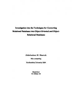
Algorithm
Estimate-
Input
rn
:
are
e : a given
relative
the
1: a given
confidence
has as its value
differences
drawn
from
urn
from
any
a single
(2) The
values
be
points
output
in the
: an estimate
using
index
LNS
approach,
obtained from of
. . .
in
assume point
that
can
to
relation tive
(in also
the
the balls)
present
error-constrained
sampling, can
revised
be compared
index
urn
of
Section special
values
Determining For
database
double designer
the sampling
and
a fixed
tuple ;.~
{Compute
and
if
will
of That
the
rl
>
m :=
the
DBMS
first
step
always sample
For
chooses size for
simplicity,
4.1,
Return
the
LNS
it
Figure
(~
4.1.
uariat ion computing
@,
defined
is specified as u ~ /
the tot al sample
as the Y,
the
size m [Cox
rn,
m,;
(1 – 2(3)2));
m is the
{ adjust
the
ml,
bias)
We tion
r ~ as the
Estimation
Algorithm
Sampling
sample
size,
V2, defined
m ~~:
the
as ~,=,
of the population
sample
‘ (y; – 1)2 /
variance
W2 from
sample.
relative
that
total
is an estimate
the first
Query
Double
step,
can rewrite
error
equation
(4.5)
e and the confidence
in terms
level
of the
I using
equa-
(4.3) as
in Section m = (1)2(1
the error
size m}
Evaluate ad~ltional m – units as the second step
COUNT
size at the first
to compute
from
sample
m;
Using
4.4. When
each
End.
algo-
algorithm,
comparisons
for
t
we
double
we assume
100 tuples
l~i~m,,
~~~,rn yi /
% := N
where
how
m ~ then sample
adap-
so that
the
m
else
is,
a single
using
ILNS
value,
(ball) in m,;
the overall
the
Size
has to determine
number.
of size
basis.
based the first step sample size. It can be determined on precision requirements, experience or, simply, using
step sample
(by
4, we
from
from
Sample
the first
r ~;
model.
Figure
with
y,
sample
rithms. 4.3.1.
and draw relation
Evaluate
can be immediately
only
of COUNT(E);
point
model.
In
meaningfully
size;
population
step sample;
size;
is con-
case
algorithm
to sample
cuts
using
same
(a
files.
of the first
$’:
ml from
of different
the
sampling
and the ball using
that
as far
advantage
are taken
double
variance
sample
Determine
be
index
to
points)
is the underlying the
using
efficiency on
curve
1 at the tails;
Begin
There-
available,
this
the
model
determined the
of are
as LNS’S
remainder urn
(i.e.,
in both
sampling,
just
the
files are used to
equivalent
take
of the normal
Y : an estimate
the
to
relations.
terms files
algorithms the
tuples
V2 : sample
without
has
of view, is
satisfying
constraint.
m : the overall
can
In
a ball
error
level.
SJI-
“ “ . and rm as samples,
compare
space model)
sample
rn
index
error-constrained Hereafter,
as input
Index
point
and
dimensions)
order
in only
the
attributes.
of
files.
size
When model
In
value
rz,
sample
merging
join
index
relations
space
tuples
on the
a sampling
cerned.
evaluating
operand
xl : the first step sample size; y : sample mean of the first step sample;
be
space model
access to the entire
rz,
as the
by
the
using
files
in the point
n
error;
off an area of 1 –
while,
can be drawn
sample
files
fast
fore,
relations
tuples
simply
using
provide
and the urn model. sample tuples can
with
of COUNT(E)
t : the abscissa
mentioning
relation.
of points
expression
worth
of the
sample
obtained
entire
or all
model,
SJI-expression
Each
given
between the point space model (1) In the point space model, the
an
model).
space.
some
E:
point
set of original
e, 1)
relations;
a single
Var There
COUNT(E,
same value
r2, . . .. and
into
of the urn
(i.e.,
of the
say
1 dimensions
have
merged
a ball
the merge
of the values
original
which
are
becomes
after
n –
regardless
values,
then
n – 1 dimensions,
merging
coefficient formula
of
+:)
+ 8(1)2+%
t
e~
(4.6)
ml
mlv
for Note
52] is to thk
be taken
that at
is not true,
ple size is already accuracy,
281
and
m – m ~ is the additional the
second
i.e.,
m ~
large one
step, ml,
enough
can
if
it means to obtain
simply
sample
m >
stop
m,.
that
units When
the sam-
the required the
process
without
going
on to the
estimate
from
the first
result.
Also
larger
one can see from
the
total
fist
sample
sample
estimator
the bias,
as the final is what note
the
That
needed
mean
are
3rd
for
and
term
when known
4th
equations
the
withki
), the
and (4.6).
(4.6) is the sample
equation
(4.4)), (4.6)
and
the
are the
2nd,
select
adjust-
That
may
help reduce Cox
meets
sample
Clearly,
condition.
The
some modifications
(j’
(1-P,)
P1(l-P1)
1 at
the
1 values, However,
can be applied urn
model.
reduce N(p
straint,
on for
a population
sample
size for
(4.6)
estimator Cox
bias,
– (Z)zp
case in the is more
/ (1 – p))
is also slightly [Cox
52]
as the final
proportion
the value ments 4.4.
the
1.
of the
We will
in Section
overall
use thk
formula
tithm
for
of
In thk
we compare
section, sampling
4.1 (i.e., we only
the
Three
algorithm
sample
where
LNS
from
the
Let query
us now consider the select to be estimated is COUNT with
Note
space model
same,
i.e., have
10,000 tuples,
that,
point 1. We
sample
tuples
the
table
thus,
286.
in
[LiNa
y has
to
be
Since the selectivity
size is 1/0.2
sizes
are
0.2. The For a 0.8
follows.
e = 0.1;
con-
are
“ 286 =
1430.
under
the
listed
from
the
the
as well
assumed
that
100 sample
first
100 sample b =1 for
expected
as for
infor-
tuples:
OnA the
tuples,
in LNS
a 10%
sample
double
preliminary V /
Y
algorithm)
error
tuples
and
= for
a 80%
in ILNS
algo-
be 0.8 “ 1430 = 1144. double
first
sampling,
step
with
a sample
and selectivity
0.2,
size of
the
average
overall
sample
size
m is (~)z .,.
(L) 2’
of
+13 (4.6)
is exactly
is the
required
variance
Figure
and ILNS
+
1.28 = 727.
Note
The
second, cost
the
same
term
be
the
and mean. In the example, 10% higher than the sample and is much smaller than
equation
(4.4),
a situation
can
knowing
+ 33~26 in
the
are known,
considered
population
the extra size from those for
which
where
of the population
terms
not
= ~5;
as the equation
size for
mean
third for
+ ‘) 100 the first
that
the
sample
and
extra
0“16 1000.22
as the variance
cost is around equation (4.6), the LNS and
algorithms.
Operator
r is a relation formula,
the
condi-
the same error
as
0.2; and thus
the
ILNS Select
For
selectivity
algorithm,
have
(1 + 8(W)2
algorithms. Since LNS and ILNS algorithms are developed for only select, join and intersection operators, here we only consider these operators. 4.4.1.
algorithm,
1430
sample
ILNS
we
would
level,
our experi-
in
l“~~).
with
the performance
r ~) with
= 655
sample selectivity at the first step is 0.2, With a 10% (e = 0.1) error and a 80% (~ = ~~~ confi~e:;e
Approaches
described
from
the
sizes n.
As for
To
units
under
“ U 0.04
2.6 from
sample
for
100 at the
6.
Comparison
double
sample
figures
With
t p is the
different
to 1 in the stopping
2.6 . 10 “ 11 =
selectivity
take
estimate,
error,
is obtained
and
to
a 10%
confidence,
space
Iiased.
=
with
0.2 - 0.8 / 0.2 = 0.8 (
90b];
52], after
formula
sample
b is equal
has
as
when
(4.6)
wKlch
This
the
For variance
operation,
confidence
e2plml
step.
(i.e.,
equation
model.
[Cox
of the sample
first
performance
O and
in
is written
consider
us consider
for
space model
t2 +———————
p ~ is the proportion
value
m) than
population
the point
3
+
better
population
formula
fol-
an estimate
e = 0.1)
sizes n.
let
column
PI
the
the
formula
as above,
~.
where
the
another
size when
1 values.
thk
about
to obtain
(i.e.,
that
sizes (i.e.,
71
tion
si%e.
52] also provides
the
O and
information the sample
[Cox
computing only
is,
us
. of 0.2 (i.e.. ,,
Now
ment terms (i.e., the extra cost) for not knowing the variance and mean in an error-constrained environment.
let
for a 80%
comparison sample
of 0.8, 0.9, 0.95 and 0.99.
required
the
the the
needed
of 10%
“Reference
selectivity
which
for
tuples)
levels
First, column
0.5)
4.1, we” list
an error
to
Please
and
(i.e.,
of input
confidence
query,
variance
of equation
number
biased;
(4.4)
50%
In Table’
the
m ~.
4.1 returns.
and
lows.
Y(I – 2(e / t)z)
size of the
Figure
0.2)
the
smaller
m >
population
(i.e.,
terms
the
slightly
in equation
the
return
as the final
(4.5) that,
to take
the in
between
is, the first
size
m ~ is,
suggests
algorithm
similarity
and
result
be, assuming Y becomes
Cox
estimate
the
step
equation
size
size m will
The adjust
second
step sample
for
and the urn
each point chosen
a single
or ball the
the
10,000
are exactly
the
there
the value
O or
to be 20%
(i.e.,
has only
selectivities
Counter
operation,
model
Operation
Let
and F is a selection select
Join
4.4.2.
operation, i.e., (ur (r)), where
integers
282
us
consider
ItXr2) tuples, is
Assume For
a single between
the that
simplicity, join
attribute
1 and 10,000.
join
both we
r, also
with
operation and
ra have
assume a domain
that of
We assume Selectivity confidence
=
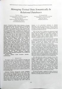
Reference
0.2
upper
LNS
ILNS
Our
bound
the
stopping
Note
that
level
sizes
sizes
sizes
sizes
0.8
655
1,430
1,114
727
not needed
0.9
1,082
2,090
1,672
1,179
is unknown,
0.95
1,537
2,750
2,200
1,661
figures
0.99
2,652
6,100
4,880
2,843
larger
=
the
listed
and y
Reference
I
level
sizes
0.8
164
0.9
271
0.95
384
0.99
663
Table
Sample Error
We have tributions efficiency
have that
bute
value
bute
values
the urn, as t; thus 10,000.
That
dently
27.84 values ball
11.276
normal
(i.e.,
depending are. With
assumption
there
with
Consider variance
10% as
(
peak than
follows.
;)2 (~ “
for
the
in
11.76
LNS)
respectively.
the
and
for
the
Therefore,
a 10% error
same
/ ?
and a 80%
population
is
7962
sampling,
the
expected
.
sample
the
same
error
constraint,
is
( —)2 0.1
“
. (1+8(W)2 1.28 is much smaller
+
u 100.12 than 7962
and ILNS
+
+ ) = 2183, 100 and 3225 required
algorithms. =
11.276
Reference sizes
LNS
ILNS
Our
sizes
sizes
sizes
1,847
7,962
3,325
2,183
3,051
11,637
4,713
3,546
0.95
4,332
15,372
6,226
4,997
0.99
7,477
37,361
1,5132
8,559
Variance Confidence
=
w
11.276
note
are the
attributes of the
2.818
to
Error Table
4.4.3.
equation
ILNS
Our
sizes
sizes
sizes
806
507
1,178
822
1,550
1,157
3,769
1,981
e=lO% Required for the Join
for
the
Desired
Operation.
Operation
the
intersection
operation
is not
dis-
cussed in [UINa 90 b], it can be easily modeled by the urn model or the point space model [HoOT 88, HoO z
1.28),
88].
example,
sizes 9
Sizes
Bound
Intersection Though
for
LNS
few
popula-
0.8 (t =
‘Reference
Sample Error
one.
level
4.2.
values, very
the former
sizes
variances
non-zero
cases where
Reference
levels
the
1270 and 3700 balls
the latter
) = 1847 from
b =
$(~) in LNS)
0.8
join
b values
value
sizes are obtained,
The
the
is
1,0002,
Corresponding ball
having
a confidence
sample
average
b = 27.84
sizes for
double
the aver-
Please
Also,
1,
0.9
value
and the variance
the
Y =
is
than
of
the normally dktributed ball values 11.276. For a given relative error of
(e = 0.1) and expected
with values.
b value larger
on 100 indepen-
of the join
with
the be
in
rllxrz
(i.e.,
much
= 3225.
levels
distribution.
2502 and
are about
deal
has a sharp
the number
mean
to
for
Confidence
respeca ball
attribute
Based
and 2.818).
we
non-zero
1,0002,
of
the
to
Variance
with
are, on the average,
1,0002)
i.e., tion
dktribution
tuples
b the
we attri-
a normal
algorithm,
sample
for the LNS
&k-
attri-
to
on how
Since
dktributions,
/ 27.84)
for
12 w~lch
distri-
join
respectively.
11.276
the
and the join
corresponds
than
11.276
dk-
comparisons,
ILNS
for
and is When
1.28
size,
compare
and the average
distributions
do not
to
to
1).
the same error
that
has
in
size is 1 ‘ 7962 = 7962.
level
As
Operation.
to use normal
be larger
/ 1 (compared
normal
Desired
since normal
the variance
and 2.818,
the
dktributions
values
2502 and two
for
size will 4.2
1 (compared
(11.276
balls
variances
/
algorithm.
= 7962.
As for 11.276
confidence
the Select
have
respectively,
the
the expected
output
of 10,000), have
691
same join
(out balls
1,324
Y is 1.
with
11.76,
values
the above
2,684
is, the population
between (i.e.,
two
2502 and rl
the
respectively;
and
404
a normal
of
of the ball
Mference
550
10,000;
of balls
values
2.818,
1,100
has as its value
have
generated
variance and
ball
of the balls)
attribute
2.818
in rl has a distiict
t in
number
age value
287
to be close to real life
variances
values
total
418
of
1 and
tuple
rz that
836
following
rz have
and the
in
The
the
and
Each
are
chosen
each tuple
5,000,
tively.
177
algorithms,
between of
sizes
286
For
values
For
sizes
572
un~now;
sampling
value
sample
sizes
Required
been claimed
tributions.
tuples
Bound
of different
butions
mean
Sizes
the
expected
Our
e=lO%
arbitrarily
for
ILNS
I
Error
4.1.
assume
LNS
k,
b values
the
the
b, is known 11 b ~ — ~ (— +
is usually
Table
the lowest
i.e.,
y >
sample
in
algorithm,
values,
information
2.6.27.84.10.11 confidence
in LNS ball
in the double
the guessed
known,
0.5
the
concMion
thk
constraint Selectivity
that,
for
To
corresponds is
model
r ~(l rz in
to a tuple
the
rl. A ball has a value 1 if the is also in rz; otherwise, the
(4.4).
283
urn
model,
t in a designated
each
relation,
ball say
corresponding tuple t ball has a value O.
Clearly,
as far
section
is exactly
as the
urn
the
model
same
is concerned,
as selection.
4.1 can be used as a source section operations producing
Thus,
inter-
where
N
Table
points tighter
in the point space. bound on the sample
of comparison for inter2,OOO and 5,000 output
and
Improvement
Using
Sampling In the are taken pling
dkcussions
of Section
replacement
more
implemented
population
pling
size
(i.e.,
simple
From
the
is not
without
variance called
the
very
random
tables, high,
population
sam-
in
i.e.,
size.
large
a factor
finite
the =
simple
by
.
the
N–1
replacement
U:
reduce
called
many
89],
close to
When
compared
to
may
population
required
reduce
of N— m /
the
number
of
(5.3) gives a equation (4.6),
CASE-DB,
correction),
sample
size.
the
When
N
(4.2) should
be written
the
the
time-constrained)
prototype
wKlch
the then,
1. And
equation,
let
is
(SS)
~~~,N(y;
is large,
space limitations,
(4.2). If is used,
imental join
and
6.1.
/
/(
1 +
;(:)’)
consider
for
without
For
a 10% error
the
required
to see
replacement
‘Reference
sim-
can affect
and a 99% sizen
how
for
ran-
from
attributes
of
the
The
and
given
underlying rewrite (N-m)
sampling the
method
equation
s’ /N,
only
replace
where
space)
simplify
the second
s’ is defined solving formula
the
term
sampling,
as ~i=l
‘(gi-~)’
(1 —p J
space model),
(more
accurately,
and
m is the
and
for
third
overall
sample
the
sample
terms
of
-
(N’
+ 2Nz,
+ (Z1 + Z2 + Z3)N2=0
size
equation
size.
To
rn, let
the
(4.7)
Sections sample
2 and tuples
are
each,
section
be
is
4.3
6.2.
+ Nz,)m (5.3)
284
a
to be
number
the
double
fractions just
that,
are drawn
in
are
from the
from
and no index
obtained
r,.
point
(some
or)
files on join
sample
on relations
level
limits for
(e.g.,
the
specified
limit
5%,
10%,
and
sampling
the tech-
of actual errors is to be compared
And the column of runs in which
to be less than e, which
confidence
of
a
and
level
level
Input
or equal
1% the to
is to be compared 1 (in
95%). Creation
for
95%)
the column f% gives the averfrom each input relation. The
are found error
2%,
different
e% gives the average during 200 runs, wldch
errors
experiments.
to sbowj
always
confidence
with
in the tables
200
designed
(here
errors, sizes
value
from
been
error
actual
specified
with
for
performed
have
relative the
always
as
is defined
not
and each data
confidence
relative
the following
tuples
to the total
relations,
with the specified error limit. gives the ratio of the number the
wKlch
sampling
relations
experiments
column observed
the
experimenexpressions
of
Furthermore,
niques. In the tables, age sampling fraction
by ((N–m) / N) (l–PI), where N is size (i.e., the number of points in the
equation
this
required
one
and
algebra
of tuples
all the input
tuples
etc.),
select,
CASE-MDB.
are needed.
different
U2 by
for m. As for equation for a population with
z 1, X2 and ZS~ respectively. BY solving quadratic equation, m can be obtained. (N+z,)m2
as
replaci?~~the
O and 1 (e.g., the point
term PI (l–PI)) the population point
for double
(4.6) by first
/ (m – 1), and then (4.7), whkh is the values
replacement
in
number
equal
Experiments 10,000
the
~ as the measure,
approach,
Recall
the exper-
size, we choose to use the samp-
in a relation.
from
to
on single
operations
using
of tuples
ple
without
of
of the number
drawn
as
Due
Experiments
of the sample
fraction
such
90].
the ratio
sampling without replacement is 7,477 / 7,477 (l+— ) = 4278, which is much smaller than 10,000 7,477 from Table 4.2. Similarly, one can use the simsampling
of
we present
sampling
relational
in [Dogd
all of the operand
dom
random
of (or
management
tuples.
operations
arbitrary
space model,
confidence simple
version
real-time
techniques
paper,
projection
for
sampling
an example
sampling
the efficiency. level,
(5.2) e
We now ple random
memory
sample
double
intersection
Instead ling
ey
[Liu
estimation
database
draw
in this for
Design
be
measure
~ = p)’
query
disk-resident,
sampling
to
results
can be found
– ~)’
are
systems,
CASE-MDB
is a main a
as other
sampling)
Estimators
(4.4) will
and
prototype
(as well
cluster
may
as
S2 be
the equation
89]
COUNT
is
sampling
management
system. Double sampling implemented in CASE-DB random sampling and CASE-MDB uses simple without replacement (SRS) and systematic sampling
(5.1) TO simplify
[HoOT
CASE-MDB
CASE-DB
adaptive
database
error-constrained
tal results
N–
and
two
CASE-DB for
purposes.
sample
and thus,
sampling into
the
N— 1 (wVlch
N. Let us consider the equation random sampling without replacement
equation
first,
i.e.,
Equation size than
Results
Double
sample size, a better choice is to use simple random sampling without replacement. Simple random sam-
can
size,
in
Experimental
incorporated
4, all the samples
sizes can be very
than
6.
Random
Replacement
replacement). sample
even
Simple
Without
with
with
cases, the or
is
population
DBMS.
tuples. 5.
is the
Relations
this
section,
Each with
input
integer
unique
relation
values.
random
from
numbers
another.
interest the
in
The
the
selection
observe
the
we have
second
attributes
chstribution.
the
or
the
using
experiments with we use
dMerentiate tuples,
to
ordered
and
relations
with
in which
or a normal of the
techniques,
relations
respect
double we have
in wKlch
the
in To
second
unordered
ordered
Experiments on a and Join Operations
1%
f%
‘I’he
with
fraction
used
total far
relation as the
tuple actual
97
100
0
95
100
0
100
10%
14
4
96
28
3
100
20%
4
8
97
I
Given
Error
Selection
85
Systematic
in
step
the
the
sampling
values
every
tuple
equal
ordered
e%
1%
f%
e%
2%
50
2
0
50
2
0
5%
38
4
83
38
49
6
10%
14
4
91
14
10
20%
4
8
98
definition, simple
the
any
significant
sample
influence
taken
sampling.
columns
fractions for different For simple random values
computed
error
Table
close
equation
experimental
0.2 from
relative sampling
quite
from
10% relative the
are
the
1%
f%
e%
l%_
1
96
100
0
100
5% 10%
14
2
94
42
1
100
4
4
97
11
2
100
20%
2
5
100
3
5
100
6.1,
and
it
gives
average
by
f%
This
means
exactly
that
double
sampling
(5.3).
For
example, confidence for
computed
as the formula
sampling
without
f%
1
e%
1% 100
2%
48
1
94
49
1
13
2
98
13
3
a
5% 10%
4
4
97
41
100
In sys-
20%
100
20
100
26
Selectivity
80
Table
Select Operation
6.2.
number
0.5;
with
for
ple, if the sampling
fraction
where
a
samples of k
the has
Therefore,
level,
Selectivity
chosen
dered,
number
to use a cut
when the systematic
of simple
of 0.5.
pling
(5.3) specifies.
Of
285
a limited
is 10%,
there
A typic~l , k -t 20
possible
of underlying
10
sample may , , tuples, 1~ks
10.
is determined
samples.
We have at 50% 50% for is unor-
should
are (more
in general, be similar whether
sampling
exam-
arc only
valnes,
of an estimate
on the
For
sampling fraction is larger than When the relation sampling.
tuples
course,
10
only
fraction
Therefore,
behaves
only
(SS),
can be drawn.
cafi be dra~~. ,k+lo k
the precision
by a limited
is also
sampling samples
consist
values
systematic
of possible
possible
selectivity
value
on top
replacement
=
tables
14%. Also, the confidence levels (i.e., 1% columns) are quite close to the specified confidence level 95%. random
1%
is a
of sampling
expected
95%
ordered
e%
ord-
a bad
in
the
size is 14%
Sampling
unordered
Error
sampling
to
the
Systematic
Given
errors (e.g., 2%, 5%). without replacement,
and a given average
Sampling
unordered/ordered
of m tuples
is observable
give
of 0.2.
e%
For f%
Selectivity
Adaptive
SRS
is a good representa-
otherwise,
with
49
a
has
the systematic
phenomenon
Operation
a
into
ordering
a sample
Select
f%
6.1 and 6.2.
these
== 0.2
2%
has an Thus,
combination
population,
in
of the storage
storage
estimate;
Thk
The
100
because
m tuples
on systematic
When
a precise
estimate.
of tuples
as a sample.
every
a
affect
to be selected
regardless
not
of the whole
gives
51
48
unordered/ordered
the
random
performance of
6.1.
Error
values
simple
ordering
chance
the
either
not
of size m randomly
sample,
can be drawn. tive
1%
I
Given
Therefore, will
For
on the
be selected
sampling,
they
combination
However,
tematic
storage
effect
to
random
ering.
since
Table
As
or it does not; of attribute
88].
has an equal
chance
Sampling
unordered
I
of the
here).
are not important.
[HoOT
every
2%
is concerned,
formula
operation
no
and
is always
the distributions
(SRS), has
J
The sampling
or 200 tuples
estimator
performance
sample,
= 2%
the selection
selection
relation
first
j
COUNT
attribute
the
98
—
f%
to
on a selection
0.2 and 0.5.
we do not discuss for
are performed
selectivities (i.e.,
satisfies
100
1
j
Operation
experiments
operator
1%
2
Selectivity Selection
6.3.1.
I
e%
39
unordered
Single
e%
80
respectively.
6.3.
Sampling
unordered/ordered
2%
attribute.
and
Adaptive
5%
tuples
relations
SRS
unordered/ordered f%
attribute
relations
behavior
sampling with
E Error
of
attribute. of
Given
tuple one
involved
join
a uniform
the
Wferent
attribute
with
either
observe
also run
one is the
distributions
experimented
sampling
Hereafter,
the
both contains
dMerentiate
i.e.,
have
attributes,
attribute
attribute
query,
To
ordered
to
formula of
two
first
second
effect
values,
are
has
The
or less) randomly the results to this
for
simple similarity
distributed.
systematic
random occurs
sam-
sampling. or
not
depends
on
how
structed.
Thk
sampling
there
than
95%
those
observed
at
ples have that
others
the
mates
are very
are very
sampling.
precise
smaller error a higher
the
required
f%
sample
than
having
72,750 =
10,000 are
drawn
for
that
level,
no
large
for
the
each.
in
the
effort,
We assume
point operand
of sampling,
and thus
DB
and
CASE-MDB.
Note
the
latter
5002
does not
have
estimator.
shown
that
relation
that
corresponds
0.052) of the point
cuts
down
produced
relation
attribute
join
are
not
uniformly
values
each row/column
will
1.
by a tuple
Since
have
though
the
independent]
y drawn,
the
bute
and thus
the distributions
1, will
mates. obtained
have
dktribut
an effect
on the
in, say,
ordered
number
varithk
of under-
Ss ordered
unordered 1%
f%
e%
1%
f%
e 70
2%
39
1
99
39
1
100
39
16
5% 10’% 20’%
19
1
99
19
1
98
19
5
53
10
3
100
10
2
100
10
3
99
5
6
100
6.3.
56
Join Having
=
1%
12
56
100
100
0.00073
Operation with Join Uniform Distribution.
Attribute
eYo
I%
f%
2%
38.7
1
92
5%
18.5
2
10%
10.3
20%
5.0
longer
of join
attri-
1%
f%
e 70
38.7
1
99
38.8
29
92
18.5
2
%7
18.5
8
5
4
97
10.3
3
98
10.3
7
91
8
95
60
6
100
5.0
3
100
Join Having
=
0.00073
Operation with Join Normal Distribution.
Intersection
butes,
the
with
guarantee we take
of points
of points
6.4.
ordered
e%
Attribute
Operation
Intersection operation can be considered as a special case of the join operation in which all the attributes (or the key attributes) are ‘joinm attri-
r ~ and If
Ss unordered
I
f%
of
no
precision
SRS
I unordered/ordered
Table
dktributed, are
ions
to
a large earlier,
sampling.
Selectivity
frac-
a s~mple
number
points
applied
SRS
correla-
operation.
different
sample
are are
e%
6.3.3.
the
there
and some that
limited
for systematic
with
in the selection
tends to give we explained
unordered/Ordered
Error
space.
r2 in
high
is due to having
Given
Consider the point space of a join operation The number of points with value 1 on the row (or the same column) represents the of tuples
to those
f%
in CASE-
sample
to
the relations
close
sampling
operations As estimates.
samples
Table
on the performance a 5%
size.
empirical
are ordered,
are very
Systematic
in
when
are
the relations
that
Selectivity
of
with
the introduced
note
to
same
in our
as explained
in join
and
Clearly,
is adopted
effect
low.
sampling, results
sampling,
When
Error
88, HOOZ
tremendously
a severe Also
each
values,
random
the
the first
one pair
even
of the
severe
larger
compared
correlated
[HoOT
that
correlated,
points
are not
systematic
ordered,
Given
are drawn randomly, the sample points independent. The experimental results
in [HoO z 88] have
value
effects
are
be obtained
independent
Thk from
500 tuples
to
points may
attri-
relations
that
relations.
cost
entire
the
one can construct or
corresponds
the
number
However,
lying
selectivity
With
space
same
(i.e.,
sample
the join
than
each relation,
relation, points,
the
sample tuples are no longer
i.e.,
available.
point
dMerent
from
with
phenomena
operation
operand
is 5% from files
each
from
0.25%
the
in estimation
a sample
ance
is
same
obtained
on a join
with
sample
in which
of the
dktribution.
tuples
sampling
is Elgher
samples
tuples,
each operand
points
tuples
space when
a uniform
very
sam-
unnecessary.
0.00073
index
from
sample
the point
simple
adaptive
adaptive
evenly
have
operation.
sampling
distri-
I is more
over
values
As for
esti-
double
normally
value
dktributed
are not
estimates
and
w~lch
considered
fraction
independent
value
the
the
sampling,
output
tuples
sampling
with
why
are performed
= 72,750/10,0002
join
good
explains
from
with
evaluations.
Operation
producing
the
are not
This
sampling)
Note
and
Experiments
r ,(X Irz. same
samples
sizes for double
confidence 95%
Join
tion
as sam-
sampling.
6.3.2.
tion
selectivity
than
points
bute
variance
that sam-
some other
columns
adaptive
to unnecessarily
adaptive
88],
same for
in others
random
constraint.
has
500
to
the
Since
are cases where
while
compare
Clearly,
given
there
the
while
there
simple
much
step
lower
close
since
some estimates
(using
is due
much quite
distributed
buted,
sampling.
population.
&2
uniformly
con-
bad.
We now pling
random
underlying
of the
6.1 and
are
are ordered, it is possible fraction, the underlying
relation
fractions,
representatives
1% values
1% values
(or almost)
entiie
samples
in the case of systematic
with
in simple
exactly
in tables
why
the tuples sampling
of the
pling
underlying
are cases with
and
When a certain
the
explains
than at bute
of esti-
a higher one
first
step
with
different since
selectivity.
some points
operation.
point
to discuss values,
a low
we have
in the join most
have
with
probably that
each
sampling Each
value
distributions ‘join!
order
we
1,
(10%)
or column
Here!
to
the value
fraction
row 1,
In
with
has
do not
of njoin m attriattribute
value
is
unique in a relation. Systematic sampling has a poor performance especially when tuples are ordered.
This explains why a better performance is from relations with join attribute values
286
1%
0
be worked
out.
More
importantly,
of the bias is unknown, Ss
SRS
Given Error
e Yo
f%
1%
f%
0
100
50
1’%
I f%
e%
1%
2
40
39
118
0
100
6% 10’%
76
1
99
60
2
100
19
159
0
50
3
98
48
4
100
11
108
0
20%
30
6
99
30
7
85
10
188
0
Table
Sampling
6.5. Intersection Tuples.
Fraction
Operation -
[Coch
77]
[Cox
52]
10%
=
with
w.
Cochran,
Ed.
John
D.R.
Cox,
[Dogd
90]
E.
!! Sampling Wiley
Dogdu,
I
Error
I
unordered/ordered
unordered
ordered
[HOOT
1%
f%
e%
1%
f%
e%
1%
2%
91
0
100
50
2
48
39
118
0
6%
57
1
100
50
2
100
18
145
0
10’%
35
3
100
35
16
38
10
183
0
20%
20
5
100
20
9
94
10
183
0
=
Hou,
G.
6.6.
Intersection tuples.
Operation
W-C.
89]
Hou,
with MOD, [HoOZ
88]
COUNT(E)
query
The
without We
error
very
bound
[LiNa
well
with
We
have
89]
also
LNS
R.
an additional
sample of sample
these
approach, denoted
te8ted,
we propose.
bias
there
with of the
by
n .slm
in
estimator
least than
the
adaptive
estimator
double
the
n s/m is basically the same Y, in [HoOT 88, HoOT 89]. when
the
sample
size is
magnitude
in
of
the
checking
the number
ing whether
how
the
bias
sample of output
an ad<ional
is actually
the
estimator,
units tuples
sample
unit
are
which
taken
(e.g.,
and then
decid-
is to be taken
how the bias is introduced),
J.
Algebra
ACM
Naughton,
TODS,
sub-
“Estimating
Transitive
Naughton,
the The
“Query
.,
Naughton
and
Sampling ‘A
Memory
Management
EstiACM
D.
Schneider,
Estimation ‘! , ACM
Main
Size
Sampling”,
Selectivity
Y-M
The
Closures”, Amsterdam,
Adaptive
J.
through
SIGMOD,
1990,
Real-Time
Data-
System--Implementation 11, MS
Experiments
p,
Sukhatme,
India
and
Iowa,
1984.
A.
67]
T.
needs to
287
etc.,,
Thesis,
“Sampling
Applicationfl,
Wald,
Yamane,
Prentice-Hall,
size
become biased in an error[COX 52, Coch 77]. The
on
[Yama
w~lch is 90, LNS 90].
89, LiNa
45]
the
sampling for
1990.
Lipton,
Hypotheses
query,
[LiNa
is unliased
depends
[Wald
shown
under
PODS,
veys
by observing
prefixed; however, it may constrained environment
- this
[Sukh 84]
are some problems
the
Select-Join(-Intersection)
Note that the estimator as the one, denoted by The
at
“Statistical
CWRU,
July
1989.
or not
We have
worse
Also,
to be solved e.g., the
whether
SIG-
1989. and by
and
compared
in
Conference,
mation
Liu,
Queries
Relational
appear
J.
VLDB
base
estimation
is to be taken perform,
89]
Taneja,
ACM
Ozsoyoglu,
Generalized
Adaptive
[Li”
B.
1989,
G.
to
!Ipractical
we
and
Aggregate
and
of
Lipton
R.
CASE-DB.
and
tuples.
90]
[LNS
plan.
results
called
determine
output
we have
remain the
sampling
COUNT(E)
unit
approaches
assumptions
of
and
sampling
experimental
TX,
1988.
Lipton
R.
confidence
consistent,
implemented
90]
guaran-
random
DBMS
approaches
the number
that
the
[LiNa
the (I)LNS algorithms based on adaptive Given an error constraint and a confidence
the
sampling
and
as the underlying
error- constrained
approach, sampling.
a 8pecified
simple
on our prototype
another
that
with
also presented
performed
sampling-based that
Austin,
Constraints”,
and for
Expressions”,
5,OOO Output
approach
is unbiased
replacement
have
level,
estimation
estimates
performs
a double
Taneja, Algebra
Relational
OR,
Netherlands,
tees a desired level.
Time
Hou
Size
presented
B.
PODS,
G. Ozsoyoglu
Portland,
W-C.
7. Conclusions have
Double
Relational
Aggregate
Hard
15th
We
and
for
ACM
“Processing
10%
with
on
Manuscript,
Ozsoyoglu
Estimator
mitted
Table
results
Unpublished
Estimator
Fraction
sampling!!,
1988.
e%
Stage Sampling
double
‘Experimental
Expressions”,
f%
First
by
1990,
W-C.
Ss
Third
1977,
39.
CWRU, 88]
Techniques!’,
Sons,
‘Estimation
‘Statistical
SRS
&
samplingfl,
2,OOO Output [HOOT
Given
also
8. References
Biometrika,
Stage
will
ordered
e%
2%
First
magnitude
levels
be inaccurate.
unordered
unordered/ordered
if the
the confidence
Iowa
State
!Iseq”ential ‘,
Theory
Third
Ann.
, 1967.
of
New
Univ.
Tests Math.
‘Elementary Inc
Ed.,
Press,
of
Stat. Sampling
Vol
Sur-
Delhi, Ames,
Statistical 16,
1945.
Theory
!’,