Error correcting codes and spatial coupling

Error correcting codes and spatial coupling Rafah El-Khatib1 , Jean Barbier2 , Ayaka Sakata3 , and R¨ udiger 1 Urbanke 1

arXiv:1409.7465v1 [cs.IT] 26 Sep 2014

2

EPFL, Lausanne, Switzerland Ecole Normale Supérieure, Paris, France 3 RIKEN, Wako, Japan

These are notes from the lecture of R¨ udiger Urbanke given at the autumn school ”Statistical Physics, Optimization, Inference, and Message-Passing Algorithms”, that took place in Les Houches, France from Monday September 30th, 2013, till Friday October 11th, 2013. The school was organized by Florent Krzakala from UPMC and ENS Paris, Federico Ricci-Tersenghi from La Sapienza Roma, Lenka Zdeborová from CEA Saclay and CNRS, and Riccardo Zecchina from Politecnico Torino.

Contents 1 Polar Codes 1.1 Motivation . 1.2 Upper Bound 1.3 Lower Bound 1.4 Summary . .

. . . .

. . . .

. . . .

. . . .

. . . .

. . . .

. . . .

. . . .

. . . .

. . . .

. . . .

. . . .

. . . .

. . . .

. . . .

. . . .

. . . .

. . . .

. . . .

. . . .

. . . .

. . . .

. . . .

. . . .

. . . .

. . . .

. . . .

3 3 4 4 11

2 Applications 12 2.1 Metrics . . . . . . . . . . . . . . . . . . . . . . . . . . . . . . 14 3 Low-Density Parity-Check Codes 3.1 Linear Codes . . . . . . . . . . . . . . . . . . . 3.2 MAP decoding . . . . . . . . . . . . . . . . . . 3.3 Low Density Parity Check codes . . . . . . . . 3.4 Configuration model . . . . . . . . . . . . . . . 3.5 From Bit MAP to Belief propagation decoding 3.6 Asymptotic Analysis: Density Evolution (DE) . 3.7 EXIT curves . . . . . . . . . . . . . . . . . . . 3.8 Some basic facts . . . . . . . . . . . . . . . . .

1

. . . . . . . .

. . . . . . . .

. . . . . . . .

. . . . . . . .

. . . . . . . .

. . . . . . . .

. . . . . . . .

. . . . . . . .

14 14 15 15 16 17 19 20 23

4 Spatially Coupled Codes 4.1 Protographs . . . . . . . . . . . . . . . . . . . . . . . . 4.2 Construction of Spatially Coupled Codes . . . . . . . . 4.2.1 Protograph construction . . . . . . . . . . . . . 4.2.2 Random construction . . . . . . . . . . . . . . 4.3 Why spatial coupling . . . . . . . . . . . . . . . . . . 4.3.1 Degree dependence of the uncoupled ensembles 4.3.2 Spatial coupling might help . . . . . . . . . . .

. . . . . . .

. . . . . . .

. . . . . . .

. . . . . . .

23 24 24 25 25 26 26 28

5 Density Evolution for Coupled Codes 28 5.1 Summary . . . . . . . . . . . . . . . . . . . . . . . . . . . . . 32 6 Threshold Saturation 6.1 Proof by Maxwell construction . . . . . . . . . 6.1.1 Definition of area threshold Area . . . . 6.1.2 Existence of a special fixed point . . . . 6.1.3 Saturation . . . . . . . . . . . . . . . . . 6.1.4 Convergence . . . . . . . . . . . . . . . 6.2 Proof by EXIT charts . . . . . . . . . . . . . . 6.2.1 EXIT charts . . . . . . . . . . . . . . . 6.2.2 Proof by EXIT charts for coupled code 6.3 Proof by Potential Functions . . . . . . . . . . 6.3.1 Potential Functions . . . . . . . . . . . . 6.3.2 Potential Functions for coupled system . 6.4 Summary . . . . . . . . . . . . . . . . . . . . .

2

. . . . . . . . . . . .

. . . . . . . . . . . .

. . . . . . . . . . . .

. . . . . . . . . . . .

. . . . . . . . . . . .

. . . . . . . . . . . .

. . . . . . . . . . . .

. . . . . . . . . . . .

32 33 34 35 36 37 39 39 40 43 43 43 44

Figure 1: A transmission scheme of scalar quantities over the binary erasure channel with parameter .

Figure 2: A transmission scheme of vector quantities over the binary erasure channel with parameter .

1 1.1

Polar Codes Motivation

Consider the transmission scheme depicted in Fig. 1 where one bit x ∈ {0, 1} is sent over a channel that either erases x with probability (w.p.) or passes the bit unchanged w.p. 1 − . This channel is called the Binary Erasure Channel with parameter and we will denote it as BEC(). The receiver thus receives the symbol y ∈ {0, 1, ?} where ( x w.p. 1 − , y= (1) ? w.p. . We want to recover the transmitted bit at the receiver and for this purpose the receiver forms an “estimate” of x given the received symbol y, denote this estimate as x ˆ(y); our goal is to minimize the quantity Pr({ˆ x(y) 6= x}), i.e., we want to minimize the probability of error. If we are only sending a single bit then we cannot hope to estimate the transmitted bit reliably in case it was erased. There is simply not enough information available. The picture changes if we are sending a block of bits. Consider therefore the slightly more general setting shown in Fig. 2 where a vector x ∈ {0, 1}n is sent on the same channel, the BEC(). At the receiver, the vector y ∈ {0, 1}n is received such that each component of this vector follows the rules in (1), i.e., each component is erased independently from all other components with probability . It is easy to determine the expected number of erased and non-erased bits for this scenario, namely E[|{yi =?}|] = n, E[|{yi 6=?}|] = n(1 − ).

p The standard deviation associated to these values is σ = n(1 − ). Similar to before, we are interested in determining the transmitted vector x 3

ˆ (y), given the received vector y, and for this purpose we form the estimate x and, as before, Pr({ˆ x(y) 6= x}) is the probability of error. If this probability of error is “small” then we say that we achieve a reliable transmission. It is now natural to ask the following question: how many bits can we reliably transmit over such a channel, measured as a function of the vector length n, when n → +∞? We derive first an upper bound and then a matching lower bound.

1.2

Upper Bound

Assume that we are aided by a genie that tells the transmitter the positions that will be erased ahead of time. More formally, let S ⊆ [n] be the set of erasures and assume that we know this set before sending the vector x. Some thought then shows that the optimal strategy consists of sending our information in the positions [n] \ S and to fill the positions S with dummy bits. The receiver then simply reads off the positions in [n] \ S to recover the transmitted information and this way estimate at the receiver is perfect and we never make an error. This is also clearly the maximum amount of information that we can transmit reliably in this scenario. Since E[|[n] \ S|] = n(1 − ) it follows that the fraction of channel uses on which information can be sent reliably is equal to 1 − . This fraction is called the “transmission rate” and the highest possible rate for which reliable transmission is possible is called the “capacity.” Since we have just shown that the capacity of the genie-aided transmission is 1 − it follows that the real capacity (i.e., the capacity without the genie) is at most 1 − .

1.3

Lower Bound

To prove that the capacity is equal to 1 − we now derive a matching lower bound by describing a scheme which allows reliable transmission all the way up to a rate of 1 − . The typical way to prove this lower bound is by using a so-called “random coding” argument. This argument proceed by showing that “randomly” chosen codes from a suitably defined “ensemble” of codes work with high probability.1 This argument has the advantage that it is relatively simple and short. But on the downside, the argument is nonconstructive and in addition does not take the complexity of the scheme into account. Instead, we will describe an explicit scheme which in addition is also of low complexity. It is called the “polar coding” scheme. This scheme is fairly 1

A code is a subset of the set of all binary n-tuples and typically this subset is chosen in such a way that the individual codewords are well separated. This ensures that even with some of the components being erased, the receiver can still figure out which of the codewords was sent.

4

Figure 3: A one-step polarization transformation for the BEC()’s. recent but the basic idea has already proven to be fundamental in a variety of areas [E. Arikan, 2008]. Let us first make an observation. For the BEC( = 0) the capacity is 1 − = 1. That is, we can fill in the entire vector x with information bits and recover them reliably. If, on the other hand, the erasure probability is = 1, then the capacity is 0 and there is no use of sending any information in x. Both of these cases are thus easy to deal with in the sense that we know what to do. This observation extends to cases where ∼ 0 and ∼ 1. More precisely, we lose very little in the case when ∼ 1 by not using the channel, and if is very small (compared to n) then we can still use all components of the block and most of the time the whole block will arrive without erasures. Only once in a while will we not be able to recover the block, and this simply results in a small probability of error. Let us now introduce the basic idea of polarization. Consider the transmission scheme in Fig. 3. Two bits, call them U1 and U2 , are chosen uniformly at random from {0, 1} and are encoded into two other bits, denoted by X1 and X2 ∈ {0, 1}, as follows (all operations are over the binary field): X1 = U1 + U2 ,

(2)

X2 = U2 .

(3)

Equivalently, we can describe this relationship in matrix form, 1 0 U1 U2 = X1 X2 . 1 1

Assume that we receive Y = (Y1 Y2 ) and that we want to estimate U1 given Y = (Y1 Y2 ), where U2 is unknown (and has a uniform prior). We denote by ˆ1 (Y) this estimate. Note that from (2) we know that U1 = X1 + U2 (there U are no signs in the binary field). If we combine this with (3) we see that U1 = X1 + X2 . Note further that Y1 and Y2 are the result of transmitting X1 and X2 , respectively, through independent erasure channels. We therefore see that we can reconstruct U1 if and only if neither Y1 nor Y2 are erasures, so that X1 = Y1 and X2 = Y2 . Hence, we have ( Y1 + Y2 , if Y1 6=? ∧ Y2 6=?, ˆ U1 (Y) = ?, otherwise. 5

Note that the bits X1 and X2 are sent over independent erasure channels and that P r({Y1 =?}) = ,

(4)

P r({Y2 =?}) = .

(5)

Therefore, ˆ1 (Y) = U1 }) = P r({Y1 6=? ∧ Y2 6=?}) = (1 − )2 , P r({U ˆ1 (Y) =?}) = 1 − (1 − )2 = (2 − ) > . P r({U As we can see, the probability that U1 is erased is strictly larger than (unless = 1). So this does not seem to be a very good scheme. Why then would we use this transform, which is called the polar transform? As we will see shortly, estimating the bit U2 is in fact easier than the original problem, and estimating the bit U1 is more difficult as we just discussed. The key point is that both of these tasks are closer to the two trivial scenarios ( = 0 and = 1) and by recursing this transform we will be able to approach these trivial cases closer and closer. Once we are sufficiently close no extra coding will be necessary since we know how to deal with these two cases. Let us now look at the problem of estimating U2 . For this task, we will assume that a genie tells us the true value of U1 . We will soon see that in fact we have this information at the receiver as long as we decode the various bits in the appropriate order. Therefore, this assumption is in fact realistic. Let us summarize, we want to estimate U2 given U1 and Y. Reconsider our two basic equations. First, rewrite (2) as U2 = X1 + U1 and note that by assumption U1 is known. Further, write (3) as U2 = X2 . We therefore see that we have two estimates of U2 available at the receiver and that these two estimates are conditionally independent since X1 and X2 are transmitted over two independent channels (and U1 is a known constant). We conclude that we will be able to recover U2 as long as at least one of Y1 and Y2 are not erased. Let us summarize, we have   if Y2 6=?, Y2 , ˆ2 (U1 , Y) = Y1 + U1 , if Y2 =? ∧ Y1 6=?, U   ?, otherwise, and

ˆ2 (U1 , Y) =?}) = 2 < . P r({U

(6)

Assume now that we estimate U1 and U2 successively using the following estimators. ˆ1 = U ˆ1 (Y), U ( ˆ ˆ ˆ2 = U2 (U1 , Y) U ? 6

if U1 6=?, otherwise.

Figure 4: A transmission scheme equivalent to the one-polarization step of two BEC()’s. Then, ˆ1 (Y) =? ∨ U ˆ 2 (U ˆ1 (Y), Y) =?}) = P r({U ˆ1 (Y) =? ∨ U ˆ2 (U1 , Y) =?}) P r({U (7) ˆ1 (Y) =?}) + P r({U ˆ2 (U1 , Y) =?}) ≤ P r({U = (2 − ) + 2 = 2.

(8)

This has the following interpretation. In terms of this union bound, the successive decoder is as good as the scenario shown in Fig. 4, where we have two independent BEC’s with different parameters. The scheme in Fig. 3 is obtained from that in Fig. 1 using the following relationship. Given two BEC’s with parameter each, we obtain a BEC with parameter (2 − ), which is called the “– channel” and a BEC with parameter 2 , which is called the “+ channel”. Note further that the sum of the capacities of these two channels is 1 − (2 − ) + 1 − 2 = 2(1 − ). In other words, the average capacity of these two channels is equal to the original capacity. So we have lost nothing in terms of capacity by using this transform with the particular successive decoding algorithm. If we look at the transform itself this is not to surprising. After all, this transform is invertible, and hence lossless. Consider the scheme in Fig. 3 with = 0.5. Then the equivalent scheme in Fig. 4 consists of two cascaded channels BEC(0.75) and BEC(0.25). Notice that the average erasure probability over the two channels is 0.75+0.25 = 2 . This procedure of starting with two independent channels, combining them, and then separating them again into two channels constitutes one “polarization step”. Rather than performing only a single step, we can now recurse. Let us look explicitly at one further step, as shown in Fig. 5. Note that in the second step we combine “like” channels and that we decode successively in a very particular order, namely U1 , U2 , U3 , U4 . The erasure probabilities that we get for the four resulting “synthetic” channels are as follows: • U1 “sees” the BEC w.p. δ(2 − δ) where δ = (2 − ). • U2 “sees” the BEC w.p. δ 2 where δ = (2 − ). 7

Figure 5: A two-polarization step of four BEC()’s. • U3 “sees” the BEC w.p. δ(2 − δ) where δ = 2 . • U4 “sees” the BEC w.p. δ 2 where δ = 2 . Clearly, we can recurse this procedure n ∈ N times to create from 2n = N independent channels with parameter , N “new” (sometimes called synthetic) channels with parameters i , i ∈ 0 . . . N − 1. The parameters evolve at each polarization step according to the rules z → z(2 − z),

(9)

z → z2.

The evolution of the erasure probabilities upon this recursion can be seen as an expansion of the tree diagram in Fig. 6. Notice that the mean of each column, with respect to the uniform distribution, is constant, namely equal to . This is true since z 2 + z(2 − z) = z. 2 This implies that the overall capacity stays preserved. Recall now the motivation for using this transform. We know how to deal with trivial and perfect channels and we hope that by applying a sufficient number of these transforms the resulting synthetic channels will all either become trivial or perfect. If this is indeed the case, and since we know that the overall capacity is preserved, it must be true that the proportion of perfect channels is equal to the capacity of the original channel. Therefore, if we send our bits over the perfect channels and fix the trivial channels to some known value we will be able to transmit reliably arbitrarily close to capacity. It remains to show that this “polarization” of the channels towards these extreme points is indeed the case. 8

Figure 6: A tree diagram that tracks the erasure probabilities obtained by polarization. Towards this goal, let us look at the second moment associated to this transformation ρnn , ρ2n =

z 4 + z 2 (2 − z)2 = z 4 + 2z 2 (1 − z). 2

Consider f (z) = z 4 + 2z 2 (1 − z) − z 2 = z 2 (z 2 − 2z + 1) = z 2 (z − 1)2 which represents the difference of the second moment after the transform and before the transform. Fig. 7 shows the plot of f (z). Note that f (z) > 0, z ∈ (0, 1), and that f (0) = f (1) = 0. This means the following: Consider the nth column and let µn and ρ2n denote the mean and second moment, respectively. We have seen that for n ∈ {0, 1, . . . } = N, µn = , ρ2n is increasing and ρ2n ≤ 1. Thus, lim ρ2n = ρ2∞ exists. Note further that as long as a non-zero proban→+∞

bility mass lies strictly bounded away from 0 and 1, then the increase in the second moment is strict. It is therefore clear that the limiting distribution must be the one where all the mass is located either at 0 or at 1. This is made precise in the following statement. Let znj , j ∈ {1, 2, . . . , 2n }, denote the 2n numbers in the nth column. For δ ∈ [0, 12 ], define Sn (δ) = {j : δ ≤ znj ≤ 1 − δ}. Then for any δ > 0,

lim |Sn (δ)|2−n = 0. In words, all but a sublinear

n→+∞

fraction of channels is either “good” or “bad”. For a fixed δ > 0, we call a channel “good” if it belongs to the set Gn (δ) = {j : |znj | < δ}, and “bad” if it belongs to the set Bn (δ) = {j : |1 − znj | < δ}. Fix δ ∈ [0, 12 ]. Since lim ρ2n = ρ2∞ exists, then for all ∆ > 0, there exists n0 ∈ N so that n→+∞

ρ2n > ρ2∞ − ∆ min{f (δ), f (1 − δ)} 9

6 · 10− 2

f (z)

4 · 10− 2

2 · 10− 2

0

0

0.2

0.4

0.6

0.8

1

z

Figure 7: The plot of f (z). for all n ≥ n0 . We claim that for all n ≥ n0 , |Sn (δ)|2−n ≤ ∆. Since this is true for all ∆ > 0, the claim will follow. Assume that |Sn (δ)|2−n > ∆. This means that there are at least ∆2n numbers znj in the range [δ, 1 − δ]. It follows that the second moment must go up in the next iteration by at least ∆ min{f (δ), f (1 − δ)}. But this would imply that ρ2n+1 > ρ2∞ , which is a contradiction. A more careful analysis shows that, for 0 ≤ β < 12 , with N = 2n , we have βn

lim |Sn (2−2 )|2−n = 0,

n→+∞

βn

lim |Gn (2−2 )|2−n = 1 − ,

n→+∞

βn

lim |Bn (2−2 )|2−n = .

n→+∞

This gives rise to the scheme shown in Fig. 8. Consider a polar code that is polarized n times, where n is chosen to be “sufficiently” large. The code thus has 2n channels, input bits U1 , . . . , U2n and output bits Y1 , . . . , Y2n . “Freeze” the channels j ∈ Bn and put the information bits in the channels j ∈ Gn . Here “freezing” means that we put a fixed value in these positions and this value is known both to the transmitter as well as the receiver. In fact, we are free to choose the value and generically we will choose this value to be 0. Decode the bits U1 , . . . , U2n successively from 1 to N . Of course, if a bit Uk is frozen, then we already know its value and no actual decoding has to be done. Only if Uk belongs to the good set Gn will we need to decode. But in this case the error probability will by definition be very small. The associated computational complexity is of the order O(n2n ) = O(N log2 N ).2 Since good channels are very good, the union bound on 2

That this is indeed the case takes some thinking. A closer look shows that the “graph-

10

Figure 8: A polarization scheme of n steps. √

the error probability decays, and it decays like N 2− N . Finally, note that lim |Gn |2−n = 1 − . This means that the fraction channels that we can

n→+∞

use for information transmission is 1 − . This fraction is equal to the upper bound on the capacity we previously derived. Hence, we have matching upper and lower bounds on the capacity and therefore determined capacity exactly. In addition we have found a low-complexity capacity achieving scheme!

1.4

Summary

For the BEC(), the capacity is 1 − . For polar codes, the encoding and decoding complexity is of the order O(N log2 N ), where N = 2n is the blocklength. We mention a final point. Assume that we want to transmit information at a rate R = C(1 − δ). Here δ represents the so-called gap (of the rate) to the capacity. Assume further that we want to achieve a certain fixed block probability of error. Then what blocklength is required to achieve this goal? More precisely, if we let δ tend to 0, then how does the blocklength have to scale with δ? This question was addressed by Strassen as well as Polyanskiy, Poor and Verdu [15, 16]. The result is that, for any code, the blocklength must grow at least as the square of the reciprocal of the gap to capacity, ical model” that describes the relationship between the input and the output, i.e., the graphical model corresponding to the binary matrix that describes this relationship, has O(N log2 N ) nodes and edges and decoding can be accomplished by computing one message for each edge in this model.

11

i.e., N = Θ(1/δ 2 ) and there exist coding schemes which achieve this lower bound. How do polar codes stack up in terms of their finite-length scaling? It was shown in [14] that for general channels we have 1

1 . δ7 For transmission over the BEC, we need N = 1/δ 3.67 and for the Binary Symmetric Channel (BSC) we need N = 1/δ 4.2 . So this means that polar codes require roughly the square of the blocklength compared to optimal codes. A BSC() is a channel that takes a bit x ∈ {0, 1}. It flips the bit to 1 − x w.p. and leaves it unchanged w.p. 1 − . So far we only talked about polar codes for the binary erasure channel. But everything we mentioned can be extended to more general channels, such as the BSC or the so-called additive white Gaussian-noise channel (AWGNC). In the same manner as for the BEC we can construct lowcomplexity capacity-achieving polar codes or such channels. Another caveat concerning polar codes concerns the question of “universality.” Consider a polar code C1 for the BEC() and a polar code C2 for the BSC(p). Assume that the parameters and p are chosen in such a way that the capacities of the two channels are equal. We know from our previous discussion that for both scenarios we can construct capacity-achieving polar codes. This means that if we pick N = 2n sufficiently large then the fraction of good indices in both cases is close to capacity. Denote by Bn,1 and Bn,2 the sets of good channels corresponding to the C1 and C2 , respectively. Denote by Gn,1 and Gn,2 the sets of bad channels similarly. It is now natural to ask if δ 3.56

≤N ≤

Bn,1 = Bn,2 ?, Gn,1 = Gn,2 ? In words, we are asking if the same synthetic channels are good for the two scenarios. If this is the case then the code is universal, meaning one and the same code is good for both scenarios. Unfortunately, the answer has been found to be negative, and so polar codes are not universal3

2

Applications

Before we continue and describe codes based on sparse graphs it might be interesting to consider some standard application scenarios. This will make it clearer what range of parameters is typically of interest. 3

In fact, recent results show that they can be made universal at the price of increasing the blocklength.

12

Consider transmission over the AGWNC. That is, yi = hi xi + zi , where xi ∈ {−1, +1} is the bit that we want to transmit, yi is the received value, zi ∼ N (0, σ 2 ) (Gaussian noise of zero mean and unit variance), and hi is the so-called fading coefficient, describing the path loss of signal strength caused by the transmission medium. In wireless transmission settings, we are using electromagnetic waves emitted and captured by antennas, as the transmission medium. In practice, the following values are typical • blocklength: N ∼ 103 − 104 bits, • rate: R ∼ 0.5, • block error probability: PB ∼ 10−2 , • throughput: 104 − 106 bits/sec, • processing power consumption: 10mW. Thus, we have at our disposal about 10−7 Joules to process one bit. Another transmission scheme is that over the BSC. In that case, yi = x i ⊕ zi , where xi ∈ {0, 1}, zi ∈ {0, 1}, and P(zi = 1)= p. This is a first-order approximation to model optical transmission. In such settings, the following values are typical • blocklength: N ∼ 104 − 106 bits, • rate: R ∼

239 255

for historical reasons,

• bit error probability: PB ∼ 10−15 , basically “one error per day”, • throughput: 100 Gbits/sec • processing power consumption: 100W. • interchip data rate: 5×1012 bits/sec (within chip, for message passing), Thus, we have at out disposal about 10−9 Joules to process one bit, quite a limited quantity.

13

2.1

Metrics

How can one “measure” codes so that we can compare various competing schemes in a meaningful manner? The following are some useful metrics. • Construction complexity: How difficult is it to find a code? For polar codes this can be done quite efficiently. • Encoding and decoding complexity: How many operations do we need to encode and decode one information bit? As we have seen, for polar codes both encoding and decoding can be done in O(N log2 N ) (real) operations, where N is the blocklength. This is also efficient. • Finite length performance: What blocklengths do we need in order to get “close” to capacity. This is one of the few weaknesses of polar codes. We have seen that the required blocklength is roughly the square of what is optimally achievable. • Throughput: How many bits can we decode per clock cycle. For some high speed applications such as for optical transmission on the backbone network this is important. The standard decoder for polar codes is inherently sequential and so does not have a very high throughput. But it can made more parallel if we are willing to pay a higher processing cost. • Universality: Is one and the same code good for many channels? Standard polar codes are not universal, but they can be made universal if we are willing to consider longer codes. • Proofs: How simple is it to explain the scheme? Polar codes are by far the simplest of all known capacity-achieving schemes. In addition they have an explicit construction rather than only probabilistic guarantees.

3

Low-Density Parity-Check Codes

3.1

Linear Codes

Linear codes are codes so that the (weighted) sum of any two codewords is again a codeword. As a consequence, such codes have a compact algebraic description, either as the image of a linear map or as the kernel of a linear map. In the first case we typically consider the so-called generator matrix G and we represent the code as the space spanned by the rows of G. More precisely, let G be an k × n matrix over a field F. Here, n is the blocklength4 4

In the previous chapter the blocklength was denoted by N and N = 2n , where n denoted the number of polar steps. For the most part we will revert now to the more standard notation where n denotes the blocklength except when we talk about polar codes. We hope that the resulting confusion will stay bounded.

14

and 0 ≤ k ≤ n is the dimension of the code. Although more general cases are possible and indeed can be useful, we will restrict our discussion to the case where F is the binary field. The code generated by G is then C(G) = {x ∈ Fn : x = uG, u ∈ Fk } = {x ∈ Fn : HxT = 0}.

(10)

Here the second representation of the code is in terms of the kernel of the socalled parity-check matrix H. Note that if G has rank k (and thus |C(G)| = 2k ), then by the rank-nullity theorem H has rank n − k. As an important example, polar codes that we discussed in the prequel, are linear codes. We can find the generator matrix corresponding to polar codes by starting with the binary matrix 1 0 G1 = 1 1 Let Gn , n ∈ N, be the n-th Kronecker product of G1 . The generator matrix corresponding to a polar code of length N = 2n is then the matrix which corresponds to picking those rows of Gn which correspond to the “good” channels. Almost all codes used in practice are linear. This has two reasons. First, it can be shown that for most scenarios linear codes suffice if we want to get close to capacity. Secondly, linear codes are typically much easier to deal with in terms of complexity.

3.2

MAP decoding

In order to decode the output of the noisy channel, an appropriate choice is the Maximum-A-Posteriori (MAP) estimator: PX (x) = argmaxPY |X (y|x)PX (x) PY (y) c∈C(G) c∈C(G) c∈C(G) (11) where PX (x) is the prior over X and PY |X (y|x) is the likelihood of the output Y of the noisy channel given X. The MAP decoder outputs the mode of the posterior distribution and thus minimizes the block-error probability. This is why we would like to implement it. (In order to achieve capacity it is in fact not necessary to do MAP decoding).

x ˆM AP = argmaxPX|Y (x|y) = argmaxPY |X (y|x)

3.3

Low Density Parity Check codes

Low-density parity-check codes (LDPC) are linear codes defined by a paritycheck matrix H that has few non-zero entries, more precisely, the number of non-zero entries only grows linearly in the dimension n of the matrix. A particularly useful description is in term of a factor graph (see Fig. 9). In this factor graph there are n variable nodes representing the components of the codeword and there are n − k factor nodes, each representing one of 15

Irregular Ensembles - Configuration Introduction - Graphical Codes Low-density Parity-Check (LDPC) Codes

dl (= 3)

variable nodes

x1 x2 x3 x4 x5 x6 x7 x8 x9 x10 x11 x12 x13 x14 x15 x16 x17 x18 x19 x20

dr (= 6) c1 c2

(3, 6) ensemble

1 2 x6 + x7 + x10 + x20 = 0

1 2 3 4 5

3 #variables4 #checks 20 10 1 5 rate rdesign = = = #variables 20 2 6 6 7 rate⇠ rdesign 7 8 8 9 9 10 10 11 check 12 11 nodes 12 13 14 15 x4 + x9 + x13 + x14 + x20 = 0

c3 c4 c5 c6 c7 c8 c9 c10

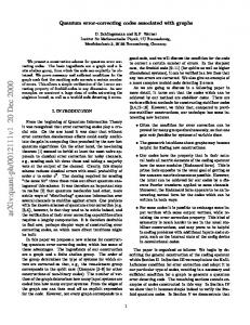
each Figure 10: configuration Instance of a has (3,6)Figure 9: Factor graph of a LDPC Thursday, October 10, 13 randomuniform factor graph, where 34 with N=20 variables 10 of factors. It was shown by Miller and Cohenand (The rate regular LDPC Codes, IEEE Trans. IT,probability 49, 2003, pp. (resp., 6)regular is the degree 2989--2992), that with high probability the rate of a randomly chosen codeaverage is very close to this of lower bound. See also page 81 in MCT (Modern Coding Theory). regular factors). code here we mean a code nodes By (resp., where all variables have degree lets say dl and all check nodes have degree, lets say dr. Thursday, October 10, 13

the n − k linear constraints implied by the parity-check matrix. There is an edge between a factor node and a variable node if that particular node participates in the constraints represented by the factor node. Since the parity matrix H is sparse, the number of edges in this factor graph only grows linearly in the length of the code. The code is then the set of all binary n-tuples that fulfill each of the n − k constraints. As an example, looking at Fig. 9 the first constraint is C1 = I(x6 ⊕ x7 ⊕ x10 ⊕ x20 = 0) where I(•) is the indicator function. The code rate, i.e., the fraction of information bits contained in the n transmitted bits, is equal to R ≥ Rdesign = #variables−#factors . In general, Rdesign is only a #variables lower bound on the actual rate since some of the constraints can be linearly dependent. But it was shown by [3], that with high probability the rate of a randomly chosen regular code is very close to this lower bound (see also [1]). A regular code one where all variables have constant degree dl and all check nodes have degree dr .

3.4

Configuration model

One possible way of generating a (dl , dr )-regular code is to define an ensemble of such codes and to create a specific instance by sampling uniformly at random from this ensemble. A canonical way of achieving this is via the so-called configuration model. In this model, associate dl “sockets” to each variable node and dr sockets to each check node. Note that there are in total ndl variable node sockets and an equal number, namely (n−k)dr check-node sockets. We get from this model a graph by picking uniformly at random a 16

⇤(x) = (x) =

1 x 4

2 4x

=

2 15

P (x) =

1 x 2

⇢(x) = =

5 2x

5 12

permutation on ndl elements and by matching up sockets according to this permutation. This ensemble is convenient for practical implementations, since it is easy to sample from, and it is also well-suited for theoretical analysis. For applications it is also important to be able to have nodes of various degrees. The corresponding ensembles of codes are called irregular ensembles. To specify such an ensembles we need to specify how many nodes there are of what degree, or equivalently, how many edges there are that connect to nodes of various degrees. One useful representation of the statistics of the degrees is in terms of a polynomial representation. For example, the polynomials corresponding to Fig. 10 are: Λ(x) = P (x) =

1 2 x + 4 1 5 x + 2

2 4 1 5 dΛ(x) 2 8 5 x + x , λ(x) = C = x + x3 + x4 4 4 dx 15 15 15 1 7 dP (x) 5 4 7 x , ρ(x) = C x + x6 (12) 2 dx 12 12

Here, Λ (P ) is the normalized distribution from the node perspective (where Λ specifies the variable node degrees and P specifies the check node degrees). The coefficient in front of xi is the fraction of nodes of degree i. The normalized derivatives of these quantities, namely λ (ρ), represent the same quantities but this time from the perspective of the edges, i.e., the represent the probabilities that a randomly chosen edge is connected to a node of a particular degree.

3.5

From Bit MAP to Belief propagation decoding

For the BEC, bit MAP decoding can be done by solving a system of linear equations, i.e, in complexity O(n3 ): one must solve Hx = 0, i.e. H x ⊕ H¯x¯ = 0, where H is submatrix of the parity-check matrix spanned by the columns corresponding to the erased components of x, i.e, x , and H¯ is the complement. Thus H x = H¯x¯ = s has to be solved to find back the missing part x . But we are interested in an algorithm that is applicable for general binary-input memoryless output-symmetric (BMS) channels, where MAP decoding is typically intractable. We therefore consider a messagepassing algorithm which is applicable also in the general case. More precisely, we consider the sum-product (also called Belief-Propagation (BP)) algorithm. This algorithm performs bit MAP decoding on codes whose factor graph is a tree, and performs well on locally tree like graphs such as the random ones (see Fig. 11) From (11) we get   X Y  p(yj |xj ) I (x ∈ C) x ˆMAP = argmax (13) i xi ∈±1

{xj :j6=i}

17

j

Bit MAP Decoder to Belief Propagation Decoder x ˆMAP = argmaxxi 2{±1} p(Xi = xi | y) i ⌘ X ⇣Y p(yj | xj ) 1{x2C} = argmaxxi 2{±1} xi

j

Figure 11: Instance of a random factor graph. The BP decoder allows to estimate the marginal or mode of each input components. Perasure

Thursday, October 10, 13

0.0 0.1 0.2 0.3 0.4 0.5 0.6 0.7 0.8 0.9 1.0

How does BP perform on the BEC?

12

For the BEC, bit MAP decoding could be done by solving a system of linear equations, i.e., in complexity n3.But we are interested in an algorithm that is applicable for general BMS channels (where MAP decoding is typically intractable). We therefore only consider a message-passing algorithm which is applicable also in the general case. More precisely, we consider the sum-product (also called belief-propagation (BP)) algorithm. This algorithm performs bit MAP decoding on codes on graphs whose factor graph is a tree.

0.0 0.1 0.2 0.3 0.4 0.5 0.6 0.7 0.8 0.9 1.0

(3, 6) ensemble

Figure 12: Performance of BP decoding over a BEC channel.


15

Here is the experiment we consider. Fix the ensemble. In the above example it is the (3, 6)-regular ensemble. This will serve as our running example. Now pick very long instances of this ensemble. Pick a random codeword and transmit over a BEC with erasure probability eps. Run the BP decoder until it no longer makes any progress. Record the error probability and average over many instances. Plot the average bit-error probability versus eps. Naturally, as eps decreases the error probability decreases. What is most interesting is that at some specific point we see a jump of the error probability from a non-zero value down to zero. This is the BP “threshold.”In the next slides, we will explain how to locate the BP threshold.

BP is a message passing algorithm that finds a fixed point to the following set of equations (here for the case of a parity check code): mi→µ (xi ) =

m ˆ µ→i (xi ) =

p(yi |xi ) Y m ˆ ν→i (xi ) zi→µ ν∈∂i \µ  X M 1 I  zˆµ→i {xj :j∈∂µ \i}

{xj :j∈∂µ \i}

(14) 



xj  ⊕ xi = 0

Y

mj→µ (xj )

{xj :j∈∂µ \i}

where ∂µ \i stands for the ensemble of variable indices of the variables that are neighbors of factor µ except i, the messages {mi→µ , m ˆ µ→i } are the socalled cavity messages (which are probability distributions, {zi→µ , zˆµ→i } are the normalization constants) from which we can infer their most probable state by maximization of the marginals {m(xi )} allowing bit MAP decoding: m(xi ) =

1 Y m ˆ ν→i (xi ) zi

(15)

ν∈∂i

What is the performances of the BP algorithm on the BEC? Here is the experiment we consider. Fix the ensemble. In the above example it is the (3, 6)-regular ensemble. Now pick very long instances of this ensemble. Pick a random codeword and transmit over a BEC with erasure probability . Run the BP decoder until convergence. Record the error probability 18

Asymptotic Analysis - Density Evolution (DE) erasure fraction at the root after iterations x(`) = ✏(y (`) )dl y (`) = 1

1

x(`

(1

1) dr 1

x(`=2) = ✏(y (`=2) )dl y (`=2) = 1

(1 (1

1

x(`=1) )dr

x(`=1) = ✏(y (`=1) )dl y (`=1) = 1

)

1

1

x(`=0) )dr

1

x(`=0) = ✏

Asymptotic Density Evolution (DE) Asymptotic AnalysisAnalysis - Density- Evolution (DE) Thursday, October 10, 13

18

Figure 13: Representation of the DE dynamics over an infinite tree, allowing So if we perform l iterations we get a sequence of erasure probabilities. This is how Gallager analysed codes. Luby et.of al. used somewhat different procedure. In of theirdecoding analysis theyat lookthe at the so-called theLDPC computation the aasymptotic probability root.

Asymptotic Analysis - Density Evolution (DE)

peeling decoder. This decoder is entirely equivalent to the BP decoder (when transmitting over the BEC). In this decoder, as long as there is a degree-one check node, we use this check node to determine one dr the1 dr 1We then follow dl remove 1 the useddcheck l 1 node as well as the determine variable. more bit and then evolution of the graph. This can be done by writing down a system of differential equations. This method is called the Wormald method ([“Differential Equations for Random Processes and Random Graphs”, N. dr 1 1 Pg. 1217-1235]). l 5, Wormald, Ann. Appl. Probability,dVol.

y

y

?

channel erasure fraction

channel erasure fraction channel erasure fraction ?

1

y ? ?

(1

1 x)

?1

(1

x)

?x)

(1

?

? ? ? ?? ? ? ? ?? y yy y y x x x xx x ? ? ? ? ? ? Figure 14:yDE iteration over a factorxand axnode. x y y one iterationone iteration one iterationone iteration ? y

of BP at variable of BP at check of BP at check of BP at variable


and average over many instances. Plot the average bit-error one iteration one iteration node node probability node node versus . Naturally, as decreases the error probability of BP at variable of BP atdecreases. check What is most interesting is that at some specific point we see a jump of the error node node probability from a non-zero value down to zero. This is the BP threshold (see Fig. 12). Thursday, October 10, 13 17

Let us the erasure probability duringprocess the decoding process a large Let us analyze how theanalyze erasurehow probability behaves during behaves the decoding for a large code.forWe do code. We do this by looking how the erasure probability behaves at each ofofthe two types of the nodes. this by looking how the erasure probability behaves at each of the two types the nodes. Consider a (d l, Consider a (dl, 3.6 Asymptotic Analysis: Density Evolution (DE) Thursday, October 10, 13 17 )-regular i.e.,node everyhas variable node hasand degree dl check and and every node dr)-regular code,dri.e., everycode, variable degree dl and every node hascheck degree dr. has degree dr. Let us analyze how the erasure probability behaves during the decoding process for a large code. We do Density evolution is a general method that allows us to analyze decoding this by looking how the erasure probability behaves at each of the two types of the nodes. Consider a (dl, At thein if therethe is an incoming which is not erasure, theisvariable node is At the variable node, ifvariable there limit is node, an incoming message whichmessage isnodes not an and erasure, thenanthe variablethen node where factors dr)-regular the code, i.e., every variablenumber node hasof degree dl and and every both checkbecome node haslarge degreebut dr. exactly determined. This is because we are transmitting over the BEC and either perfect exactly determined. This is because we are transmitting over thedoBEC and either we have their ratio remains constant. We this by looking atperfect how we thehave erasure information or we have absolutely useless On the check even if one incoming information or we have absolutely useless information. On information. the check node side, evennode if oneside, incoming At the variable node, behaves if there is at an each incoming message whichofis the not an erasure, then theavariable is probability ofoutput the two types nodes. Consider (dl , dhence )- the rnode message in erasure, check has nowhether way knowing it is 0 or message is in erasure, theischeck nodethe output hasnode no way knowing it is 0 orwhether 1 and hence the1 and exactlyregular determined. This is because we are transmitting over the dBEC and either we have perfect code, i.e., every variable node has degree and and every check node l between outgoing message an erasure as well. This input/output values outgoing message is an erasure asiswell. This input/output relation betweenrelation erasure values iserasure depicted by is depicted by information or we have absolutely useless information. On the check node side, even if one incoming has degree dr . We focus on the BEC. At the variable node, if there is an the equations above. the equations above. message is in erasure, the check node output has no way knowing whether it is 0 or 1 and hence the outgoing message is an erasure as well. This input/output relation between erasure values is depicted by that in the above equations the erasure probability entering node along or check Note that in theNote above equations the erasure probability entering a variable node aorvariable check node the node along the the equations above. edges is the edge. same This for each edge.the This simplifies the analysis considerably. various edges isvarious the same for each simplifies analysis considerably.

19

Note that in the above equations the erasure probability entering a variable node or check node along the various edges is the same for each edge. This simplifies the analysis considerably.

17

incoming message which is not an erasure, then the variable node is exactly determined. This is because we are transmitting over the BEC and either we have perfect information or we have absolutely useless information. On the check node side, even if only one incoming message is an erasure, the check node output has no way knowing whether it is 0 or 1. Denoting y (x) the probabilities that a factor (node) is undetermined, we obtain Fig. 14 giving the probabilities for a node (factor) to output no information after one iteration. So if we perform l iterations we get a sequence of erasure probabilities as shown in Fig. 13. This is how Gallager analyzed LDPC codes. Luby and. al. used a somewhat different procedure. In their analysis they look at the so-called peeling decoder. This decoder is entirely equivalent to the BP decoder (when transmitting over the BEC). In this decoder, as long as there is a degree-one check node, we use this check node to determine one more bit and then remove the used check node as well as the determined variable. We then follow the evolution of the graph. This can be done by writing down a system of differential equations. This method is called the Wormald method [2]. Note that in the density evolution approach we assume that we first fix the number of iterations and let the length of the code tend to infinity (so that there are no loops in the graph up to the desired size). We then let the number of iterations tend to infinity. In the Wormald approach on the other hand we take exactly the opposite limit. Luckily both approaches give exactly the same threshold: DE corresponds to the limit liml→∞ limn→∞ but in fact we can take the limit in any order, or jointly, and we’ll always get the same threshold: the approach is robust. The density evolution is decreasing and bounded from below and will thus converge. For large codes, the behavior of almost all of them in the ensemble is accurately predicted by DE: it is the concentration property. DE can be applied to the BEC to predict the fraction of bits that cannot be recovered by BP decoding as a function of the erasure probability (see Fig. 15). It is predicted that there exist a critical threshold ( ≈ 0.429 for the BEC) under which BP will recover the full codeword and above which it becomes impossible to recover everything. It perfectly matches the experimental threshold (Fig. 12) but the curves are different. We will understand why in the next section.

3.7

EXIT curves

Instead of plotting the x-value on the vertical axis it is often more convenient to plot the EXIT value, see Fig. 19. The EXIT value has a simple interpretation. It is the error probability of the best estimate we can do using all the internal messages at a node but without the channel observation at this bit. This is why we have y to the power dl and not dl − 1 but we do not have the factor corresponding to the channel erasure fraction. 20

Finite-Length Scaling DE for (3, 6) Ensemble x 1.0

10-1 0.8

10-2

N in

10-3

0.6

PN (R, )

erasure fraction as a function of increasing iterations for a given channel value

0.4

10-4 10

cre as

ing

-5

10-6 0.2

10-7

0.2

0.4

0.6

0.8

1.0

10-8

eps

channel quality

Figure 15: DE prediction for the fracFigure 16: The experimental curve tion of lost bits after BP decoding for getting closer to the BP threshold the BEC as a function of the erasure running Let us now apply DE for our running example. We see that up to the “BP threshold”, which for the as N increases. example is around 0.429, the erasure probability tends to zero if we let the number of iterations tend to probability. infinity. For higher values of eps the x-value tends to a non-zero value.


20


We will see soon why the EXIT value is the right quantity to plot. Rather than running the recursion we can right away find the value to which the recursion converges. This is because this final value must be a solution to the fixed-point (FP) equation x = f (, x), where f (·) denotes a recursive DE equation. The forward fixed points of DE (see Fig. 17), which follows the true decoding dynamics and with initial condition x(l=0) = are: y (l) = 1 − (1 − x(l−1) )dr −1

x

(l)

x

(l)

(16)

(l) dl −1

= (y )

= (1 − (1 − x

(17)

(l−1) dr −1 dl −1

)

)

(18)

Then, the fixed points of DE (see Fig. 18) are obtained by removing the time step index: x = (1 − (1 − x)dr −1 )dl −1 x = (1 − (1 − x)dr −1 )dl −1

(19)

Note that there are in general several values of x which satisfy the FP equation for a given , but there is always just a single value of for a given x, which is easily seen by solving for from the FP equation above. This makes it easy to plot this curve. But note also that in this picture we have additional fixed points. These fixed points are unstable and we cannot get them by running DE. The previous DE equations can be easily extended to the irregular graph case: x(l=0) = y (l) = 1 − ρ(1 − x(l−1) )

x(l) = λ(y (l) )

x(l) = λ(1 − ρ(1 − x(l−1) ))

21

28

)

=1

)

= ✏(y (`) )dl

)

0.6

0.4

1

0.2

= ✏(1

(1

x

(` 1) dr 1 dl 1

)

)

A look back ...

0.0

EXIT

All Fixed Points of DE

= ✏(1

=

1) dr 1

(1

(1 (1

0.2

0.4

0.6

0.8

1.0

eps

x

1.0

EXIT 1.0

0.8 0.8

x)dr 1 )dl x x)dr 1 )dl

(3, 6) ensemble Thursday, October 10, 13

0.0 0.1 0.2 0.3 0.4 0.5 0.6 0.7 0.8 0.9 1.0

)

x(`

(1

0.6

1 0.6

0.4

0.4

1

0.2

x versus EXIT 0.2

0.0

0.2

0.4

0.6

0.8

1.0

eps

0.0 0.1 0.2 0.3 0.4 0.5 0.6 0.7 0.8 0.9 1.0

0.0 0.0

0.2

0.4

0.6

0.8

1.0

eps

Figure 17: DE forward (stable) fixed Figure 18: All DE fixed points. points. 23

24

Let us now go back to our first experiment. We see now that we can predict where the red dots will lie. In fact, in our original experiment we cheated slightly. We printed the EXIT value and not the bit error probability. These two only differ by a factor eps. We will see soon why the EXIT value is the “right” quantity to plot.

the recursion we can right away figure out the value to which the recursion converges. final value must be a solution to the fixed-point dl 1(FP) equation x=f(eps, dl x), where f() x = ✏y EXIT = y ve DE equations. Note that there are in general several values of x which satisfies the y x, which is easily seen ven eps, but there is always just a single value of eps for a given om the FP equation above. This makes it easy to plot this curve. But note also that in e “additional” fixed points. These FPs are unstable and we cannot get them by running ee they nevertheless play an important role in the analysis.

y

y

y

y

y

y

Figure 19: The x-value versus the EXIT value. These distributions ρ() and λ() can be optimized over by finite size scaling techniques, in order to reach capacity of the channel in the large blocklength Thursday, October 10, 13 limit. For example wethe canvertical take axis a family of more the form: Instead of plotting the “x-value” on it is often convenient to plot the EXIT value. The

21

EXIT value has a simple interpretation. It is the error probability of the best1 estimate we can do using all the α “internal” messages at a node butλwithout channel observation 1− (1 − x) , ρα (x)at=this x αbit. This is why we have y to the α (x) =the power dl and not dl-1 but we do not have the factor eps corresponding to the channel erasure fraction.

and try to find the best parameter α such that the error probability decreases as fast as possible to zero below the channel capacity as N increases. In addition, the distributions must verify the matching condition: λ(1 − ρ(1 − x)) − x ≤ 0 Capacity achieving degree distributions should verify the strict conditions: λ(1 − ρ(1 − x)) −P x = 0 and have P an average degree → ∞. For instance, we can write λ(x) = i wi xi−1 with i wi = 1, wi ≥ 0. In this case λ() can be 22

inverted and the matching condition becomes: Z Z x 1 − ρ(1 − x)dx ≤ λ−1 ( )dx 0 0 Z 1− 1 1 ρ(x)dx ≤ (1 − + ) − OR OL 0 R R where OL = 0 λ(x)dx is the average node degree and OR = 0 ρ(x)dx is the average check degree. ! R 1− ρ(x)dx OL (20) →≤ 1 − R0 1 OR ρ(x)dx 0

Again, the capacity is reached only in the strict equality case. In the case where there are n nodes and m checks in the graph, the condition OL n = OL m OR m must be true, then the rate R = n−m m = 1 − n = 1 − OR = 1 − Sh OL . It implies for the where Sh is the Shannon threshold satisfying Sh = O R matching condition: ≤ Sh (1 − P (1 − Sh )) (21) where P is a polynomial that approaches 0 as OR → ∞.

3.8

Some basic facts

What we saw does not only work for the BEC but for a large class of practically relevant channels. Only for the BEC we do have a proof that these codes achieve capacity. For the general case we need to optimize numerically. So far we looked at ensembles and excluded many practical concerns. To find a particular code for a standard much care and work is needed. These are the codes which are these days included in standards. Codes are not universal but need to be constructed with a particular channel in mind.

4

Spatially Coupled Codes

So far we have discussed the simplest form of LDPC ensembles, namely ensembles that are defined by degree distributions but are otherwise completely unstructured. Such ensembles can have good performance (e.g., we have seen that for the BEC they can achieve capacity) but “real” codes typically have additional structure which allows to optimize various performance metrics. We will now discuss one such structure which is called spatial coupling. As we will see, this structure will allow us to construct capacity-achieving ensembles for a much broader class of channels and it is nicely grounded in basic facts from statistical physics.

23

Figure 20: In the protograph construction we start with a single “protograph.” (see e.g., the left-most graph on the left side). We then “lift” this protograph to a larger graph by taking M copies (in our specific case M = 5. Finally , we connect the various copies by taking “like” edges (which we call an edge bundle and by permuting the edges in the edge bundle via a permutation picked uniformly at random. One particular edge bundle is shown on the left by dotted lines and the result of the permutation is shown on the right.

4.1

Protographs

There are many ways of describing LDPC ensembles and many flavors of such ensembles. One particularly useful way of describing an ensemble is in terms of so-called protographs. This language will be useful when describing the more complex case of spatially-coupled ensembles. Protographs were introduced by Thorpe [5]. They give a convenient and compact way of specifying ensembles and the additional structure they impose is useful in practice. The creation of a “real” graph from protographs is illustrated in Fig.20. For simplicity, M = 5 copies are introduced in Fig. 20, but M is typically in the order of hundreds or thousands. The edges denoted by dashed lines in Fig. 20 are “edge bundles.” Such an edge bundle is a set of “like” edges that connect the same variable node and the same check node in each protograph. In a protograph we connect the M copies by permuting the edges in each edge bundle by means of a permutation chosen uniformly at random as shown in right of Fig. 20. Strictly speaking, the ensemble generated in this way is different from the ensemble generated by the configuration model, but these models are asymptotically equivalent in the sense that density evolution as discussed before gives the correct asymptotic predictions in both cases.

4.2

Construction of Spatially Coupled Codes

Let us now introduced spatially coupled ensembles. There are as many flavors and variations of spatially coupled codes as there are for uncoupled codes. The exact version we consider here is not so important since they all 24

Figure 21: Spatially coupled codes (right) constructed from a set of (3, 6) protographs (left). behave more or less the same. Hence, let us consider two variants that are easy to describe and are typical. The first is a protograph-based construction whereas the second one is purely random. 4.2.1

Protograph construction

In the protograph construction, we start by taking a certain number of like protographs and placing them next to each other on a line as shown on the left in Fig. 21. We then “connect” neighboring copies in a regular fashion as shown on the right in the figure. This gives us a protograph which has a spatial structure, explaining the origin of the name “spatially coupled.” Note that towards the middle of the chain the degree structure of the graph is exactly the same as the degree structure of the protograph we started with. Only towards the boundary, due to boundary effects do we have a different degree structure. Note that a variable node in the picture is connected to 3 different positions. We therefore say that the “connection width” is 3 and we write w = 3. At the boundaries, the code has more available information in the sense that the number of edges are less than the middle part as shown in Fig. 21. As we will see, this boundary condition plays a crucial role. Note that the right picture in Fig. 21 is not the graph (code) itself yet but just a protograph representing the code. As mentioned in Sec. 4.1, to generate the real code from a given protograph, we need to “lift” the graph M times and then randomly permute edges in the same edge bundle. Note: Coupled codes constructed in this way from protograph show an excellent performance and are ideally suited for implementation by virtue of the additional structure. But they are more difficult to analyze than the random construction which we discuss below. 4.2.2

Random construction

In the random construction we have the same spatial structure for the nodes but edges connecting neighbors a placed in a more random fashion. More 25

w

L Figure 22: Random construction of spatially coupled codes. Edges are defined randomly in the shaded area. precisely, we randomly connect check nodes and variable nodes within a window of size w as shown in Fig. 22. Again, we ensure that the degree distribution away from the boundary is equal to the degree distribution of the original code. Note that when w = L, then in fact we impose no spatial constraints on the connectivity, and we recover the standard uncoupled LDPC ensemble. This randomly constructed coupled ensemble performs slightly worse in terms of its finite-length performance but it is easier to analyze since it has fewer parameters.

4.3

Why spatial coupling

Before we proceed with the theoretical analysis of the spatially coupled ensembles, let us quickly show that spatially coupled ensembles behave quite differently from uncoupled ensembles when we let the degrees tend to infinity. Since the local degree distribution is the same, this will show that the spatial structure indeed leads to some interesting behavior. 4.3.1

Degree dependence of the uncoupled ensembles

The two pictures in Fig. 23 show the fixed points of density evolution for the uncoupled case for (a) the (3, 6) LDPC ensemble and (b) the (100, 200) LDPC ensemble. Note that both have a rate of one-half. The solid and dashed line represent stable and unstable fixed points, respectively, and the vertical lines represent the BP threshold; for (a) we have BP = 0.42944 and for (b) we have BP = 0.0372964. As shown we can see from Fig. 23, and as one can show analytically, as we increase the degree the BP threshold decreases and it reaches 0 when the degree tends to infinity. Is this decrease of the threshold due to the fact that the associated code gets worse as the degrees become larger or is it the fault of the (suboptimal) BP decoder? A closer look reveals that the code itself in fact gets better as the degree increases. But the decoder becomes more and more suboptimal.

26

(a)

1

0.8

x*

0.6 0.4 0.2 0

(b)

0

0.2

0.4

ε

0.6

0.8

1

0

0.2

0.4

ε

0.6

0.8

1

1

0.8

x*

0.6 0.4 0.2 0

Figure 23: Fixed points of uncoupled (a) (3, 6) code and (b) (100, 200) code. The vertical lines represent threshold (a) BP ' 0.42944 and (b) BP ' 0.0372964.

27

4.3.2

Spatial coupling might help

Let us now repeat the above experiment with spatially coupled ensembles. We will see that they behave very differently. Consider a coupled ensemble constructed via the protograph approach. To make the argument particularly simple, assume that all the edges between factor nodes and variables nodes are in fact double edges, as shown in Fig. 24. E.g., the protograph shown in this figure therefore represents an (4, 8)-regular ensemble. Consider now the decoder procedure. We want to show that the BP threshold does not tend to zero for such an ensemble even if we increase the degrees and let them tend to infinity. To show this note that we can get a lower bound on the decoding threshold by “weakening” the decoder. We weaken the decoder in the following way. Instead of allowing the decoder to use all available information, assume that when we decode the bits in the first position we are not allowed to use the information we received in any of the positions to the right. This means that for the given example we concentrate only on the double edges connected to a factor node (denoted by solid lines in Fig. 24) and ignore other edges (denoted by dashed lines). Note that if we concentrate on the bits in the left-most position this means that we are decoding a (2, 4)-regular code, which is also known as “cycle code.” The BP threshold of such a code is known and e.g. for the BEC it is equal to BP = 1/3. Therefore, we know that we can decode the left-most bits using the BP decoder if we transmit over a BEC with erasure probability not exceeding 1/3. Now assume that these positions are known. We can then remove (the effect of) these bits from the graph. But if we do so, what is left looks again exactly like the original situation except that now the chain is shorter by one. We can therefore recurse our argument. In summary, we have just argue that the BP threshold of this chain is at least one-third. The punch line is now the following. Exactly the same argument holds if we increase the degrees and look at the spatially coupled (2k, 4k)-regular ensemble, regardless of the value of k. Therefore, the BP threshold does not tend to zero for coupled ensembles even if we let the degrees tend to infinity. This argument only shows that the threshold is lower bounded by a constant and it does not permit to determine the actual threshold. In fact, we will shortly see that the actual threshold improves as the degree gets larger.

5

Density Evolution for Coupled Codes

Let us now get to the analysis of coupled ensembles using the same method, namely density evolution, which we used in the uncoupled case. In the uncoupled case, the variable x, which represents the erasure fraction along an outgoing edge from the variable node, is a scalar and density 28

Figure 24: A coupled (2, 4) ensembles with double edges.

xi

ε

yi

… yi

… yi+w-1

xi-w+1

xi

Figure 25: Density evolution in spatially coupling code with width w. evolution tracks the evolution of this scalar as a function of the iteration number. For the coupled case the state is a vector, since variables at different positions will not experience the same “environment.” Recall that at the boundary we have a slightly different degree distribution and the decoder problem is easier there. As we will see, the decoder will be able to decode at the boundary first and this progress will then propagate towards the interior of the code along a “decoding wave.” Due to this lack of “homogeneity” along the spatial dimension we need a vector x to describe the state, where xi describes the erasure probability at position i (= 1, · · · , L). Recall that we know the values at the boundary, and hence the erasure probability at the boundary is 0. In the randomly constructed code, each edge can be connected to positions in a certain range. More precisely, consider Fig. 25: variable nodes assigned {xi } are always connected to position “to the right” and check nodes assigned {yi } are always connected to variable nodes “on the left”. 29

We therefore need to average over the incoming messages from this range, and the density evolution equations for the coupled ensemble are given by 1 w−1 dl −1 X xi = yi+j w

(22)

yi = 1 − 1 −

(23)

j=0

w−1 dr −1 1 X xi−k , w k=0

where i = 1, · · · , L. Note that there is an xi and an yi value for each position of the chain and the equations for these values are coupled through the averaging operations. Combining equations (22) and (23) and adding an index for the iteration number we get w−1 w−1 1 X 1 X (l−1) dr −1 dl −1 (l) xi+j−k ) . xi = 1 − (1 − w w j=0

(24)

k=0

To simplify our notation, and also to abstract from the specific case we are considering, let us define the functions {fi (·)} and g(·), w−1 w−1 dr −1 dl −1 1 X 1 X xi−k , g({xi∈I(i) }) = 1 − fi = 1 − fi+j , w w

(25)

j=0

k=0

where I(i) denotes set of indices connected to i. In this way we get simple expressions, like xi = g({xi∈I(i) }).

(26)

We call a vector x = {xi } (i = 1, · · · , L) whose components are the erasure fractions at the various indices a constellation. At all the indices outside the constellation, i < 1 and i > L, we assume that the corresponding xi values are 0, i.e., we have perfect knowledge. A constellation x which when inserted into the DE equations results in x is called a fixed point of DE equation. In Fig. 26, the -dependence of the time evolution of the DE equation for the coupled ensemble, according to equation (24), is shown. Picture (a) corresponds to = 0.3, (b) corresponds to = 0.48, and (c) is for = 0.6. Note that for < BP ' 0.4294, DE proceeds in essentially exactly the same way as for the uncoupled case if we look at the xi values in the center of the chain. At the boundary we see somewhat better values due to the boundary condition. And as expected, the DE is able to drive the erasure fraction in each section to zero and BP is successful. At = 0.48, which is considerably larger than the BP threshold BP = 0.4294 of the uncoupled ensemble (and close to the optimal threshold of 0.5 30

1

1

(b)

(a)

0.6

0.6

xi

0.8

xi

0.8

0.4

0.4

0.2

0.2 0

0 0

20

40

60

i

80

0

100

20

40

i

60

80

100

1

(c) 0.8

xi

0.6 0.4 0.2 0 0

20

40

i

60

80

100

Figure 26: Time evolution of {xi } by DE equation for the (3, 6) coupled code at (a) = 0.3, (b) = 0.48, and (c) = 0.6. The length is L = 100 and width is w = 20. The constellations evolve in the order of solid line → dashed line → dotted line → dashed-dotted line.

31

of the best code and decoding algorithm), a small “wave front” is formed at both boundaries after a few iterations due to the fact that at the boundaries more knowledge is available, see Fig. 26 (b). These wave fronts move towards the center of the coupled code at a constant speed and by doing so decrease the value of xi for i located in the central part of the coupled code until the whole constellation is decoded. This is the interesting new phenomenon that happens due to the spatial structure. In other words, due to the spatial structure, the wave front can smoothly connect the desired fixed point of xi = 0 to the undesired fixed point that is found by the BP decoder of the uncoupled system and at a constant speed the undesired fixed point is guided towards the desired one until decoding is accomplished. As we increase the parameter up to a critical threshold, call it Area , the speed of the wave is linearly decreased and it reaches the value zero at Area . At above Area , we get a non-trivial fixed point of DE and decoding is no longer successful. In the middle of the chain the xi values are exactly as large as they would be for the same value in the uncoupled case. Only at the boundary do we get somewhat better values because of the boundary condition.

5.1

Summary

In the following sections, we will see that spatially coupled ensembles can be decoded up to Area and this value is essentially equal to MAP of the underlying ensemble. This phenomenon is called threshold saturation. In order to exactly achieve MAP , we have to let the chain length L tend to infinity (this makes decoding harder) and the interaction width w tend to infinity as well (with w 0, must be of order O(w). Note that the two stable fixed points of DE for the uncoupled system, namely 0 and x∗ , are essentially the lower and upper bounds on x and that x should smoothly interpolate between them. For simplicity, we consider DE for one-side constellations (x−L , · · · , x0 ) ∈ [0, 1]L+1 as shown in the right of Fig. 28, where L is the length of the chain and x−L < · · · < x0 . The DE equation for one-side constellations is obtained from the usual coupled DE equation eq. (24) by setting xi = 0 for i < −L and xi = x0 for i > 0. We define the average value (entropy) of the one-side constellation as x=

0 X 1 xi . L+1

(27)

i=−L

We can establish the existence of the fixed point with the desired properties by the use of Schauder’s fixed point theorem, which states that any continuous mapping f from a convex compact subset S of a Euclidean space to S itself has a fixed point. In fact, when applying the fixed point theorem we do not fix the parameter , but this parameter is part of fixed point itself. Therefore, as a consequence of Schauder’s fixed point theorem, after some proper definition of the fixed point equation we are guaranteed the existence of a constellation x∗ with the desired properties which is a fixed point for some channel parameter ∗ . Although one can establish a priori bounds on 35

(a)

1

γ = 0.85 γ = 0.63 γ = 0.4 γ = 0.3

0.8

xi

0.6 0.4 0.2 0 -6

-5

-4

-3

-2

-1

0

i (b)

1

γ = 0.85

0.9 0.8

γ = 0.63

EXIT

0.7 0.6 0.5 0.4

γ = 0.4

0.3 0.2

γ = 0.3

0.1

εArea

0 0

0.2

0.4

0.6

0.8

1

ε

Figure 29: (a) Examples of interpolated family for (3, 6) coupled code with L = 6 and w = 2 and (b) corresponding EXIT curve. Dashed line denotes EXIT curve of uncoupled case. the range of ∗ , its exact value is not known. This is the point of the next step in the proof. 6.1.3

Saturation

Next, we show that when we have the special fixed point, its channel parameter must be very close to Area . The basic idea is very simple. Recall our discussion of the EXIT curve for the uncoupled system. In this case we mentioned that the area enclosed “within” this EXIT curve is equal to the rate of the code. For the uncoupled case this was the result of a simple explicit computation since the EXIT curve was known in parametric form and the integration can be carried out without problems. But there exists also a more conceptual proof which does not rely on explicit calculations and which shows that any time you have a smooth EXIT curve the area it encloses must be equal to the rate of the code. Why is this true? It turns 36

out that the EXIT curve can be interpreted as the derivative of an entropy term with respect to the channel parameter and so when we integrate, by the fundamental theorem of calculus, the area is just the difference of this entropy term at the two end points. This difference can be determined explicitly and it happens to be equal to the rate of the code. More is true, assume that instead of have a real EXIT curve, where we recall that each point corresponds to a fixed point of DE) we have a smooth curve where every point corresponds to an “approximate” fixed point of density evolution. Here, “approximate” means that the difference of the point and the point we get after one iteration is small in the appropriate metric. In this case the same conceptual argument tells us that the area enclosed by this curve is “close” to the rate of the code, where the measure of “closeness” is related to how close the points are to being fixed points. The idea is hence the following. Given the special fixed (∗ , x∗ ) we will construct from it a whole family of approximate fixed points so that this family gives rise to an approximate EXIT curve. The shape of the approximate EXIT curve is the one shown as a solid curve in Fig. 29(b). In particular, the sharp vertical drop happens exactly at the parameter ∗ and the whole EXIT curve will look just like the curve we get from the Maxwell construction. Applying then the fact that the integral must be equal to the rate of the code will tell us that the sharp vertical drop must happen exactly at the area threshold. But how can we construct from this single special fixed point a whole family? Rather than discussing the whole construction let us only discuss the most interesting part, namely the part corresponding to the sharp vertical drop. Recall that one of the conditions on the special fixed point was that in the “middle” the fixed point was essentially flat and had a value essentially equal to what the uncoupled ensemble would have for this channel parameter. Further, towards the boundary the boundary the values had to be essentially equal to 0. This means that we insert any number of further sections in the middle with the appropriate value or any number of further sections at the boundary with the value 0 and we will still have an appropriate fixed point. All of them will be appropriate fixed points corresponding to the same channel value but their average value will depend on how wide we make the middle part. By changing this width we get points on the vertical line. Since the width can only be changed in discrete steps but we need a continuous curve we also need to interpolate the discrete steps. In addition, in order to get the points on the top horizontal portion of the EXIT curve we also need to interpolate. This is shown in Fig. 29(a). 6.1.4

Convergence

We now get to the last part of the argument. By now we have established that such a special fixed point can only exist if its channel parameter is very 37

xi Special fixed point

ξ** ξ* i 0

L

Figure 30: Assumed fixed point ξ ∗ at BP < < Area , special fixed point, and a fixed point ξ ∗∗ obtained by applying DE for the special fixed point at . close to the area threshold. We will now argue that if we start DE with a channel value below this area threshold that it must converge to the all-zero constellation. To see this, we consider the following experiment. We apply DE at BP < < Area to a constellation of size length L whose initial condition is the all-one vector inside the constellation and 0 outside. DE produces a sequence of monotonically decreasing (point-wise) constellations which are bounded by 0 (again point-wise) from below. We denoted the fixed point by ξ ∗ and assume that ξ ∗ is non-trivial, i.e., is not all-zero as shown in Fig. 30. It is clear that at each point in the constellation, the value of the fixed point is no larger than the fixed point we would get for the uncoupled case at since at the boundary the decoder has access to additional information. Now let us compare this fixed point to our special fixed where we pick the length for this special fixed point sufficiently large so that this special fixed point dominates ξ ∗ everywhere point-wise. Note that ξ ∗ is a fixed point for the parameter but the special fixed point is for the parameter Area and < Area . So if we now apply DE to the special fixed point but with the parameter then the special fixed point must be decreasing strictly point-wise and it must in fact converge to the all-zero constellation since otherwise we would get another non-trivial fixed point which would again fulfill all the requirements of a special fixed point (this needs some arguments to prove this) and we know that the only channel parameter for which such a special fixed point exists is very close to Area , a contradiction. But since our putative fixed point ξ ∗ is dominated by our special fixed point and the special fixed point collapses to the all-zero constellation it must in fact be true that ξ ∗ is also the all-zero constellation.

38

1

1

(a)

0.6

0.6

x

0.8

x

0.8

0.4

0.4

0.2

0.2

(b)

0

0 0

0.2

0.4

0.6

y 1

0.8

0

1

0.2

0.4

y

0.6

0.8

1

(c)

0.8

x

0.6 0.4 0.2 0 0

0.2

0.4

y

0.6

0.8

1

Figure 31: EXIT charts of (3, 6) uncoupled LDPC for (a) = 0.35, (b) = BP ' 0.4294, and (c) = 0.5.

6.2 6.2.1

Proof by EXIT charts EXIT charts

EXIT charts were introduced by S. ten Brink as a convenient way of visualizing DE [9]. For transmission over the BEC, the EXIT chart method is equivalent to DE. EXIT charts and EXIT curves which we have already introduced are quite different despite their similar name. The reason both objects have the word “EXIT” in there is that in both cases we measure the same thing (namely if the “other” bits in a code are able to determine the bit we are considering via the code constraints), but for EXIT charts we make local measurements, whereas for EXIT curves we measure the performance of the whole code. An EXIT chart consists of two curves. One curve corresponds to the message-passing rules at the variable nodes and the other one to the message passing rules at the check nodes. In addition, it is customary, and it is convenient, that we plot one curve with its input on horizontal axis and its output on the vertical axis and the other curve is the plot with its output on horizontal axis and its input on the vertical axis. Fig. 31 shows the EXIT charts of uncoupled (dl , dr )-LDPC for dl = 3 and dr = 6 at three channel

39

parameters, where two curves are given by x = y dl −1

(28) dr −1

y = 1 − (1 − x)

.

(29)

On this EXIT chart, the DE trajectory can be regarded as a staircase pattern bound by these two curves. The DE points converge to zero if and only if the two curves do not cross (Fig. 31(a)). The threshold for the uncoupled case is given by the channel parameter so that the two EXIT curves just touch but do not cross (Fig. 31(b)). At > BP , two curves touch at three points (Fig. 31(c)). 6.2.2

Proof by EXIT charts for coupled code

In the coupled systems, the criterion of the threshold, namely that the two curves may touch but are not allowed to cross, is relaxed. To determine the threshold for the couple system, the two EXIT curves are now allowed to cross but not by too much, and indeed, the threshold relates to a balance of areas enclosed by two curves. One can show that the condition for the threshold is exactly the same as the matching of areas condition which we have seen in the Maxwell construction. The first step of the proof consists of considering an appropriately chosen continuous version of the constellation. For the random coupled ensemble, we have introduced the window w, within which the random connections are generated. This discrete system is difficult to analyze. Instead, one can consider the limit when w goes to infinity, of course, the length of the chain has to go to infinity as well. If we increase the length w and scale the length of the code by the same proportion then in the limit we can treat the constellation as a continuous curve rather than a set of spikes. DE equation for this continuous constellation is given by integrating over a window instead of taking discrete sums. The next step is to analyze this continuous system. It is convenient to think of systems of infinite length, i.e., the horizontal axis extends from −∞ to −∞. Further, instead of consider a two-sides constellation, we consider a one-sided constellation, i.e., we only focus on the “left” part of the constellation from −∞ to 0. For the continuous system, it is proved that one has three different scenarios depending on the balance of the areas in the EXIT chart picture of the uncoupled system. We omit here the trivial case where the curves do not overlap at all since in this case it is easy to show that we will decode. Consider first the scenario where the channel parameter is below Area , but above the BP of the uncoupled ensemble (Fig.32(a)). In this case, the curves do overlap but only little and the area on the left (green) is larger than the area on the right (yellow). One can show that there does not exist 40

1 0.9

1

(a)

0.9

0.8

0.8

0.7

0.7

0.6

0.6

0.5

0.5

0.4

0.4

0.3

0.3

0.2

0.2

0.1

0.1

0

0.1 0.2 0.3 0.4 0.5 0.6 0.7 0.8 0.9 1 0.9

0

1

(b)

0.1 0.2 0.3 0.4 0.5 0.6 0.7 0.8 0.9

1

(c)

0.8 0.7 0.6 0.5 0.4 0.3 0.2 0.1 0

0.1 0.2 0.3 0.4 0.5 0.6 0.7 0.8 0.9

1

Figure 32: EXIT charts of a coupled system for (a) < Area , (b) = Area and (c) > Area . These figures are quoted from lecture materials [10].

41

0.05

ε = 0.35 ε = 0.42944 0.04 ε = 0.48818 ε = 0.52

U(x,ε)

0.03 0.02 0.01 0 -0.01 0

0.1

0.2

0.3

0.4

0.5

x

0.6

0.7

0.8

0.9

1

Figure 33: Potential function of (3, 6) uncoupled LDPC. a fixed point of DE but there exists a one-sided constellation x. If we apply DE to this constellation, we get the same x but the position is shifted to the right. Given that our one-sided constellation represents the left part of an actual constellation, saying that the wave is propagating to the right means that the decoder is working and in each step decodes a further part of the constellation. The shift which we see in each iteration corresponds to the decoding speed and so tells us how many iterations we will need. To summarize, below the area threshold we get a decoding wave which moves to the right, that means the working of the decoder. Assume next that the areas are exactly in balance, this means that we are transmitting exactly at Area (Fig. 32(b)). In this case one can prove that the continuous version of DE has a fixed point. This fixed point can be regarded as a stationary wave or a wave with zero speed. Finally, consider the case where we are transmitting above Area (Fig. 32(c)). The curves overlap so much so that the area on the left is smaller than the area on the right. For this case one can then show that there does not exist a non-trivial fixed point but only a continuous constellation x, so that after one round of DE we get the same constellation back but shifted to the left. This means that the decoder does not work. In a final step one needs to reconnect the continuous system to the actual discrete system and show that if the w is not too small then the behavior of the discrete system is well predicted by the behavior of the continuous system [11].

42

6.3 6.3.1

Proof by Potential Functions Potential Functions

The potential function for uncoupled LDPC code is defined as Z x (z − f (g(z); ))g 0 (z)dz U (x, ) = 0

= g(x) − G(x) − F (g(x); ),

(30)

Rg where f (g(z);R) = λ(1 − ρ(1 − z)), g(z) = 1 − ρ(1 − z), F (x; ) = 0 (z; )dz, x and G(x) = 0 g(z)dz. The functions λ(·) and ρ(·) are node-perspective degree distributions. The potential function corresponds to Bethe free energy. Fig. 33 shows the x-dependence of the potential function for (3, 6) uncoupled LDPC, where λ(x) = x2 and ρ(x) = x5 . When is smaller than BP ' 0.42944, the potential function is an increasing function for all x ≥ 0. At = BP , the potential function have zero gradient at a certain x, and at > BP , a local minimum appears and its value touches to the line 0 at Area ' 0.48818. This means that the state x = 0 is always exists as the unique solution when < BP . At > BP , another locally stable solution appears at x > 0, although the solution x = 0 is the globally stable state. At > Area , the solution x = 0 is no longer a globally stable solution. In physical terminology, area threshold and BP threshold correspond to the first transition point and spinodal point, respectively. 6.3.2

Potential Functions for coupled system

The potential function of the coupled system, which is defined for a vector constellation x, is introduced in analogy to the uncoupled system. We consider the potential function for one-sided constellation; xi = 0 when i is not in [−L, i0 ] and the value of xi increases with i up to i0 = b(w − 1)/2c, given by [12]; Z U (x; ) = g 0 (z)(z − AT f (Ag(z; ))) · dz C

= g(x)T x − G(x) − F (Ag(x); ),

(31)

where g 0 (x) = P diag([g 0 (xi )]), [f (x; )]i =R f (xi ; ), [g(x)]i P = g(xi ), G(x) = R g(z) · dz = G(x ) and F (x; ) = f (z; ) · dz = i i i F (xi ; ). The C C

43

matrix A is a (L + 3w + i0 + 1) × (L + 3w + i0 + 1) matrix given by   1 1 ··· 1 0 ··· 0  .  ..  0 1 . ..  1 ··· 1    .. . .  .. .. .. ..   . . . . . . 0  1  1 1 ··· 1  A =  0 ··· 0 , w . .. 1   0 0 ··· 0  1    ..   0 0 ··· 0 0 1 .  0 0 ··· 0 0 0 1

(32)

which gives matrix notation of the DE equation eq.(24). We set Kf,g = ||g 0 ||∞ +||g 0 ||2∞ ||f 0 ||∞ +||g 00 ||∞ , where ||h||∞ = supx∈[0,1] |h(x)| for functions h : [0, 1] → R [12]. Using the potential function, it can be shown that when < Area and w > Kf,g /∆E(), coupled potential of a non-zero vector decreases by the shifting. It implies that the value of constellation must be reduced by recursion, and the fixed point is the zero vector. The outline is as follows. Let us assume that x 6= 0 is the unique fixed point of the one-sided DE equation. We introduce a right-shifted constellation from x as Sx, where [Sx]1 = 0 and [Sx]i = xi−1 for i ≥ 2. The difference of the potential functions between Sx and x is given by U (Sx; ) − U (x; ) = −U (xi0 ; ).

(33)

Meanwhile, Taylor expansion of U (Sx; ) around x gives Kf,g w < −U (xi0 ; ) + ∆E() ≤ 0,

U 0 (x; ) · (Sx − x) ≤ (U (Sx; ) − U (x; )) +

(34)

where we exploit w > Kf,g /∆E(). When all components of Sx − x are non-positive, at least one component of U 0 (x; ) should be positive to satisfy eq.(34). The derivative is given by [U 0 (x; )]i = g 0 (xi )[x − AT f (Ag(x; ))]i and g 0 (x) ≥ 0, and hence [AT f (Ag(x; ))] < xi should hold. It means that one more iteration reduce the value of the i-th component. This gives a contradiction and means that the fixed point of the one-sided constellation is only x = 0 at w > Kf,g / ∆E().

6.4

Summary

We have shown three proofs of the threshold saturation phenomena. These three different criteria each have their own advantage. The first proof makes not only determines the threshold of the coupled system but makes it clear

44

that this is equal to the MAP threshold. The EXIT chart approach is convenient for people who are already familiar to EXIT charts for uncoupled systems and this criterion is very easy to apply. Finally, the potential function approach leads to the currently simplest proof of the threshold saturation phenomenon. In more detail, let us summarize some of the main points of these three proofs. In the proof by the Maxwell construction, at the area threshold, a special fixed point exists, which has long tails, quick transition, and large flat part. This special fixed point cannot exist below the area threshold (and neither can it exists at larger channel parameters). This proof has a connections to problems in statistical physics and the picture is exactly the same if we consider transmission over general BMS channels, although the proofs are more complicated. Further, it strongly suggests that the area threshold is also the MAP threshold of the underlying ensemble. Indeed, that this is true has recently been shown [13]. In the EXIT chart approach, at the area threshold, a stationary wave exists. Below the area threshold, a propagating wave, traveling at a constant speed, shows that decoding will be successful. This approach, in particular, EXIT charts and the matching condition are frequently used to analyze systems which have a one-dimensional state and they are often use to approximately model more general systems (e.g., Gaussian approximation). For any such system, if we replace the matching condition with the area balance condition then we get the equivalent criterion for coupled systems. If the original state is one dimensional then this criterion is exact, otherwise it is an approximation in the same way as the matching condition for EXIT charts is an approximation for uncoupled systems. Finally, in the potential function approach, at the area threshold, the potential function has zero gradient. Below the area threshold, potential energy is strictly decreasing implying convergence to perfect decoding. It leads to the currently simplest known proof for one dimensional systems. It can be extended to systems whose state is no longer a scalar but a vector and even to infinite-dimensional systems, e.g., general BMS channels.

References [1] Richardson T. & Urbanke R, Modern Coding Theory, (Cambridge University Press, 2009). [2] Wormald N. Differential equations for random processes and random graphs, Annals of Applied Probability, 5, 1218–1235 (1995). [3] Miller G. & Cohen G. The rate of regular LDPC codes, Information Theory, Proc. IEEE International Symposium on, 89 (2003).

45

[4] Arikan E. Channel polarization: A method for constructing capacityachieving codes for symmetric binary-input memoryless channels, Information Theory, IEEE Transactions on, 55, (7), 3051–3073 (2009). [5] Thorpe J. Low-Density Parity-Check (LDPC) Codes Constructed from Protographs, IPN Progress Report, 42-154, 1–7 (2003). [6] Kudekar S., Richardsony T. & Urbanke R. Threshold Saturation via Spatial Coupling: Why Convolutional LDPC Ensembles Perform so well over the BEC, Information Theory, IEEE Transactions on, 57, (2), 803–834 (2011). [7] Kudekar S., Méasson C., Richardson T. & Urbanke R. Threshold Saturation on BMS Channels via Spatial Coupling, Proc. 6th International Symposium on Turbo Codes and Iterative Information Processing (ISTC), 309–313 (2010). [8] Méasson C., Montanari A. & Urbanke R. Maxwell Construction: The Hidden Bridge between Iterative and Maximum a Posteriori Decoding, arXiv preprint arXiv:cs/0506083 (2005). [9] ten Brink S. Convergence of Iterative Decoding, Electronics Letters, 35, (10), 806–808 (1999). [10] EPFL-IPG, http://ipg.epfl.ch/doku.php?id=en:publications: scc_tutorial (2013). [11] Kudekar S., Richardson T. & Urbanke R. Wave-Like Solutions of General One-Dimensional Spatially Coupled Systems, arXiv preprint arXiv:1208.5273 (2012). [12] Yedla A., Jian Y., Nguyen P. S., & Pfister H. D. A Simple Proof of Threshold Saturation for Coupled Scalar Recursions, Proc. 7th International Symposium on Turbo Codes and Iterative Information Processing (ISTC), 51–55, (2012). [13] Giurgiu A., Macris N. & Urbanke R. Spatial Coupling as a Proof Technique, arXiv preprint arXiv:1301.5676 (2013). [14] Hassani S. H., Alishahi K. & Urbanke R. Finite-Length Scaling of Polar Codes, arXiv preprint arXiv:1304.4778 (2013). [15] Strassen V. Asymptotische Abschaetzungen in Shannon Informationstheorien, Trans. 3d Prague Conf. Inf. Theory, 689–732 (1962). [16] Polyanskiy Y., Poor H.V. & Verdu S. Channel Coding Rate in the Finite Blocklength Regime, Information Theory, IEEE Transactions on, 56, (5), 2307–2359 (2010).

46