ERROR ESTIMATES FOR A TIME DISCRETIZATION METHOD FOR

ERROR ESTIMATES FOR A TIME DISCRETIZATION METHOD FOR THE RICHARDS’ EQUATION IULIU SORIN POP§ Abstract. We present a numerical analysis of an implicit time discretization method applied to Richards’ equation. Written in its saturation-based form, this nonlinear parabolic equation models water flow into unsaturated porous media. Depending on the soil parameters, the diffusion coefficient may vanish or explode, leading to degeneracy in the original parabolic equation. The numerical approach is based on an implicit Euler time discretization scheme and includes a regularization step, combined with the Kirchhoff transform. Convergence is shown by obtaining error estimates in terms of the time step and of the regularization parameter.

1. Physical motivation Richards’ equation (see, for example, [4]) is a popular model for saturated-unsaturated flow in porous media. Assuming a constant air pressure in the medium, two physical quantities are unknown in this equation, the saturation and the pressure in the fluid phase. Depending on the regime of flow (unsaturated, or completely saturated), one has to decide which of the two is the primary unknown. This leads to three main forms of the Richards’ equation, saturation based, pressure based, or mixed. Here we are interested in the unsaturated case. If the porous medium is wetted by a liquid (water) of density ρ, Darcy law relates the flow velocity q to the permeability of the medium K and the pressure inside the fluid Ψ, (1.1)

q = −K∇(Ψ + z),

with z denoting the vertical coordinate in the medium. The continuity condition ∂t (ρΦ) + ∇ · (ρq) = 0 combined with Darcy law (1.1) leads to Richards’ equation (1.2)

∂t (ρΦ) − ∇ · (ρK∇(Ψ + z)) = 0.

Assuming the wetting phase has a constant density ρ, the equation above contains two unknowns, namely the saturation Φ and the pressure Ψ. Moreover, in case the medium is not completely saturated, the permeability K depends on the saturation of the medium. Based on experimental results, different retention curves relating the permeability and the pressure to the saturation have been proposed in the literature. Taking into account these relationships we can re-formulate equation (1.2) in terms of the dimensionless fluid Key words and phrases. Unsaturated porous media, Richards’ equation, degenerate parabolic problem, regularization, implicit scheme, error estimates. § Department of Mathematics and Computer Science, Technical University Eindhoven, P. O. Box 513, 5600 MB Eindhoven, The Netherlands ([email protected]). 1

2

I. S. Pop

Φ − Φr , where Φr (the residual fluid Φs − Φr content) and Φs (the fluid content at saturation) are parameters of the medium which can be obtained experimentally. In this paper we tacitly adopt the retention curves proposed by van Genuchten ([10]) µ ¶m 1 (1.3) u= , 1 + (c|Ψ|)n content (reduced saturation) u, defined by u =

where c > 0, m ∈ (0, 1) and n > 1 are again parameters of the porous medium. As 1 suggested in [10], we assume here the relation n = 1−m holds. One possibility for predicting the hydraulic conductivity knowing the saturation and the pressure inside the fluid is given by Mualem ([19]) ·Z u ¸2 Z 1 1 1 1 K = Ks Kr (u) = Ks u 2 dv dv , 0 Ψ(v) 0 Ψ(v)

/

where Ks stands for the absolute permeability of the medium (possibly depending also on on the position inside the medium, but not on the fluid saturation), and Kr for the relative permeability (depending on the saturation). Recalling (1.3), the dependence of the permeability on the reduced saturation can be given explicitly h ³ ´m i2 1 1 (1.4) K(u) = Ks u 2 1 − 1 − u m . Richards’ equation (1.2) can be rewritten now in terms of the reduced saturation µ ¶ K(u) (1.5) ∂t u − ∇ · D(u)∇u + ∇z = 0, Φs − Φr with the moisture diffusivity D(u) defined by ∂Ψ (1 − m)Ks 1 1 D(u) = −K(u) = u2−m ∂Φ αm(Φs − Φr )

·³ 1−u

1 m

´−m

³ + 1−u

1 m

´m

¸ −2 .

The equation above is nonlinear parabolic. Moreover, for u = 0 (fluid at residual saturation) the diffusivity D vanishes, while for u going to 1 (maximal saturation) D goes to infinity, so the equation degenerates at these points. Numerous papers have been published on numerical schemes for the Richards’ equation. The method of lines has been often applied for the time discretization (see, for example, [17] and the references therein); adaptive time stepping is studied in [16], or [28]. In case of an implicit discretization, either nonlinear algebraic solvers or iterative methods are proposed (see, for example, [6], [16]). Mixed finite elements or finite volumes are considered for the spatial discretization ([2], [5], [9]). In connection with the retention curves proposed in [10], a linear time discretization method (based also on regularization) coupled with mixed finite elements is considered in [25]. However, most of the authors are mainly oriented to practical aspects and are less interested in obtaining rigorous convergence results. With respect to this last aspect we mention recent papers like [29] (for the numerical analysis of a mixed finite element discretization) and [9] (where convergence of an implicit finite volume method is proven by compactness arguments).

Error estimates for a time discretization method for the Richards’ equation

3

2. Mathematical setting Here we work in a slightly more general context which includes the Richards’ equation. Our aim is to give error estimates for a time discretization scheme for the problem   ∂t u − ∇ · (∇D(u) + K(u)) = 0, in QT ≡ Ω × (0, T ), u(x, 0) = u0 (x), in Ω, (P)  u = 0, on ∂Ω × (0, T ), where Ω (the domain occupied by the porous medium) is open and bounded in Rd (d ≥ 1) with Lipschitz-continuous boundary and T > 0 an upper time limit. About Problem P, we make the following assumptions. (A1) D : [0, 1] → R is convex, differentiable and strictly increasing, satisfying D(0) = 0. (A2)

D0 ≥ 0 has the following asymptotic behaviour for u going to 0 D0 (u) = O(uα ), D0 (1 − u) = O((1 − u)−β ),

with α ≥ 1 and β ∈ [0, 1). (A3)

0 ≤ u0 ≤ 1 almost everywhere.

(A4)

K : R → Rd is continuous, K(0) = ¯0 ∈ Rd and satisfies, for all u, v ∈ [0, 1], |K(u) − K(v)|2 ≤ CK (u − v)(D(u) − D(v)).

Remark 2.1. By (A1) and (A2) Problem P degenerates for two values of the saturation, 0 (where diffusion vanishes) and 1 (with infinite diffusion). However, due to (A2), D is defined on the entire interval [0, 1], while (A1) guarantees it has an inverse. Remark 2.2. The solutions we are interested in here correspond to the reduced saturation and therefore should be bounded by 0 and 1 almost everywhere. In (A3), the initial data are bounded from below and above by these values. Due to the maximum principle, the same holds for a solution of Problem P. Remark 2.3. For simplicity we have considered here only homogeneous Dirichlet boundary data, but nonhomogeneous or natural ones can be easily taken into account. However, these should still lead to a physically relevant solution (saturation should remain between 0 and 1). Also, adding a source term would not change the analysis below as long as this satisfies a condition similar to the one for K in (A4) (see also [22] or [23]). Under the assumptions above, Problem P includes the Richards’ equation (1.5) as a particular example. In this case, the Kirchhoff transform applied to equation (1.5) results into the nonlinear diffusion term D(u), while the diffusivity is replaced by D0 . Moreover, the term modeling gravity effects transforms into K(u). By assuming (A3) we can control the convective term. In most of the papers dealing with numerical methods for such kind problems, a Lipschitz continuity of K with respect to D(u) is required. Even though our framework is a slight relaxation of the common assumptions, this extension is essential for including the Richards’ equation among the ones where the analysis applies. Taking into account the retention curves in (1.3) and (1.4), by tedious computations we can show that the assumptions (A1), (A2) and (A4) are fulfilled whenever m satisfies 32 ≤ m < 1. In this case we have 1 1 α = + , β = m. 2 m

4

I. S. Pop

Remark 2.4. By (A1) D is uniformly bounded on [0, 1]. Then (A4) also implies that K is uniformly bounded on the interval of interest, [0, 1]. We have, for all u ∈ [0, 1], |K(u)|2 ≤ CK D(1) ≤ C. Since K represents the permeability of the medium, this restriction is not unrealistic. Because of its degenerate character, we do not expect smooth solutions for Problem P. For defining a solution in a weak sense we let (·, ·) stand for the inner product on L2 (Ω) or the duality pairing between H01 (Ω) and H −1 (Ω), k · k for the norm in L2 (Ω), k · k1 and k · k−1 for the norms in H 1 (Ω), respectively H −1 (Ω). The inner product and the corresponding norm on L2 (0, T ; V ) (with V being either L2 (Ω), H 1 (Ω), or H −1 (Ω)) are defined analogously. In addition, we often write u or u(t) instead of u(x, t) and use C to denote a generic positive constant independent of the discretization or regularization parameters. A definition of the weak solution for Problem P is Definition 2.1. A function u is called a solution of Problem P if u ∈ H 1 (0, T ; H −1 (Ω)),

D(u) ∈ L2 (0, T ; H01 (Ω)),

u(0) = u0 ( in H −1 )

and for all ϕ ∈ L2 (0, T ; H01 (Ω)) the equation holds Z T Z T (∇D(u(t)) + K(u(t)), ∇ϕ(t))dt = 0. (∂t u(t), ϕ(t)) dt + (2.1) 0

0

Existence, uniqueness and boundedness of the solution for the above problem is studied in several papers (see, for example, [1], [7], [11], [13], [21], and the references therein). Since u stands for the reduced saturation, we assume that the solution is uniformly bounded (almost everywhere) in the whole cylinder QT . This implies better regularity properties for u. Particularly, we get u ∈ C(0, T ; H −1 (Ω)), thus the stronger definition (compared to the one given in [1]) of a weak solution makes sense, and the initial condition holds in H −1 (Ω). As coming out from the above definition, applying the Kirchhoff transform to the saturation u leads to an unknown Φ := D(u) having better regularity properties. After determining Φ, the saturation can be obtained by inverting D u = D−1 (Φ). Inversion of D is possible due to the assumptions made in (A1). However, even after re-formulating the Richards’ equation in terms of the more regular unknown Φ, we still have to overcome the inconvenient features resulting from the degenerate character of the problem. Degenerate parabolic problems can be investigated analytically through a parabolic regularization, which can be constructed in different ways. A widely used technique is to perturb the nonlinear diffusion term D (or its derivative) so that the resulting diffusion coefficient is bounded away from 0 or infinity, thus resulting into a regular parabolic problem. This idea has been successfully applied for obtaining numerical schemes to approximate solutions of such kind of problems (see, for example, [14], [18], [20] and the references therein). It is worth mentioning that regularization is not a necessary procedure for developing a numerical scheme, but it provides the possibility to simplify the nonlinear implicit scheme up to a fully linear one (see, for example, [22]).

Error estimates for a time discretization method for the Richards’ equation

5

In what follows we make use of both ideas mentioned above. We perturb the nonlinear diffusion in order to approximate the degenerate parabolic problem by a regular one. Next, the discretzation scheme is defined in terms of the more regular unknown. To do so, we let ε > 0 be a small perturbation parameter and approximate D by a function Dε satisfying, for all u ∈ [0, 1], C1 ε ≤ Dε0 (u) ≤ C2 /εr .

(2.2)

Here C1 and C2 are generic positive constants and r ≥ 0 is a parameter which can be chosen conveniently. One possibility for Dε is given by ½ ½ ¾¾ Z u 1 0 (2.3) Dε (u) = max ε, min r , D (s) ds. ε 0 Clearly, this choice for Dε0 satisfies the inequalities (2.2). By (A1) and (A2), D0 is an increasing function, so a regularization is necessary only in the neighborhood of 0 and 1. Moreover, due to the asymptotic behaviour of D0 , for the function defined in (2.3) we have  1  ε, if 0 ≤ u ≤ Cε α−1 ,   1 r Dε0 (u) = β+1 ≤ u ≤ 1, , if 1 − Cβε  r   0 ε D (u), otherwise. Other (possibly smoother) approximations can be imagined for D. In any case, we expect that these behave similarly. Denoting by γ the following minimum ½ ¾ α r(1 − β) (2.4) γ = min , α−1 β we can easily show, for all u ∈ [0, 1], |Dε (u) − D(u)| ≤ Cεγ .

(2.5) Moreover, by (A4), K satisfies (2.6)

|K(u) − K(v)|2 ≤ C ((u − v)(Dε (u) − Dε (v)) + εγ ) .

αβ Remark 2.5. We have the freedom to choose r. One possibility is r = (α−1)(1−β) , so that α γ = α−1 . But in practical computations, for stability reasons, r should not be too large.

Remark 2.6. Assuming the soil properties are described correctly by the retentionªcurves © m+2 in (1.3) and (1.4), for the Richards’ equation (1.5) we obtain γ = min 2−m , r 1−m . m Remark 2.7. Even though we are interested here in the case where degeneracy appears for both u = 0 (vanishing diffusion, hence α > 1) and u = 1 (infinite diffusion, so β > 0), the analysis still holds for the extreme situations. In case α = 1 we do not have degeneracy r(1−β) in 0, so the right hand side in (2.5) becomes Cε β . Analogously, for β = 0 (finite α diffusion for u = 1), the bound above becomes Cε α−1 . If degeneracy does not appear at all, regularization is not needed anymore, thus we can simply take Dε = D.

6

I. S. Pop

Thus the degenerate problem P is perturbed to the following regular parabolic one   ∂t Dε−1 (Φ) − ∇ · (∇Φ + K (Dε−1 (Φ))) = 0, in QT ≡ Ω × (0, T ), Φ(x, 0) = Dε (u0 (x)), in Ω, (Pε )  Φ = 0, on ∂Ω × (0, T ). Let n be an integer and τ = T /n. The Euler implicit discretization for Problem Pε can be written formally as ¢¢ ¡ ¡ Dε−1 (Φk ) − Dε−1 (Φk−1 ) = τ ∇ ∇Φk + K Dε−1 (Φk ) , (2.7) Φk |∂Ω = 0, for k = 1, n. Here Φk approximates the solution Φ of Problem P (or of Problem Pε ) at the moment tk = kτ . Initially we take Φ0 = Dε (u0 ). The paper is organized as follows. In the next section we prove convergence for the above scheme by obtaining apriori and error estimates. Two- and three dimensional numerical experiments for the Richards’ equation (1.5) are presented in the last section. 3. Error analysis In this section we prove the error estimates for the time discretization scheme. In doing so we first analyze the nonlinear problems in (2.7) and give some apriori estimates. 3.1. Stability. For each k ∈ N, the problems in (2.7) are elliptic and of Dirichlet type. First of all, the nonlinear problems are written in a variational form. As in the continuous case, it is necessary to give weak forms of the time discrete approximation schemes. Definition 3.1. Let k between 1 and n and Φk−1 given. Φk ∈ H01 (Ω) is a weak solution for the problem (2.7) if, for all ϕ ∈ H01 (Ω), the following holds ¡ ¢ (3.1) (Dε−1 (Φk ) − Dε−1 (Φk−1 ), ϕ) + τ (∇Φk + K Dε−1 (Φk ) , ∇ϕ) = 0. In what follows we prove first a maximum principle for the equation (3.1). Then, by the nonlinear Lax-Milgram lemma or by the theory of monotone operators (see, for example, [30]) existence and uniqueness of a solution is provided. By (A1), (A2) and (A3) Φ0 is essentially bounded in Ω, i.e. for almost every x ∈ Ω (3.2)

0 ≤ Φ0 (x) ≤ Dε (1) ≤ M

where M depends regularly on ε. Mathematical induction leads to identical bounds for Φk for any k ∈ N. This is proven in the following Lemma 3.1. Assume (A1), (A2) and (A3). Given k, if Φk−1 satisfies 0 ≤ Φk−1 ≤ M for almost every x ∈ Ω, the same holds for the solution Φk of (3.1). Proof. The proof follows the ideas used in proving Lemma 2.1 in [23].

¤

Remark 3.1. By the maximum principle above, assuming that the initial and boundary data lie in the physical range of interest - as proposed in (A3), the same holds for the approximation of the saturation at any time step, Dε−1 (Φk ). Such a result is essential if the approximation scheme is written without performing any regularization, since D cannot be extended smoothly for values above 1.

Error estimates for a time discretization method for the Richards’ equation

7

In obtaining apriori estimates and error estimates we make use of the following elementary identities, which are valid for all ak , bk ∈ Rq (q ≥ 1). m m X X (3.3) 2 ak (ak − ak−1 ) = |am |2 − |a0 |2 + |ak − ak−1 |2 , k=1 m X

(3.4)

k=1

ak (bk − bk−1 ) = am bm − a0 b0 −

k=1

m X

(ak − ak−1 )bk−1 .

k=1

Now we can formulate the stability result Theorem 3.2. Assume (A1), (A2), (A3) and (A4). Then, for p ≤ n, if Φk solves the problem (3.1), we have p X p 2 (3.5) εkΦ k + τ k∇Φk k2 ≤ C. k=1

Proof. By taking ϕ = Φk ∈ H01 (Ω) in (3.1) and summing up for k = 0, p we get p p p X X X k 2 −1 k −1 k−1 k (K(Dε−1 (Φk )), ∇Φk ) = 0. k∇Φ k + τ (Dε (Φ ) − Dε (Φ ), Φ ) + τ (3.6) k=1

k=1

k=1

Each of the resulting terms is estimated separately. To begin with, observe that Z b Z b C1 2 −1 0 −1 −1 s(Dε ) (s)ds ≤ b(Dε (b) − Dε (a)), s(Dε−1 )0 (s)ds ≥ εb 2 a 0 holds for any a, b ∈ [0, 1] (due to the properties of Dε ). Hence it follows that R Φk Pp P −1 k −1 k−1 ))Φk = pk=1 Φk Φk−1 (Dε−1 )0 (s)ds k=1 (Dε (Φ ) − Dε (Φ R Φp R Φ0 Pp R Φk −1 0 −1 0 −1 0 ≥ k=1 Φk−1 s(Dε ) (s)ds = 0 s(Dε ) (s)ds − 0 s(Dε ) (s)ds ≥ C1 ε(Φp )2 − Dε−1 (Φ0 )Φ0 . for almost every x ∈ Ω. Since u0 , Φ0 ∈ L2 , integrating over Ω the above inequality gives p X (Dε−1 (Φk ) − Dε−1 (Φk−1 ), Φk ) ≥ C1 εkΦp k2 − (Dε−1 (Φ0 ), Φ0 ) ≥ C1 εkΦp k2 − C. k=1

Next, recalling the uniform bounds for K established in Remark 2.4, the convective term can ¯be bounded as ¯ ¢ ¡ ¢ ¡ P P P ¯ p (K Dε−1 (Φk ) , ∇Φk )¯ ≤ τ p kK Dε−1 (Φk ) kk∇Φk k ≤ Cτ p k∇Φk k k=1 k=1 k=1 Pp τ k 2 ≤ C + 2 k=1 k∇Φ k . Inserting the above inequalities into (3.6) gives the conclusion.

¤

Remark 3.2. The above theorem implies the following estimates in L2 (QT ) p X τ τ kΦk k2 ≤ C . ε k=1 Taking ε = O(τ ) the ratio above can be replaced by a constant. However, even without this restriction, the same stability result is implied by the estimates for ∇Φk due to the

8

I. S. Pop

Poincar´e inequality. But even this is less than the stability provided by the maximum principle in Lemma 3.1, namely kΦp k ≤ C for all p. Remark 3.3. Here we did not use the maximum principle for Φk . Moreover, the uniform bounds for K are not essential since, in case K does not depend directly on x, the last term in (3.6) vanishes (this can be easily obtained taking a primitive of K(Dε−1 (·))). Another alternative is to use the inequality in (2.5). 3.2. Error estimates. Now we are ready to obtain the error estimates. To this aim, let Ik denote the interval (tk−1 , tk ) and set, for any f integrable in time and defined in QT Z 1 k ¯ f := f (s, ·)ds, τ Ik if k ≥ 1 and f¯0 := f (0, ·). In what follows we denote the approximation errors by k

eku := u¯k − Dε−1 (Φk ), ekΦ := D(u) − Φk ,

(3.7)

where k ≥ 0. Recalling (2.5) and the definition of the initial data (Φ0 = Dε (u0 )), we have ¯ ¯ (3.8) e0u = 0, ¯e0Φ ¯ ≤ Cεγ . The analysis below combines the approach in [18] with those in [8] and [20]. In the sequel G : H −1 (Ω) → H01 (Ω) denotes the Green operator defined by (3.9)

(∇Gψ, ∇ϕ) = (ψ, ϕ),

for all ϕ ∈ H01 (Ω), where ψ is taken in H −1 (Ω); obviously, G is linear. Due to the Poincar´e-Friedrichs inequality, the expression kψk−1 =

|(ψ, ϕ)| ϕ∈H01 , ϕ6=0 k∇ϕk sup

is a norm in H −1 (Ω) equivalent to the usual one. The definition of G yields k∇Gψk2 = (∇Gψ, ∇Gψ) = (ψ, Gψ) ≤ kψk−1 k∇Gψk, hence k∇Gψk ≤ kψk−1 . The inequality in the inverse sense is a direct consequence of the same definitions. Moreover, if ψ ∈ L2 (Ω), the inequality kψk−1 ≤ Ckψk follows from the relations above. Thus we have shown that (3.10)

k∇Gψk = kψk−1 ,

kψk−1 ≤ Ckψk

(where the last inequality applies only if ψ ∈ L2 (Ω)). The error estimates are obtained in the following theorem. Theorem 3.3. Assuming (A1) - (A4), if u is the weak solution of Problem P and Φk solves, for each k > 0, the problem in (2.7), then °2 °P ° °2 ¢¯ R ¯¡ P sup °eku °−1 + nk=1 Ik ¯ u(t) − Dε−1 (Φk ), D(u(t)) − Φk ¯ dt + τ 2 ° nk=1 ∇ekΦ ° k=1,n

where γ has been defined in (2.4).

≤ C {τ + εγ } ,

Error estimates for a time discretization method for the Richards’ equation

9

Remark 3.4. Convergence is obtained for saturation in L∞ (0, T ; H −1 (Ω)). The second term in the estimates give relates the error in terms of saturation to the one for the more regular unknown obtained through the Kirchhoff transform. Unfortunately, since D0 is unbounded, this cannot be seen as an L2 (QT ) estimate for D(u). Remark 3.5. The last term in the above inequality is similar to an H 1 estimate for the flux integrated in time over the whole interval. To see this we recall the Darcy law and observe that, in our setting, the flux transforms into q = −(∇D(u) + K(u)). Denote by ekq the error for the flux, ekq := q k − ∇Φk − K(Dε−1 (Φk )). Integrating it for any k ≤ n over Ik and summing up for all k leads to °R ° °Pn °P n ° ¡ −1 k ¢ ° ° °2 2° k° 2° k °2 ≤ 2τ e + 2 K(u(t)) − K D (Φ ) dt τ e ° ° . ε k=1 Φ k=1 q Ik The first term in the right hand side is bounded by the above theorem. For the second one we apply Cauchy’s inequality and use (2.6) in order to obtain similar bounds. However, this result is less than an estimate in L2 (0, T ; H 1 (Ω)). Proof. As done in [20], we obtain first the estimates for the first two terms and then use them for bounding the term containing the gradient. Let χ|I be the characteristic function of the time interval I ⊂ [0, T ]. Choosing ϕχ|Ij for an arbitrary ϕ ∈ H01 (Ω) as test function in (2.1) gives à Z ! Z (3.11)

(u(tj ) − u(tj−1 ), ϕ) +

∇

D(u(t))dt + Ij

K(u(t))dt, ∇ϕ

= 0,

Ij

for any j between 1 and n. Taking ϕ = Geju ∈ H01 in (3.1) and (3.11), subtracting the first from the second one and summing up for j = 1, k yields k k X X −1 j −1 j−1 j (u(tj ) − u(tj−1 ) − Dε (Φ ) + Dε (Φ ), Geu ) + τ (∇ejΦ , ∇Geju )

0=

j=1

(3.12) +

k X j=1

ÃZ

! Ij

K(u(t)) − K(Dε−1 (Φj ))dt, ∇Geju

j=1

=: (T1 ) + (T2 ) + (T3 ).

Now we have to estimate each of the terms in (3.12). First we consider (T1 ) and decompose it as follows. P P (T1 ) = kj=1 (u(tj ) − u¯j − u(tj−1 ) + u¯j−1 , Geju ) + kj=1 (eju − euj−1 , Geju ) =: (T11 ) + (T12 ). Recalling the elementary identity in (3.4), since u(t0 ) = u¯0 , (T11 ) can be rewritten as (T11 ) = (u(tk ) − u¯

k

, Geku )

k X − (u(tj−1 ) − u¯j−1 , Geju − Gej−1 u ) =: (T111 ) + (T112 ). j=2

10

I. S. Pop

a2 δb2 + with δ > 0 we have δ 4 ¯ tk ¯ (∂s u(s), Geku )ds¯¯ dt

Because ∂t u ∈ L2 (0, T ; H −1 (Ω)), using the inequality ab ≤

(3.13)

Z ¯Z ¯ ¯ ¯ 1 ¯(u(tk ) − u(t), Geku )¯ dt ≤ ¯ τ Ik ¯ t Ik Z Z tk 1 k 2 1 ≤ k∂s uk−1 k∇Geku kdsdt ≤ τ δ1 k∂t uk2L2 (Ik ;H −1 (Ω)) + ke k , τ Ik t 4δ1 u −1

1 |(T111 )| ≤ τ

Z

with δ1 > 0 given below. The estimation of (T112 ) goes on similarly k

(3.14)

1X |(T112 )| ≤ τ j=2

Z Ij−1

¯ ¯ ¯(u(tj−1 ) − u(t), Geju − Gej−1 ¯ u ) dt k

≤τ δ2 k∂t uk2L2 (0,tk−1 ;H −1 (Ω))

1 X j + ke − euj−1 k2−1 , 4δ2 j=2 u

For (T12 ) using the identities in (3.3), (3.8) and (3.10) yields (T12 ) =

k k X X j (eju − ej−1 , Ge ) = (∇Geju − ∇Geuj−1 , ∇Geju ) u u j=1

(3.15)

j=1

Ã

1 = keku k2−1 + 2

k X

!

2 keju − ej−1 u k−1 .

j=1

Now we go on with the second term in (3.12). ¶ 1R −1 j (T2 ) = τ = j=1 Ij (D(u(t)) − Φ )dt, Ij (u(s) − Dε (Φ ))ds τ Pk R j −1 j = j=1 Ij (D(u(t)) − Φ , u(t) − Dε (Φ )) dt µ ¶ Pk R 1R j + j=1 Ij D(u(t)) − Φ , Ij (u(s) − u(t))ds dt =: (T21 ) + (T22 ). τ Pk

j j j=1 (eΦ , eu )

Pk

µ

R

j

(T21 ) can be decomposed into two sums (T21 ) =

Pk R j j −1 j=1 Ij (Dε (u(t)) − Φ , u(t) − Dε (Φ )) dt P R + kj=1 Ij (D(u(t)) − Dε (u(t)), u(t) − Dε−1 (Φj )) dt =: (I211 ) + (I212 ).

By the monotonicity of Dε we have (3.16)

(T211 ) =

k Z X ¡ j=1

Ij

¢ Dε (u(t)) − Φj , u(t) − Dε−1 (Φj ) dt ≥ 0.

Error estimates for a time discretization method for the Richards’ equation

11

For (T212 ), since u is essentially bounded in the parabolic cylinder QT , it belongs to L2 (Ij ; L2 (Ω)) for any j > 0. By Lemma 3.1 and (2.5) we can go on as follows |(T212 )| ≤

k Z X Ij

j=1

≤

(3.17)

kDε (u(t)) − D(u(t))kku(t) − Dε−1 (Φj )kdt

ÃZ k X

! 12 ÃZ ! 21 kDε (u(t)) − D(u(t))k2 dt ku(t) − Dε−1 (Φj )k2 dt

Ij

j=1 k

1 X ≤ γ 2ε j=1

Ij

Z

k

εγ X kDε (u(t)) − D(u(t))k dt + 2 j=1 Ij

Z

2

Ij

ku(t) − Dε−1 (Φj )k2 dt

≤Cεγ kuk2L2 (QT ) + Cεγ ≤ Cεγ . In order to obtain upper bounds for (T22 ) we repeat the steps for (T112 ). By the apriori estimates in Theorem 3.2 it follows that Φj ∈ L2 (Ij ; H01 (Ω)). Since ∂t u ∈ L2 (0, T ; H −1 (Ω)) and D(u) ∈ L2 (0, T ; H01 (Ω)), we have ¯ k Z à ! ¯ Z Z s ¯ 1 ¯¯X ¯ |(T22 )| = ¯ D(u(t)) − Φj , ∂r u(r)drds dt¯ ¯ τ¯ Ij Ij t j=1 k

1X ≤ τ j=1

(3.18)

≤τ

Z Z

Z

s

j

k∇(D(u(t)) − Φ )k Ij

Ij

k Z X

k∂r u(r)k−1 drdsdt t

k∇(D(u(t)) − Φj )kk∂r u(t)k−1 dt ≤ Cτ. Ij

j=1

For (T3 ), due to the assumption (A4) and (2.6) we get |(T3 )| ≤

k Z X Ij

j=1

≤C (3.19)

k X

kK(u(t)) − K(Dε−1 (Φj ))kk∇Geju kdt Z

keju k−1

j=1

≤Cτ

1 2

k X

¡ Ij

(u(t) − Dε−1 (Φj ), Dε (u(t)) − Φj ) + Cεγ

Ã

k

X C εγ + ≤ 4δ3 j=1

! 12 Ij

j=1

Ã

(u(t) − Dε−1 (Φj ), Dε (u(t)) − Φj )dt !

Z (u(t) − Ij

dt

Z

Cτ εγ +

keju k−1

¢ 21

Dε−1 (Φj ), Dε (u(t))

j

− Φ )dt

+ Cτ δ3

k X

keju k2−1 .

j=1

Inserting (3.13) - (3.19) in (3.12) and choosing the δ’s properly, we get Pk R P j j −1 2 keku k2−1 + kj=1 keju − ej−1 u k−1 + j=1 Ij (Dε (u(t)) − Φ , u(t) − Dε (Φ ))dt P ≤ Cτ k∂t uk2L2 (0,tk ;H −1 (Ω)) + C(τ + εγ ) + Cτ kj=1 keju k2−1 .

12

I. S. Pop

Since u ∈ H 1 (0, T ; H −1 (Ω)), applying now the discrete Gronwall inequality yields k Z X k 2 keu k−1 + (Dε (u(t)) − Φj , u(t) − Dε−1 (Φj ))dt ≤ C (τ + εγ ) (3.20) j=1

Ij

for any k ≥ 0. As done for estimating (T21 ) we obtain Z Z ¯ ¯ j −1 j γ ¯(D(u(t)) − Φ , u(t) − Dε (Φ ))¯ dt ≤ Cτ ε + (Dε (u(t)) − Φj , u(t) − Dε−1 (Φj ))dt Ij

Ij

This, together with (3.20), proves the first part of the theorem. For P the second part we subtract (3.1) from (3.11), sum up the result for j = 1, n, take ϕ = τ nk=1 ekΦ ∈ H01 (Ω) as test function and end up with P P 0 = (u(tn ) − Dε−1 (Φn ), τ nk=1 ekΦ ) + τ 2 k∇ nj=1 ejΦ k2 ´ P ³R P (3.21) + nj=1 Ij K(u(t)) − K(Dε−1 (Φj ))dt, τ ∇ nk=1 ekΦ =: (T4 ) + (T5 ) + (T6 ). In order to estimate (T4 ) we proceed as in (3.13) and obtain (3.22)

|(T4 )| ≤ τ δ4 k∂t uk2L2 (In ;H −1 (Ω)) +

P 1 2 τ k∇ nk=1 ekΦ k2 , 4δ4

with δ4 > 0 to be chosen below. (T5 ) does not need any further estimation. Applying the same steps as in (3.19) yields Pn R Pn −1 j k |(T6 )| ≤ j=1 Ij kK(u(t)) − K(Dε (Φ ))kkτ ∇ k=1 eΦ kdt ³ ´ P P R C kτ ∇ nk=1 ekΦ k2 . ≤ Cδ5 εγ + nj=1 Ij (u(t) − Dε−1 (Φj ), Dε (u(t)) − Φj )dt + 4δ5 Using (3.20), choosing δ4 = 1 and δ5 = C, and inserting the inequalities above into (3.21) proves the remaining part of the theorem. ¤ Remark 3.6. Applying compactness arguments developed in [14] (see also [9]) weak convergence in L2 (0, T ; H 1 (Ω)) can be obtained for D(u). However, this gives us no error estimates, which was our aim here. 4. Numerical results In this section we present some numerical experiments for the Richards’ equation (1.5). The retention curves given in (1.3) and (1.4) are used, with m = 2/3. We apply a Kirchhoff transform to equation (1.5) in order to rewrite it the form analyzed above. In doing so, a primitive function (D) for the diffusivity D is needed. In general this cannot be computed explicitly, therefore an approximation is constructed by applying an adaptive quadrature method. Because D is increasing, we end up with a table of values having two columns, one corresponding to the saturation u and the other one for Φ = D(u). In this way the inverse function D−1 can be easily approximated. A similar procedure is applied also for the perturbed nonlinearity Dε .

Error estimates for a time discretization method for the Richards’ equation

13

The problems in (2.7) are solved successively starting with k = 1. Because of their nonlinear character, the solution at each time step is obtained iteratively. To this aim we use the following linearization procedure, suggested in [6] and [14] ¡ ¢ ¡ ¢ σk,i−1 Φk,i − Φk−1 = τ ∇ Ks ∇Φk,i + Ks K(Dε−1 (Φk,i−1 )) , Z 1 (4.1) ¡ −1 ¢0 ¡ k,i ¢ σk,i = Dε sΦ + (1 − s)Φk−1 ds, 0

with Ks denoting the absolute permeability in (1.4). Initially we start with Φk,0 = Φk−1 . The solution Φk is approximated by a number of iterations, commonly 2 to 7. Convergence of such kind of linearization methods is studied in [15]. Analogous, in the points x ∈ Ω where Φk,i and Φk−1 are not equal, the calculation of σk,i can be replaced by (Dε )−1 (Φk,i (x)) − (Dε )−1 (Φk−1 (x)) σk,i (x) = . Φk,i (x) − Φk−1 (x) ¢ 0¡ For the rest of the domain we get σk,i (x) = (Dε−1 ) Φk−1 (x) . For the spatial discretization we have used an upwind box scheme ([12]). We have considered a regular decomposition of the domain Ω into d-simplices (where d stands for the dimension of the domain). Combined with the lumping of mass, if the decomposition is weakly acute, such a discretization is extremely stable and provides a maximum principle for the fully discrete approximation. However, adaptive mesh refinements can also be considered, but this lies beyond the purpose of this paper. Usually the structure of a porous medium is not homogeneous in space. For a more realistic simulation, we have considered a heterogeneous porous medium, this character being given by a variable absolute permeability Ks in (1.4)). The same context has been considered in [27] or [26], where two-dimensional computations are presented. However, this construction is quite artificial, since heterogeneity may appear also in the retention curves. As proposed in [24], Ks is generated randomly and has a log-normal distribution. For comparison purposes, we have chosen the values given in [27] for the parameters. The mean value of the decadic logarithm is log10 Ks = 0, for the standard correlation we have σlog10 Ks = 0.4, while the correlation length is Λ = 0.02. By changing these parameters, the heterogeneity of the simulated medium can be adjusted to the real situation. Our simulation is both two- and three-dimensional. In the first case we have considered a vertical test stripe of length 5 and breadth 1. The three-dimensional domain is a unit cube. The above equation is completed with zero initial data (thus the medium is assumed to be initially completely unsaturated). The boundary data are Neumann homogeneous everywhere excepting the bottom of the domain, so in- or out-flows on do not affect the infiltration process from these sides. The lower part of the simulated medium is assumed to be in contact with a fully saturated region, so the reduced saturation at that part of the boundary is 1 in any moment. The algorithm is implemented in U G ([3], see also http://www.ica3.uni-stuttgart.de), a software toolbox providing tools for the generation and manipulation of unstructured meshes in two and three space dimensions and for the implementation of different algebraic solvers on the resulting grids. The fully discrete linear problems are solved by an algebraic

14

I. S. Pop

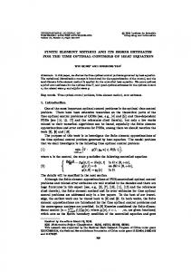
one-level procedure provided by the above mentioned package. All calculations have been carried out on a SGI O2 computer with a MIPS R5000 processor. Figure 1 displays the decadic logarithm of Ks both in two and three dimensions. These values start near −2 (in the blue colored regions) and go up to 2 (in the red part). The reduced saturation in the two-dimensional case is shown in the images on the left in the figures 2 - 4. There the pictures have been rotated clockwise with 90◦ , so the wetting front moves from left to right. Red colored regions are fully saturated, while in the blue ones water is present only at the residual saturation. As expected due to the degenerate character of the problem, the sharp fronts are separating the two regions. The results are in good agreement with those reported in [27] and [26]. The images on the right in the figures 2 - 4 present the results obtained in the three dimensional case. First the absolute permeability is displayed. For the clarity of the image, low permeable zones are set completely transparent, while above a certain value of the permeability the medium reflects the rendering ray. The evolution of the threedimensional wetting front is shown in the last three figures. Again, saturation close to 0 or 1 is set to transparency, so the images display only the wetting front. As in the two-dimensional case, the low to high saturation are transformed in the visualized into blue to red colors. A movie regarding this simulation can be downloaded from http://www.scs.ubbcluj.ro/˜ispop/

Figure 1. Decadic logarithm of Ks , 2 (left) and 3 (right) dimensions.

Error estimates for a time discretization method for the Richards’ equation

15

Figure 2. Reduced saturation, 20, respectively 10 time steps.

Figure 3. Reduced saturation, 20, respectively 10 time steps. Acknowledgements. The author expresses his thanks to Prof. W. J¨ager for suggesting to consider this kind of problems, and to Prof. J. Kaˇcur, Dr. N. Neuß and Dr. C. Wagner for useful discussions. The visualization program for the three dimensional results has been realized by Mr. C. Dˆart¸u. This work was partially supported by the Deutsche Forschungsgemeinschaft, through SFB 359 (sub-project D1) at the Interdisciplinary Center for Scientific Computing (IWR) of the University of Heidelberg, and by the Netherlands Organization for Scientific Research (NWO), through the project 809.62.010 of the Earth and Life Sciences (ALW) research council.

16

I. S. Pop

Figure 4. Reduced saturation, 1000, respectively 30 time steps. References [1] H. W. Alt & S. Luckhaus, Quasilinear elliptic-parabolic differential equations, Math. Z., 183(1983), 311 - 341. [2] R. G. Baca, J. N. Chung & D. J. Mulla, Mixed transform finite element method for solving the nonlinear equation for flow in variably saturated porous media, Int. J. Numer. Meth. Fluids, 24(1997), 441 - 455. [3] P. Bastian, K. Birken, K. Johannsen, S. Lang, N. Neuss, H. Rentz-Reichert & C. Wieners, UG - A flexible software toolbox for solving partial differential equations, Computing and Visualization in Science, 1(1997), 27 - 40. [4] J. Bear & Y. Bachmat, Introduction to Modelling of Transport Phenomena in Porous Media, Kluwer Academic, Dordrecht, 1991. [5] L. Berganaschi & M. Putti, Mixed finite elements and Newton-type linearizations for the solution of Richards’ equation, Int. J. Numer. Meth. Engineering, 45(1999), 1025 - 1046. [6] M. A. Celia, E. T. Bouloutas & R. L. Zarba, A general mass-conservative numerical solution for the unsaturated flow equation, Water Resour. Res., 26(1990), 1483 - 1496. [7] C. J. van Duijn & L. A. Peletier, Nonstationary filtration in partially saturated porous media, Arch Rat. Mech. Anal., 78(1982), 173 - 198. [8] C. M. Elliott, Error analysis of the enthalpy method for the Stefan problem, IMA J. Numer. Anal., 7(1987), 61 - 71. [9] R. Eymard, M. Gutnic & D. Hillhorst, The finite volume method for Richards equation, Comput. Geosci., 3(1999), 259 - 294. [10] M. Th. van Genuchten, A closed-form equation for predicting the hydraulic conductivity of unsaturated soils, Soil Sci. Soc. Am. J., 44(1980), 892 - 898. [11] B. H. Gilding, Qualitative mathematical analysis of the Richards equation, Transport in Porous Media, 5(1991), 651 - 666. [12] W. Hackbusch, On first and second order box schemes, Computing, 41(1989), 277 - 296. [13] J. Hulshof & N. Wolanski, Monotone flows in N-dimensional partially saturated porous media: Lipschitz continuity of the interface, Arch. Rat. Mech. Anal., 102(1988), 287 - 305. [14] W. J¨ager & J. Kaˇcur, Solution of doubly nonlinear and degenerate parabolic problems by relaxation schemes, M2 AN (Math. Model. Numer. Anal.), 29(1995), 605 - 627.

Error estimates for a time discretization method for the Richards’ equation

17

[15] J. Kaˇcur, Solution to Strongly Nonlinear Parabolic Problems by a Linear Approximation Scheme, IMA J. Numer. Anal., 19(1999), 119 - 145. [16] D. Kavetski, P. Binning & S. W. Sloan, Adaptive time stepping and error control in a mass conservative numerical solution of the mixed form of Richards equation, Adv. Water Res. 24(2001), 595 605. [17] C. T. Kelley, C. T. Miller & M. D. Tocci, Termination of Newton/chord iterations and the method of lines, SIAM J. Sci. Comput., 19(1998), 280 - 290. [18] E. Magenes, R. H. Nochetto & C. Verdi, Energy error estimates for a linear scheme to approximate nonlinear parabolic problems, M2 AN (Math. Model. Numer. Anal.), 21(1987), 655 - 678. [19] Y. Mualem, A new model for predicting the hydraulic conductivity of unsaturated porous media, Water Resour. Res., 12(1976), 513 - 522. [20] R. H. Nochetto & C. Verdi, Approximation of degenerate parabolic problems using numerical integration, SIAM J. Numer. Anal., 25(1988), 784 - 814. [21] F. Otto, L1 -contraction and uniqueness for quasilinear elliptic-parabolic equations, J. Differ. Equations, 131(1996), 20 - 38. [22] I. S. Pop, Regularization methods in the numerical analysis of some degenerate parabolic equations, Preprint 98-43 (SFB 359) (1998), IWR, University of Heidelberg. [23] I. S. Pop & W. A. Yong, A numerical approach to porous medium equation, submitted. [24] M. J. L. Robin, A. L. Gutjahr, E. A. Sudicky & J. L. Wilson, Cross-corelated random field generation with the direct Fourier transform method, Water Resour. Res., 29(1993), 2385 - 2397. [25] M. Slodicka, Some finite element schemes arising in modeling of flow through porous media, Habil. Th., University of Augsburg, Germany, 1999. [26] C. Wagner, Numerical methods for diffusion-reaction-transport processes in unsaturated porous media, Computing and Visualisation in Science, 1(1998), 97 - 105. [27] C. Wagner, G. Wittum, R. Fritsche & H. P. Haar, Diffusions-Reaktionsprobleme in unges¨attigten por¨osen Medien, in ”Mathematik-Schl¨ usseltechnologie f¨ ur die Zukunft”, K. H. Hoffmann, W. J¨ager, T. Lohmann & H. Schunck (eds.), Springer Verlag, Berlin, 1997. [28] G. A. Williams & C. T. Miller, An evaluation of temporally adaptive transformation approaches for solving Richards’ equation, Adv. Water Res. 22(1999), 831 - 840. [29] C. S. Woodward & C. N. Dawson, Analysis of expanded mixed finite element methods for a nonlinear parabolic equation modeling flow into variably saturated porous media, SIAM J. Numer. Anal., 37(2000), 701 - 724. [30] E. Zeidler, Applied Functional Analysis, Vols. I, II, Applied Mathematical Sciences 108, 109, Springer Verlag, New York, 1995.