error estimates for the finite element approximation of a ... - TU Berlin

ERROR ESTIMATES FOR THE FINITE ELEMENT APPROXIMATION OF A SEMILINEAR ELLIPTIC CONTROL PROBLEM WITH STATE CONSTRAINTS AND FINITE DIMENSIONAL CONTROL SPACE P. MERINO‡

† ¨ F. TROLTZSCH

B. VEXLER∗

Abstract. The finite element approximation of optimal control problems for semilinear elliptic partial differential equation is considered, where the control belongs to a finite-dimensional set and state constraints are given in finitely many points of the domain. Under the standard linear independency condition on the active gradients and a strong second-order sufficient optimality condition, optimal error estimates are derived for locally optimal controls.

1. Introduction In this paper, we derive error estimates for a finite element based approximation of a semilinear elliptic optimal control problem with control out of a finite-dimensional set and constraints on the state which are required only in finitely many points of the spatial domain. This type of problems is interesting for several reasons. Finite-dimensional controls appear in many real applications of optimal control theory, because it is rather difficult to practically implement control functions that can vary arbitrarily in space. We refer also to [10], where examples of problems with practical importance are mentioned. If pointwise state constraints are given with finite-dimensional control space, then they are often active in finitely many points only. Therefore, finitely many point constraints turn out to be interesting for numerical computations, if the location of active points has been detected. Our problem is equivalent to a nonlinear programming problem in a finite-dimensional space. Therefore, the existence of optimal controls, first-or second-order optimality conditions are more or less standard results since they follow from classical results of mathematical programming after transforming the control problem into a finite-dimensional one. We refer to [10], where optimality conditions for semilinear control problems with finite-dimensional control space are discussed with pointwise state constraints given in the whole spatial domain. The question of error estimates, however, is still interesting. Numerical computations indicate that the numerical approximation of the optimal controls and states is of the order h2 , where h > 0 is the mesh size of the finite element scheme. We can show that the order of the error is equal to h2 | log h|, which corresponds to the error estimate for the finite-element approximation of the state in L∞ -norm. This is quite clear intuitively, since the control space is finite-dimensional and the state constraints are posed pointwise 1

2

P. MERINO‡

† ¨ F. TROLTZSCH

B. VEXLER∗

in a finite number of points. Then, no interpolation error of the optimal control occurs that in the case of control functions limits the order of convergence to h for a cellwise constant approximation of the control variable, see, e.g., [3], and to h3/2 for a piecewise linear approximation, see, e.g., [30] and [13]. For pointwise state constraints in the whole domain, we know only a few results. In Casas [7], the convergence of finite element approximations to optimal control problems for semilinear elliptic equations with finitely many state constraints is proven for piecewise constant approximations of the control function. This result was extended by Casas and Mateos [8] to boundary control problems. Error estimates were derived by Deckelnick and Hinze [11] and Meyer [23], who consider linear-quadratic problems with pointwise state constraints and obtain the order h1−ε for domains of the dimension d = 2 and h1/2−ε for d = 3 under the assumption that the control function is not discretized. Recently, Deckelnick and Hinze [12] estimated the error by h| log h| for d = 2 and h1/2 for d = 3 with piecewise constant approximation of the control. Extending L∞ -error estimates from [27] for linear elliptic equations to the semilinear case, we show that the order is precisely h2 | log h|. At first glance, this is surprising since the Lagrange multipliers associated with the (finitely many) pointwise state constraints are regular Borel measures, which appear in the adjoint equation of the control system. It is the finite-dimensional nature of our problem that explains the high order of the error. This problem of error estimates leads to investigating a perturbed nonlinear programming problem, where the perturbation parameter is the mesh size h – seemingly a standard problem of perturbation analysis. However, we were not able to find approximation results in the literature, which can be applied directly to our problem. In view of this, we include a section on a perturbation result for perturbed nonlinear programming problems, where we also comment on related papers. The paper is organized as follows: In Section 2 we define the optimal control problem (OCP ), introduce the notation and state the assumptions. In Section 3, the finite element discretization is introduced and error estimates for the partial differential equations are derived. Moreover, this section is devoted to estimating the error for the solutions of the optimal control problem. Numerical examples are presented in Section 4, and Section 5 contains the error analysis for perturbed nonlinear programming problems. 2. Optimal control problem and optimality conditions 2.1. Definition of the problem and main assumptions. We consider the following optimal control problem:  Z   min J(yu , u) = L(x, yu (x), u) dx    Ω  u∈Uad subject to (OCP)     gi (yu (xi )) = 0, for all i = 1, . . . , k,   gi (yu (xi )) ≤ 0, for all i = k + 1, . . . , `,

ERROR ESTIMATES: CONTROL WITH FINITE-DIMENSIONAL CONTROL SPACE

3

where yu is the solution to the state equation A y(x) + d(x, y(x), u) = 0 in Ω y(x) = 0 on Γ

(2.1)

and Uad is the set of box constraints defined by Uad = {u ∈ Rm : ua ≤ u ≤ ub } with given vectors ua ≤ ub of Rm . We assume l ≥ 1 and set k = 0, if only inequality constraints are given and k = l, if only equality constraints are given. The set Ω is a convex bounded open set in R2 with boundary Γ. For simplicity, we assume that Γ is polygonal. The extension of some of our results to curved boundaries is possible along the lines of Arada et al. [3]. Moreover, functions L, d : Ω × Rm+1 → R, and gi : R 7→ R of class C 2 are given together with points xi ∈ Ω, i = 1 . . . `. Notice that these points are not located at the boundary of Ω. The operator A is a symmetric uniformly elliptic differential operator of the form Ay(x) = −

n X

∂j (aij (x)∂i y(x))

i,j=1

with coefficients aij ∈ C 1+α (Ω), 0 < α < 1. The control u ∈ Rm is allowed to occur nonlinearly in the state equation, since the controls are vectors. For control functions, the proof of existence would be a delicate issue. Notation: If not stated otherwise, we consider our vectors as column vectors. By | · |, the Euclidean norm of vectors in spaces Rn is denoted, while k · k stands for the norm of matrices (defined by the Euclidean norm of the vector of all entries). The open ball around u in Rm with radius ρ is denoted by B(u, ρ). If f : Rn → R is a twice differentiable function, then f 0 is its derivative and ∇f is the associated gradient, i.e. the representation of f 0 by a column vector. Moreover, f 00 (z) denotes the Hessian matrix of f at the vector z. We denote by c a generic constant, while C is a constant appearing in all estimates of our theorems; it is the maximum of all associated constants. Main assumptions: (A.1) (Carath`eodory type assumptions) For each fixed x ∈ Ω, the functions L = L(x, y, u) and d = d(x, y, u) are of class C 2 with respect to (y, u). For all fixed (y, u) or fixed y, respectively, they are H¨older continuous with respect to the variable x ∈ Ω. (A.2) (Monotonicity) For all x ∈ Ω, all u ∈ Uad and y ∈ R, it holds that ∂d (x, y, u) ≥ 0. ∂y (A.3) (Boundedness and Lipschitz properties) There is a constant C and, for all M > 0,

P. MERINO‡

4

† ¨ F. TROLTZSCH

B. VEXLER∗

a constant cL (M ) > 0 such that the estimates |d(x, 0, 0)| + |d0 (x, 0, 0)| + kd00 (x, 0, 0)k ≤ C kd00 (x, y1 , u1 ) − d00 (x, y2 , u2 )k + kgj00 (y1 ) − gj00 (y2 )k ≤ CL (M )(|y1 − y2 | + |u1 − u2 |) hold for all x ∈ Ω, all ui ∈ Uad and all |yi | ≤ M , i = 1, 2, j = 1, . . . , `. Here, d0 and d00 denote the derivative and the Hessian matrix of d(x, y, u) with respect to (y, u), respectively. The function L is assumed to satisfy (A.3) accordingly. Lemma 1. Under the assumptions (A.1) - (A.3), to each u ∈ Uad there exists a unique ¯ There is a constant C such that kyu kL∞ (Ω) ≤ C is satisfied solution yu ∈ H01 (Ω) ∩ C(Ω). for all u ∈ Uad . If Ω is convex or of class C 2 , then yu belongs to H 2 (Ω). The first part of this result and the uniform boundedness are standard, we refer to Casas [6]. The H 2 -regularity follows from results by Grisvard [17] on linear equations after taking the nonlinear terms with d(·, yu , u) ∈ L∞ (Ω) to the right-hand side of the equation. The state y that is associated to the control u by the PDE in (OCP), is denoted by ¯ i.e. yu = S(u); S is our yu . We denote the mapping u 7→ yu by S : Rm → H01 (Ω) ∩ C(Ω), control-to-state mapping. Lemma 2. Under the assumptions (A.1) - (A.3), the control-to-state mapping S : Rm → ¯ is twice continuously Fr´echet-differentiable. For arbitrary elements u and v H01 (Ω) ∩ C(Ω) m of R , the function zv (u) := S 0 (u)v is given by zv (u) = z, where z is the unique solution to the problem  ∂d ∂d  Az + (x, yu , u) z = − (x, yu , u) v in Ω (2.2) ∂y ∂u  z =0 on Γ, and the inequality kzv (u)kH 1 (Ω) + kzv (u)kC(Ω) (2.3) ¯ ≤ C |v| is satisfied with some constant C that is independent of u ∈ Uad . The function zv1 v2 (u) := S 00 (u)[v1 , v2 ] is obtained by zv1 v2 = z, where z is the unique solution of  ∂d  Az + (x, yu , u) z = −(yv0 1 , v1> ) d00 (x, yu , u) (yv0 2 , v2> )> in Ω (2.4) ∂y  z =0 on Γ with yv0 1 = S 0 (u)(v1 ) and yv0 2 = S 0 (u)(v2 ). For later use of the theory of nonlinear optimization in finite-dimensional spaces, we convert problem (OCP) into a finite-dimensional nonlinear programming problem. We introduce the reduced objective function f : Rm 7→ R of class C 2,1 by f (u) = J(yu , u) = J(S(u), u).

ERROR ESTIMATES: CONTROL WITH FINITE-DIMENSIONAL CONTROL SPACE

5

By our assumptions, in particular the Lipschitz properties of the second derivatives of the given nonlinear functions and the boundedness of Uad , it follows that S 00 is Lipschitz on Uad , i.e. there exists a constant C > 0 such that m kS 00 (u1 )[v1 , v2 ]−S 00 (u2 )[v1 , v2 ]kH01 (Ω)∩C(Ω) ¯ ≤ C|u1 −u2 | |v1 ||v2 | ∀ui ∈ Uad , vi ∈ R . (2.5)

Moreover, we define the restriction function G by G(u) = [g1 (yu (x1 )), . . . , g` (yu (x` ))]> .

(2.6)

An equivalent formulation is G(u) = [g1 (δ1 S(u)), . . . , g` (δ` S(u))]> ,

(2.7)

where δi denotes the Dirac measure concentrated at the point xi , i = 1, . . . , `. It shows that Dirac measures will naturally appear in the adjoint equation associated with (OCP). By these definitions, (OCP) becomes equivalent to the finite-dimensional nonlinear programming problem (NP),  min f (u)     G (u) = 0, i = 1, . . . k, i (N P )  Gi (u) ≤ 0, i = k + 1, . . . `,    u ∈ Uad . Remark 1. This problem admits at least one optimal solution u¯, if its admissible set is non-empty. This follows immediately by the Weierstraß theorem, since f and G are continuous and Uad is compact. Therefore, by its equivalence to (NP), also (OCP) is solvable in this case. 3. The discretized optimal control problem 3.1. Finite element scheme and discretized optimal control problem. To discretize the optimal control problem, we introduce a finite element approximation of the state equation (2.1). We consider a family of meshes {Th }h>0 consisting of triangles T ∈ Th such that ¯ ∪T ∈T T = Ω. h

Notice that Ω was supposed to be polygonal for simplicity. For each triangle T ∈ Th , we introduce the diameter ρ(T ) of T , and the diameter σ(T ) of the largest circle contained in T . The mesh size h is defined by h = maxT ∈Th ρ(T ). We impose the following regularity assumption on the grid: (A.4)

There exist two positive constants ρ and σ such that ρ(T ) ≤ σ and σ(T )

are fulfilled for all h > 0.

h ≤ ρ, ρ(T )

∀T ∈ Th ,

† ¨ F. TROLTZSCH

P. MERINO‡

6

B. VEXLER∗

Associated with the given triangulation Th , we introduce the set of piecewise linear and continuous functions ¯ : yh | ∈ P1 (T ) ∀T ∈ Th , yh = 0 on Γ}, Yh = {yh ∈ C(Ω) T where P1 (T ) denotes the set of affine real-valued functions defined on T . For convenience, we introduce the bilinear form a(y, η) =

Z X n

aij (x)∂xi y ∂xj η dx.

Ω i,j=1

The discrete state yh is defined as the (unique) element of Yh that satisfies the following finite element scheme associated with (2.1): Z a(yh , ηh ) + d(x, yh , u) ηh dx = 0 ∀ ηh ∈ Yh . (3.1) Ω

The following existence and approximation result was proven in [9] for distributed control functions in Lipschitz domains. It is obvious that it remains valid without changes for our case with control vectors. It shows that the discretized equation is well posed. Theorem 1. Let the assumptions (A.1)–(A.3) and (A.4) be satisfied. Then, for all u ∈ Uad , the equation (3.1) has a unique solution yh,u ∈ Yh . There exists a constant C independent of h and u ∈ Uad such that, with n = dim Ω, kyu − yh,u kL2 (Ω) ≤ C h2 kyu kH 2 (Ω) kyu − yh,u kL∞ (Ω) ≤ C h2−n/2 kyu kH 2 (Ω) .

(3.2) (3.3)

To indicate the correspondence of yh to u, we will denote this solution also by yh,u . The mapping u 7→ yh,u is denoted by Sh . We will improve estimate (3.3) in an interior subdomain Ω0 containing the points xi , where the state constraints are required. We approximate (OCP) by substituting the discretized equation (3.1) for the state equation. We study the following (discretized) finite-dimensional control problem Z   min J(yh,u , u) = L(x, yh,u (x), u) dx    u∈Uad Ω (3.4) (OCPh )  gi (yh,u (xi )) = 0 for all i = 1, . . . , k,    gi (yh,u (xi )) ≤ 0 for all i = k + 1, . . . , `. Let us define fh (u) = J(yh,u , u),

Gh (u) = [g1 (yh,u (x1 )), . . . , g` (yh,u (x` ))]> .

ERROR ESTIMATES: CONTROL WITH FINITE-DIMENSIONAL CONTROL SPACE

7

By these terms, we transform the problem (3.4) to the finite-dimensional nonlinear programming problem  min fh (u)     G (u) = 0, i = 1, . . . k, h,i (N Ph ) (3.5)  Gh,i (u) ≤ 0, i = k + 1, . . . `,    u ∈ Uad . ¯ 0 ⊂ Ω be a subdomain of Ω that 3.2. Improved L∞ -error estimate. Let Ω0 with Ω contains all given points xi , i = 1, . . . , `. The main goal of this subsection is to estimate the L∞ -norm of the difference yu − yh,u in Ω0 . We rely on an associated estimate for linear equations from [27] and on Theorem 1 by Casas and Mateos [9]. An estimate of the order h2 | log(h)| was derived in [27] for compact subdomains of polygonal domains. We also mention the related papers [26] and [15], where the error estimate h2 | log(h)| was shown for domains with sufficiently smooth boundary. Another technique for proving local error estimates with respect to the L∞ -norm is presented in [31, 32]. Here, we extend the result of [27] to the semilinear case. ¯ 0 ⊂ Ω1 and Ω ¯ 1 ⊂ Ω. First, we show that the state yu belongs to W 2,∞ (Ω1 ), where Ω Lemma 3. Under the assumptions (A.1)-(A.3), the state yu belongs to W 2,∞ (Ω1 ) for all u ∈ Uad . Proof. We already know that yu is bounded and measurable, hence the same is true for d(·, yu , u). Writing the state equation in the form Ayu = −d(·, yu , u), we see that yu solves a linear elliptic equation with right-hand side in L2 (Ω). Since Ω is convex and bounded, yu ∈ H 2 (Ω) follows from Grisvard [17], hence yu is H¨older continuous, because Ω is two¯ dimensional. The smoothness and Lipschitz assumptions on d ensure d(·, yu , u) ∈ C 0,κ (Ω). with some κ ∈ (0, 1). Therefore, yu solves a linear elliptic boundary value problem Ayu = f,

yγ = 0

with H¨older continuous right-hand side f and continuous boundary data. As a convex bounded domain, Ω satisfies the exterior sphere condition. In view of this, we can apply Theorem 6.13 by Gilbarg and Trudinger [16] and obtain yu ∈ C 2,α (Ω) with some α ∈ (0, 1). ¯ 1 ), hence the statement of the Lemma is true.  This implies in particular yu ∈ C 2,α (Ω Now we are going to derive a uniform error estimate of the order h2 | log h| in Ω0 . The following estimate is known, e.g., from [27], for the linear case, cf. also [31, 32]: kyh,u − yu kC(Ω0 ) ≤ C h2 | log h| (kyu kW 2,∞ (Ω1 ) + kyu kH 2 (Ω) ),

(3.6)

¯ 0 ⊂ Ω1 and Ω ¯ 1 ⊂ Ω. We shall extend this estimate to the semilinear equation (2.1). where Ω To establish our error estimate, we rely on the following stability result for linear elliptic equations from [27]:

P. MERINO‡

8

† ¨ F. TROLTZSCH

B. VEXLER∗

¯ 0 ⊂ Ω1 and Ω ¯ 1 ⊂ Ω and assume that Theorem 2. Let Ω1 be a subdomain of Ω with Ω ¯ are given. If zh ∈ Yh is the solution of B ∈ (W 1,∞ (Ω))2×2 and ψ ∈ H01 (Ω) ∩ C(Ω) a(zh , ηh ) = (B∇ψ, ∇ηh ) ∀ηh ∈ Yh , then there holds
kzh kL∞ (Ω0 ) ≤ c kBkW 1,∞ (Ω) | log(h)|kψkL∞ (Ω1 ) + kψkL2 (Ω) + h kψkH 1 (Ω) . Our main error estimate for the state equation is expressed by the following result: Theorem 3. Let Ω0 and Ω1 be defined as in Theorem 2. Then there exists a constant C > 0, independent of h and u ∈ Uad such that it holds
kyu − yh,u kL∞ (Ω0 ) ≤ C h2 | log h| kyu kW 2,∞ (Ω1 ) + h2 kyu kH 2 (Ω) . Proof. In the proof, we keep the control u in (2.1) fixed. In view of this, we denote yu by y and yh,u by yh to simplify the notation. (i) The state yu is bounded, hence the L∞ -estimate (3.3) implies uniform boundedness of yh , independently of h. Therefore, we get from the Lipschitz continuity of d with respect to y and from the estimate (3.2) kd(·, y, u) − d(·, yh , u)kL2 (Ω) ≤ c ky − yh kL2 (Ω) ≤ c h2 kykH 2 (Ω) .

(3.7)

We consider an intermediate solution y˜h ∈ Yh determined by a(˜ yh , ηh ) = −(d(·, y, u), ηh ) ∀ηh ∈ Yh , where (· , ·) denotes the inner product of L2 (Ω). It is clear that y satisfies the same equation, hence a(˜ yh , ηh ) = a(y, ηh ) ∀ηh ∈ Yh . Inserting the interpolate ih y of y, we obtain a(ih y − y˜h , ηh ) = a(ih y − y, ηh ) ∀ηh ∈ Yh . Now we apply Theorem 2 to ψ = ih y − y and deduce
kih y − y˜h kL∞ (Ω0 ) ≤ c | log h| kih y − ykL∞ (Ω1 ) + kih y − ykL2 (Ω) + hkih y − ykH 1 (Ω) . (3.8) Due to known properties of the interpolation operator, cf. Brenner and Scott [5], we have kih y − ykL2 (Ω) + h kih y − ykH 1 (Ω) ≤ c h2 kykH 2 (Ω) kih y − ykL∞ (Ωi ) + h kih y − ykW 1,∞ (Ωi ) ≤ c h2 kykW 2,∞ (Ωi ) ,

i = 0, 1.

Using these interpolation estimates in (3.8), we arrive at
ky − y˜h kL∞ (Ω0 ) ≤ c h2 | log h| kykW 2,∞ (Ω1 ) + h2 kykH 2 (Ω) .

(3.9)

(ii) It remains to estimate the error vh = y˜h − yh ∈ Yh . Subtracting the equations for y˜h and yh , we find that vh solves a(vh , ηh ) = (d(·, yh , u) − d(·, y, u), ηh ) ∀ηh ∈ Yh . ¯ defined by Now consider the function v ∈ H01 (Ω) ∩ C(Ω) a(v, η) = (d(·, yh , u) − d(·, y, u), η) ∀η ∈ H01 (Ω).

ERROR ESTIMATES: CONTROL WITH FINITE-DIMENSIONAL CONTROL SPACE

9

Obviously, vh is the discrete solution belonging to v. From standard estimates for linear elliptic equations and from inequality (3.7), it follows that kvkL∞ (Ω) + kvkH 1 (Ω) ≤ c kd(·, y, u) − d(·, yh , u)kL2 (Ω) ≤ c h2 kykH 2 (Ω) . Now, we apply Theorem 2 to the linear equation a(vh , ηh ) = a(v, ηh ) ∀ηh ∈ Yh and obtain
kvh kL∞ (Ω0 ) ≤ c | log(h)|kvkL∞ (Ω1 ) + kvkL2 (Ω) + h kvkH 1 (Ω) ≤ c | log(h)| h2 kykH 2 (Ω) . In view of (3.9), the inequality ky − yh kL∞ (Ω0 ) ≤ ky − y˜h kL∞ (Ω0 ) + kvh kL∞ (Ω0 ) yields the statement of the theorem.  3.3. Application to the optimal control problem. Let us first summarize the error estimates of the preceding subsection in the following lemma: Lemma 4. Let yu and yh,u be the solutions of the equations (2.1) and (3.1), respectively. Let zv (u) solve (2.2) and zv,h (u) satisfy the corresponding discretized equation. Then there exists a constant C > 0, independent of h, such that the estimates kyu − yh,u kC(Ω¯ 0 ) ≤ C h2 | log h| 2

kzv (u) − zv,h (u)kC(Ω¯ 0 ) ≤ C h | log h||v|

(3.10) (3.11)

hold for all u ∈ Uad , v ∈ Rm and h > 0. Proof. Lemma 1 and the Lipschitz properties of d ensure the existence of a bound M > 0 with kd(·, yu , u)kL2 (Ω) ≤ M for all u ∈ Uad . In view of this and by Lemma 3, kyu kH 2 (Ω) and kyu kW 2,∞ (Ω1 ) are uniformly bounded for all u ∈ Uad and (3.10) is an immediate conclusion of Theorem3. Estimate (3.11) follows from (3.10) as in [3], Proposition 7.1. Notice that, due to the boundedness of Uad , the functions yu and yh,u belong to a bounded set. This is used for the proof in [3].  Lemma 4 implies an estimate of G − Gh in the C 2 -norm: Lemma 5. Under the assumptions (A.1)–(A.3) and (A.4), there is a constant C > 0 such that |G(u) − Gh (w)| + kG0 (u) − G0h (w)k+ ` X + kG00i (u) − G00h,i (w)k ≤ C(|u − w| + h2 | log h|)

(3.12)

i=1

holds for all u, w in Uad . Proof. Let c denote a generic constant. Taking into account that all gi are of class C 2,1 , hence also the functions Gi , in view of Lemma 4 we have |Gi (u) − Gh,i (w)| = |gi (yu (xi )) − gi (yh,w (xi ))| ≤ c kyu − yh,w kC(Ω¯ 0 ) ≤ c kyu − yw kC(Ω¯ 0 ) + c kyw − yh,w kC(Ω¯ 0 )

10

P. MERINO‡

† ¨ F. TROLTZSCH

≤ c |u − w| + c h2 | log h|

B. VEXLER∗

∀i = 1, . . . , `,

where the last inequality is obtained since the mapping u 7→ yu is Lipschitz. For the derivative G0 , we argue similarly. Let w be an arbitrary unit vector of Rm . Then 0 Gi (u)v − G0h,i (w)v ≤|G0i (u)v − G0i (w)v| + G0i (w)v − G0h,i (w)v ≤|gi0 (yu (xi )) (S 0 (u)v) (xi ) − gi0 (yw (xi )) (S 0 (w)v) (xi )| + |gi0 (yw (xi )) (S 0 (w)v) (xi ) − gi0 (yh,w (xi )) (Sh0 (w)v) (xi )| ≤c kgi0 (yu )zv (u) − gi0 (yw )zv (w)kC(Ω¯ 0 ) + kgi0 (yw )zv (w) − gi0 (yh,w )zh,v (w)kC(Ω¯ 0 ) , where zv (u) and zv (w) are defined as in Theorem 2 and zh,v (w) is the discrete state associated with zv (w). With a constant C we obtain that kyu − yw kC(Ω¯ 0 ) ≤ C |u − w|,

kyw − yh,w kC(Ω¯ 0 ) ≤ C h2 | log h|

kzv (w) − zh,v (w)kC(Ω¯ 0 ) ≤ C h2 | log h| |v| for all u, w ∈ Uad and all v ∈ Rm . The first inequality expresses the Lipschitz continuity of u 7→ yu , while the second and third one follow from Lemma 4. The estimates for G and G0 are deduced now immediately from the estimates above. For G00 , the technique is analogous to the one for G0 , since kzv1 v2 (w) − zh,v1 v2 (w)kC(Ω¯ 0 ) ≤ C h2 | log h| |v1 ||v2 | follows from equation (2.2) that has the same structure as (2.4).  Lemma 6. Under the assumptions of Lemma 5, the estimate |f (u) − fh (u)| + |f 0 (u) − fh0 (u)| + kf 00 (u) − fh00 (u)k ≤ C h2

∀u ∈ Uad

is satisfied with some constant C not depending on h and u. Proof. The function L is Lipschitz on bounded sets and, in view of Lemma 1 and (3.3), kyu kC(Ω) ¯ and kyh,u kC(Ω) ¯ are uniformly bounded for all u ∈ Uad and all h. Therefore, we find Z |fh (u) − f (u)| ≤ |L(x, yh,u , u) − L(x, yu , u)| dx ≤ c kyh,u − yu kL2 (Ω) ≤ Ch2 Ω

by (3.2). Similarly, we can estimate the second part  Z  ∂L ∂L 0 0 (f (u) − fh (u))v = (x, yu , u)zv (u) − (x, yh,u , u)zh,v (u) dx ∂y ∂y Ω  Z  ∂L ∂L + (x, y, u)v − (x, yh,u , u)v dx ∂u ∂u Ω by (3.2) and the associated L2 -version of (3.11), kzv (u) − zv,h (u)kL2 (Ω) ≤ C h2 |v| for all unit vectors v. As in the last proof, the estimation of kf 00 (u) − fh00 (u)k is analogous to that of |f 0 (u) − fh0 (u)|. 

ERROR ESTIMATES: CONTROL WITH FINITE-DIMENSIONAL CONTROL SPACE

11

Let us now state the main result of our paper, an error estimate for optimal controls of the discretized optimal control problem (OCPh ). This estimate follows from our error analysis for nonlinear mathematical programming problems in Section 5 as a corollary of Theorem 8 applied to (NP) and (NPh ). The essential assumptions (LICQ) and (5.24) are formulated later in Section 5, but we found it reasonable to present our main result already here. Theorem 4. Assume that the assumptions (A.1)-(A.4) are fulfilled and let u¯ be a locally optimal control of problem (OCP) satisfying the linear independence condition (LICQ) of Definition 3 along with the strong second-order condition (5.24). Then u¯ is locally unique and there exists a sequence u¯h of locally optimal controls of the corresponding FEM-approximated problem (OCPh ) and a constant C > 0 independent of h such that the estimate |¯ u − u¯h | ≤ C h2 | log h|. (3.13) is satisfied for all sufficiently small h. Proof. The optimal control problems (OCP) and (OCPh ) are equivalent to the nonlinear programming problems (NP) and (NPh ), which are particular cases of the nonlinear programming problems (P) and (Ph ), which will be discussed in Section 5. Due to the previous error estimates, assumption (A.5) is fulfilled with α(h) = h2 | log h|. Therefore, Theorem 8 is applicable to (NP) and (NPh ) and Theorem 4 is a direct conclusion.  Remark 2. The same estimate holds true for the vectors of Lagrange multipliers ν¯ and ν¯h associated with u¯ and u¯h , i.e. |¯ ν − ν¯h | ≤ C h2 | log h|. These multipliers are associated with the state and control constraints, cf. Theorem 8. 4. Numerical Examples In this section we present numerical test examples for which we confirm error estimates of an order close to α(h) = h2 . This does not contradict our theory, since the | log h|-term can hardly be detected numerically. Notice that h2 log h ≤ c h2−ε holds for all ε > 0. In the test runs, regular triangulations of the domain were generated by the Matlab pde-toolbox command initmesh and successively refined using the command refmesh. The discretized nonlinear optimal control problems were solved by an SQP method where the associated nonlinear programming problems were treated on using the OOQP 1 solver. The right-hand side of the state equation was assembled in an exact fashion, i.e. we do not approximate the integral term involving functions ei , i = 1, . . . , 3, because our theory does not include approximation Z errors for integrals. Therefore, the corresponding right-hand side variational terms ei ηk dx, where ηk , k = 1, . . . , nh are the piecewise linear basis Ω 1OOQP:

Object Oriented Software for Quadratic Programming, Mike Gertz, Steve Wright. http://pages.cs.wisc.edu/ swright/ooqp/. OOQP is copyrighted to the University of Chicago.

12

P. MERINO‡

† ¨ F. TROLTZSCH

B. VEXLER∗

functions of Yh , were assembled computing the corresponding primitive over its limits in each triangle. The experimental error of convergence is computed by EOC =

log(|u − uh1 |) − log(|u − uh2 |) , log(h1 ) − log(h2 )

for two consecutive mesh sizes h1 and h2 . Example 1. This is a slight modification of an example in [24], where the optimal state is active in one single point. The semilinear state equation is considered in the open unit disk Ω = B1 (0).  1 1  min3 J(y, u) = ky − yd k2L2 (Ω) + |u − ud |2    u∈R 2 2       subject to (E1) (4.1) P3 3  −∆y(x) + y(x) + y(x) = u Ω i ei (x) in  i=1    y(x) = 0 on Γ,      y(0, 0) ≤ 1, where e1 (x) = 1, e2 (x) = x21 + x22 , the optimal functions

e3 (x) = (1 − x21 − x22 )3 . In this case, we construct

y¯ = 1 − (x21 + x22 )

and

u¯ = [5, −1, 1]> .

The active set consists of one single point x = (0, 0). The Lagrange multiplier µ = δ0 satisfies the complementarity condition, where δ0 is the Dirac measure concentrated at the 1 origin. If we define ϕ¯ = − log |x|, then we have that 2π
1 −∆ϕ¯ + ϕ¯ + 3¯ y 2 ϕ¯ = δ0 − log |x| 1 + 3(1 − |x|2 )2 , 2π and it is easy to confirm that the right-hand side of this identity is equal to y¯ − yd + µ ¯, if we set
1 yd = 1 − |x|2 + log |x| 1 + 3(1 − |x|2 )2 . 2π The gradient equation for u¯ is satisfied, if we define 1 1 25 > ud = [5, −1, 1]> + [ , , ] . 4 16 192 The numerically computed optimal state and the desired state are shown in Figure 1. Notice that the state is active in the point (0, 0). In Figure 2, the computed Lagrange multiplier and the computed adjoint state are presented. The multiplier has a peak shape concentrated at (0, 0). This reflects the approximation of the Dirac measure δ0 , which is the exact Lagrange multiplier.

ERROR ESTIMATES: CONTROL WITH FINITE-DIMENSIONAL CONTROL SPACE

13

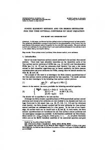
Figure 1. Example 1; − log(h) versus − log(|¯ u − u¯h |) (solid line) compared with −2 log(h) (dashed line) h 0.08192427 0.05016470 0.02508235 0.01263883 0.00633700 0.00317013

|¯ u − u¯h | 0.96438176 0.19273740 0.05252443 0.01450992 0.00405185 0.00119422

EOC 3.28 1.88 1.86 1.85 1.76

Figure 2. Example 1; Numerically computed optimal state y¯h and shift yd for h ≈ 0.0006 Example 2. Here, the state equation contains a the nonlinearity of the type y 2 . Since y 2 is not monotone, it is replaced by the monotone function y |y| for formal reasons. In the numerical computations, this does not matter, because the states turned out to be non-negative. We require that the optimal state y¯ is active at five given points inside the

P. MERINO‡

14

† ¨ F. TROLTZSCH

B. VEXLER∗

Figure 3. Example 1; Numerically computed Lagrange multiplier µ ¯h and adjoint state ϕ¯h for h ≈ 0.0006 domain Ω = (−1, 1) × (−1, 1). The problem reads  1 1   min5 J(y, u) = ky − yd k2L2 (Ω) + |u − ud |2   u∈R 2 2      subject to       −∆y(x) + y(x)(15 + |y(x)|) = P5 u e (x) in Ω i=1 i i (E2) (4.2) y(x) = 0 on Γ,        y(xi ) 6 8/27, i = 1, . . . , 4, and y(x5 ) > 0,      with    x1 = ( √13 , √13 ), x2 = (− √13 , √13 ), x3 = ( √13 , − √13 ), x4 = (− √13 , − √13 ), x5 = (0, 0), and e1 (x) = 12x21 x22 − 2(x41 + x42 ), e2 (x) = x21 + x22 , e3 (x) = 1, e4 (x) = (x21 − 1)(x22 − 1)(x21 + x22 ), e5 (x) = (x21 − 1)2 (x22 − 1)2 (x21 + x22 )2 . We define y¯ = (x21 − 1)(x22 − 1)(x21 + x22 ),

u¯ = [−2, 16, −4, 15, 1]>

so that y¯ is the state associated with u¯. Moreover, we set yd := y¯, ud := u¯ so that y¯ and u¯ are the optimal state and the optimal control, respectively. Obviously, the associated adjoint state is ϕ¯ = 0. Consider the set   1 1 1 1 1 1 1 1 ( √ , √ ), (− √ , √ ), ( √ , − √ ), (− √ , − √ ), (0, 0) , 3 3 3 3 3 3 3 3 8 where the function y¯ attains its maximal value 27 in the first four points, while y¯ reaches its minimum value 0 at the point (0, 0). In view of this choice, y¯ is active at the five points,

ERROR ESTIMATES: CONTROL WITH FINITE-DIMENSIONAL CONTROL SPACE

15

if the state constraints are chosen as above. Therefore, y¯ and u¯ are also the solution for the state-constrained problem. The gradient equation of the optimality system is Z u¯ − ud +

>

Z ϕe ¯ 1 dx, . . . ,

Ω

ϕe ¯ 5 dx

= 0.

(4.3)

Ω

In the computations, we chose an initial mesh that contains the five points where the state is active. Then all refined meshes automatically contain these 5 points. The computed rates for the error are listed in the following table.

Figure 4. Example 2; − log(h) versus − log(|¯ u − u¯h |) (solid line) compared with −2 log(h) (dashed line) h 0.057005028172390 0.028502514086195 0.014251257043098 0.007125628521549 0.003562814260775

|¯ u − u¯h | 0.880415806738625 0.251486866293358 0.063324994190674 0.015606473275112 0.003822447895272

EOC 1.81 1.99 2.02 2.03

Figure 5 shows the numerically computed optimal state, and the Lagrange multiplier is represented in Figure 6. It exhibits peaks in the points where the state is active, this is what we expected from the right-hand side in the adjoint equation (5.5) where Dirac measures are concentrated at the active points. 5. Error estimates for a perturbed nonlinear programming problem 5.1. The programming problem and its perturbation. In the preceding section, we have transformed our elliptic optimal control problem into the nonlinear programming problem (NP). Associated with (NP), a discretized control problem was constructed that is equivalent to the programming problem (NPh ). We are interested in estimating the difference between local solutions of (NP) and associated solutions of (NPh ).

16

P. MERINO‡

† ¨ F. TROLTZSCH

B. VEXLER∗

Figure 5. Example 2; Numerically computed optimal state, and adjoint state at h ≈ 0.005

Figure 6. Example 2; Numerically computed Lagrange multipliers at h ≈ 0.005 This question leads to the sensitivity analysis of nonlinear programming problems with respect to perturbations. Although this issue was the subject of various papers, in most of the references we found, the dependence of the given functions with respect to h is assumed to be Lipschitz or even smoother, because Lipschitz stability or differentiability of the solutions with respect to h was the main interest. In our case, h is a mesh parameter, and the geometry of the grid depends on the distance and on the number of mesh points. The only property we have at our disposal is the continuity of the data at h = 0 with some associated rate. Results contained in

ERROR ESTIMATES: CONTROL WITH FINITE-DIMENSIONAL CONTROL SPACE

17

Bonnans and Shapiro [4], Klatte und Kummer [19], Malanowski [21] or in many of the references cited therein, cannot be directly used, although their techniques need only a slight modification to be applied to our setting. Similarly, the results presented in Alt [2], Klatte [18] or Malanowski et al. [22], would need some adaptation and the verification of the assumptions stated therein. These papers only assume a rate of continuity w.r. to h at h = 0. Therefore, although our arguments are close to the ones of [2], [18] or [22], we decided to work out the error analysis in a fairly selfcontained way for the convenience of the reader. We underline that our perturbation analysis is inspired by the cited references and is based on standard conclusions. In particular, we were partially guided by the work [2]. The error analysis is discussed under assumptions, which are satisfied by our problems (NP) and (NPh ) related to (OCP) and (OCPh ). We discuss the following standard class of nonlinear programming problems that is not necessarily related to (OCP) or (OCPh ), although we use the same notation. We consider  min f (u)     G (u) = 0, i = 1, . . . k, i (P )  Gi (u) ≤ 0, i = k + 1, . . . `,    u ∈ Uad and its perturbed version

(Ph )

 min fh (u)     G (u) = 0, h,i  G h,i (u) ≤ 0,    u ∈ Uad ,

i = 1, . . . k, i = k + 1, . . . `,

where Uad ∈ Rm is the convex and bounded box-shaped set introduced in Section 1, and f, fh , Gi , Gh,i : Rm → R, i = 1, . . . , `, h > 0 are functions of C 2,1 (Uad ). We assume that the following approximation assumption is satisfied: (A.5) There exist a constant C > 0 and a function α : R+ → R+ with α(h) → 0 as h → 0 such that ` P |f (u) − fh (w)| + |f 0 (u) − fh0 (w)| + kf 00 (u) − fh00 (w)k + (|Gi (u) − Gh,i (w)|+ i=1
+|G0i (u) − G0h,i (w)| + kG00i (u) − G00h,i (w)k ≤ C (|u − w| + α(h))

holds for all h > 0 and all u, w ∈ Uad . Notice that (A.5) is satisfied for the problems (NP) and (NPh ) by α(h) = h2 | log h|. To cover the given equality and inequality constraints in a unified way, we introduce the cone K of ”nonnegative” vectors by K = {z ∈ R` : zi = 0, i = 1, . . . k, zi ≥ 0, i = k + 1, . . . , `}.

18

P. MERINO‡

† ¨ F. TROLTZSCH

B. VEXLER∗

Then the constraints Gi (u) = 0, i = 1, . . . k, Gi (u) ≤ 0, i = k + 1, . . . , `, can be expressed by G(u) ≤K 0, where z ≤K 0 ⇔ −z ∈ K. Moreover, we introduce G(u) = [G1 (u), . . . G` (u)]> and define Gh analogously. By these definitions, (P) and (Ph ) can be written as   min f (u) min fh (u) (P ) and (Ph ) G(u) ≤K 0, u ∈ Uad Gh (u) ≤K 0, u ∈ Uad . 5.2. First- and second-order optimality conditions. 5.2.1. First-order necessary conditions. Let us assume once and for all that u¯ is a locally optimal solution to (P). According to Robinson [28], we require the following regularity condition at u¯: 0 ∈ int {G(¯ u) + G0 (¯ u)(Uad − u¯) + K}, (5.1) 0 where the set in braces is defined as ∪{G(¯ u) + G (¯ u)(u − u¯) + k | u ∈ Uad , k ∈ K}. A vector u¯ that satisfies all constraints of (P) and the condition (5.1) is said to be regular. Definition 1. The Lagrange function L : Rm × R` → R associated with (P ) is defined by L(u, µ) = f (u) +

` X

µi Gi (u).

(5.2)

i=1

The well known first-order conditions for (P) are stated in the following theorem. Theorem 5. Suppose that u¯ is locally optimal for (P ) and regular. Then there exists a vector µ ¯ ∈ R` with µi > 0, i = k + 1, . . . , `, such that the variational inequality ∂L (¯ u, µ ¯)(u − u¯) ≥ 0 ∀u ∈ Uad (5.3) ∂u is satisfied together with the complementary slackness conditions µ ¯i Gi (¯ u) = 0

for

i = k + 1, . . . , `.

(5.4)

These relations express the standard necessary first-order conditions of nonlinear programming. The existence of Lagrange multipliers follows from the Robinson regularity condition (5.1). This condition is equivalent to the well known regularity condition by Kurcyusz and Zowe [34] that is sufficient for the existence of Lagrange multipliers (and optimality conditions in qualified form). Remark 3. In the particular case of (NP) that is related to the optimal control problem (OCP), the necessary conditions (5.3)–(5.4) can be expressed in terms of optimal control: We define an adjoint state ϕ ∈ W01,σ (Ω), 1 ≤ σ < n/(n − 1), as the unique solution of the adjoint equation  ` X  ∂L ∂d  (x, y¯, u¯)ϕ = (x, y¯, u¯) + Aϕ + µ ¯i gi0 (¯ y (xi ))δxi in Ω (5.5) ∂y ∂y i=1   ϕ =0 on Γ.

ERROR ESTIMATES: CONTROL WITH FINITE-DIMENSIONAL CONTROL SPACE

19

Then the variational inequality (5.3) can be written as dT (u − u¯) > 0 ∀u ∈ Uad , where d ∈ Rm is defined by d = (di ) with  Z  ∂L ∂d di := (x, y¯, u¯) − ϕ(x) (x, y¯(x), u¯) dx, ∂ui ∂ui Ω

i = 1, . . . , m.

(5.6)

5.2.2. Second-order sufficient conditions. Let us also briefly recall the known second-order conditions. We assume that u¯ satisfies the first-order necessary optimality conditions (5.3) and (5.4) together with the constraints of (P). To formulate the second-order conditions, we need the critical cone Cu¯ . For this purpose we define the index sets associated with the inequality constraints that are included in G(u) ≤K 0 or are defining Uad : I0 := I+ := I0,a := I+,a := I0,b := I+,b :=

{i ∈ {k + 1, . . . , `} : Gi (¯ u) = 0} {i ∈ {k + 1, . . . , `} : µ ¯i > 0} {i ∈ {1, . . . , k} : u¯i = uai } {i ∈ {1, . . . , k} : di > 0} {i ∈ {1, . . . , k} : u¯i = ubi } {i ∈ {1, . . . , k} : di < 0},

where di := ∇u L(¯ u, µ ¯)i . It is a standard conclusion from the variational inequality (5.3) that u¯i = uai must hold for those i with di > 0 and u¯i = ubi for the i with di < 0. The set I+,a ∪ I+,b is often said to be the set of strongly active control constraints. Definition 2. The critical cone Cu¯ is the set of all vectors u ∈ Rm that satisfy the following relations: u) u = 0 G0i (¯ u) u ≤ 0 G0i (¯ ui = 0 ui > 0 ui ≤ 0

for for for for for

all all all all all

i ∈ {1, . . . , k} ∪ I+ i ∈ I0 \I+ i ∈ I+,a ∪ I+,b i ∈ I0,a \I+,a i ∈ I0,b \I+,b .

y (xi ))z(xi ) for all u) u = gi0 (¯ Remark 4. In the case of problem (NP), it holds that G0i (¯ i = 1, . . . , `, where z solves the linearized equation (2.2) with v = u, so that all derivatives above can be expressed in terms of the partial differential equation. Following the theory of second-order conditions in finite-dimensional spaces, cf. Bonnans and Shapiro [4], Luenberger [20] or Fiacco and McCormick [14], we require the following condition: (A.6) The coercivity property uT L00 (¯ u, µ ¯)u > 0 is fulfilled for all u ∈ Cu¯ \ {0}.

20

P. MERINO‡

† ¨ F. TROLTZSCH

B. VEXLER∗

Here and in the following, L00 (u, µ) denotes the Hessian matrix of L at (u, µ) with respect to u. Theorem 6. Let u¯ satisfy the constraints of (P), the first-order necessary conditions (5.3) – (5.4), and the second-order sufficient condition (A.6). Then there exist real numbers ω > 0 and ε > 0 such that f (u) − f (¯ u) > ω|u − u¯|2

(5.7)

holds for all admissible u with |u − u¯| ≤ ε. This is a standard result of nonlinear programming theory, cf. [14] or [20]. To perform our perturbation analysis, we also need the well known linear independence ˆ condition. We extend the vector G(u) to G(u) ∈ R`+2m by G`+i (u) = ua,i − ui ,

for i = 1, . . . , m

G`+m+i (u) = ui − ub,i ,

for i = 1, . . . , m.

Definition 3. The index set A(¯ u) of active constraints at u¯ is defined by A(¯ u) = {i ∈ {1, . . . , ` + 2m} : Gi (¯ u) = 0} . We say that the linear independence constraint qualification (LICQ) holds at u¯ if the vectors ∇Gi (¯ u) of the set of active gradients {∇Gi (¯ u) | i ∈ A(¯ u)} are linearly independent. Remark 5. For all i > `, the gradients ∇Gi (¯ u) are unit vectors with respect to the standard basis multiplied by 1 or −1. Therefore, it is easy to see that the associated active gradients form a system of linearly independent vectors. In view of this, the condition (LICQ) amounts to the requirement that set of vectors defined by the first ` components of the active gradients ∇G(¯ u)i , i ≤ ` is linearly independent. 5.3. Perturbation analysis. To set up the first order-necessary conditions for (Ph ), we introduce the associated Lagrange function Lh : Rm+` → R by Lh (u, µ) = fh (u) + Gh (u)> µ. Then the first-order conditions can be formulated as follows: If u¯h is locally optimal for (Ph ) and the Robinson regularity condition (5.1) is satisfied at u¯ with Gh (¯ uh ) and G0h (¯ uh ) substituted for G(¯ u) and G0 (¯ u), respectively, then there exists a Lagrange multiplier µ ¯h ∈ R` with µ ¯h,i > 0, i = k + 1, . . . , `, such that ∂Lh (¯ uh , µ ¯h )(u − u¯h ) ≥ 0 ∀u ∈ Uad ∂u

(5.8)

µ ¯h,i Gh,i (¯ u) = 0

(5.9)

and for all i = 1, . . . , `.

Lemma 7. If u¯ satisfies the Robinson regularity condition for (P ), then this condition is also fulfilled for all u with |u − u¯| ≤ ρ and all sufficiently small h > 0, if ρ is taken sufficiently small.

ERROR ESTIMATES: CONTROL WITH FINITE-DIMENSIONAL CONTROL SPACE

21

Proof. Obviously, the Robinson regularity condition holds if and only if a small cuboid with the corners c1 , . . . , cn and the origin in its interior is covered by G(¯ u) + G0 (¯ u)(Uad − u¯) + K. We have ci = G(¯ u) + G0 (¯ u)(ui − u¯) + ki ,

i = 1, . . . , n,

with ui ∈ Uad and ki ∈ K. The cuboid is the convex hull of the corners ci . We consider now the points ch,i = Gh (u) + G0h (u)(ui − u) + ki ,

i = 1, . . . , n. P Let ε > 0 be given. Then for sufficiently small ρ and h, we have ni=1 |ci − ch,i | < ε. If ε is small enough, then the convex hull co {ch,1 , . . . , ch,n } contains the origin in its interior. Therefore, 0 ∈ int co {ch,1 , . . . , ch,n } = Gh (u) + G0h (u)(co {u1 , . . . , un } − u) + co {k1 , . . . , kn } ⊂ Gh (u) + G0h (u)(Uad − u) + K so that the Robinson constraint qualification is satisfied.



In view of this Lemma, to each local solution u¯h of (Ph ) sufficiently close to u¯, there exists a Lagrange multiplier, if h is small enough. However, we have to show the existence of a locally optimal u¯h in a neigborhood of u¯ and we want to get an estimate for the difference. We proceed as follows: In a preparatory step, via p Lemma 7 – Lemma 9, we show the existence of u¯h and the estimate (5.19) of the order α(h). This step is inspired by techniques used in Alt [2] and Allgower et al. [1]. Next, we invoke the stability theory for generalized equations to derive an estimate of the order α(h). First, we approximate admissible vectors for (P) by admissible ones for (Ph ) having a distance bounded by c α(h) and vice versa. Lemma 8. Suppose that u¯ is feasible for (P ) and satisfies the Robinson regularity condition (5.1). Then, under the assumption (A.5), there are positive constants C and h0 such that, for each h ∈ (0, h0 ) an admissible uh for problem (Ph ) exists that satisfies the estimate |¯ u − uh | ≤ C α(h). (5.10) Proof. To be consistent with the notation of [28], we re-write G, Gh : R+ × Rm → R` by   Gh (u), if u ∈ Uad and h > 0, G(u), if u ∈ Uad and h = 0, G(h, u) =  ∅, if u ∈ / Uad . Thanks to Lemma 5, G and ∂G/∂u are continuous at the point (h, u) = (0, u¯). Moreover, we have G(0, u¯) ≤K 0. In view of the Robinson constraint qualification (5.1), the assumptions of the generalized implicit function in [28] are fulfilled. We obtain the existence of neighborhoods N of h = 0 and O of u¯ such that, for all h ∈ N , the inequality G(h, u) ≤K 0 has a solution u ∈ O, and it holds dist[v, Σ(h)] ≤ c |G(h, v)+ |,

∀h ∈ N , ∀v ∈ O,

(5.11)

† ¨ F. TROLTZSCH

P. MERINO‡

22

B. VEXLER∗

where Σ(h) = {u ∈ Uad | G(h, u) ≤K 0} is the solution set of the inequality and dist denotes the Euclidean distance of a point to a set. The value |G(h, v)+ | is the distance of the set G(h, v) + K to the origin and measures the residual of v with respect to the inequality G(h, v) ≤K 0, cf. [28], p. 498. Inserting v = u¯ in (5.11), we deduce dist[¯ u, Σ(h)] ≤ c |G(h, u¯)+ | ≤ c(|G(0, u¯)+ | + |G(h, u¯)+ − G(0, u¯)+ |) ≤ 0 + c α(h). Therefore, there exists uh ∈ Σ(h) with |¯ u − uh | ≤ c α(h).



With the last results at hand we are able to prove the following Lemma 9. Let the reference solution u¯ satisfy the linear independence condition (LICQ). Then, for all given ρ > 0, the auxiliary problem   min fh (u) Gh (u) ≤K 0, (5.12) (Ph,ρ )  u ∈ U ∩ cl B(¯ u, ρ) ad is solvable for all sufficiently small h. If u¯h is any optimal solution to this problem, then there exists an element vh ∈ Uad that is admissible for (P) and satisfies the estimate |¯ uh − vh | ≤ C α(h)

(5.13)

with some constant C > 0 that is independent of h. Proof. (i) Solvability of (Ph,ρ ) : For a positive h0 and all h ∈ (0, h0 ), the admissible set of (Ph,ρ ) is not empty, because uh constructed in Lemma 8 satisfies all constraints. Therefore, the existence of an optimal u¯h is an immediate conclusion. We have to find a vh in Uad with G(vh ) ≤K 0 and |vh − u¯h | ≤ c α(h). For the following, it is more convenient to include also explicitely the inequality constraints defining Uad . Hence we have to construct vh such that Gi (vh ) = 0,

i = 1, . . . , k,

Gi (vh ) ≤ 0,

i = k + 1, . . . , l + 2m.

(ii) Construction of an equation for vh : Notice that u¯h ∈ cl B(¯ u, ρ) for all h ≤ h0 . Therefore, if ρ is taken small enough, all inactive components Gi (¯ u) are inactive for u¯h as well and there exists ε > 0 such that Gi (¯ uh ) ≤ −ε < 0 ∀i ∈ I,

∀h ≤ h0 ,

(5.14)

where I is the set of all inactive indices of u¯ in {k + 1, . . . , ` + 2m}. Suppose that r constraints are active at u¯, k ≤ r ≤ m. After renumbering, if necessary, we can assume that those with the numbers 1 ≤ i ≤ r are active, hence G1 (¯ u) = . . . = Gr (¯ u) = 0. By (LICQ), the associated gradients ∇Gi (¯ u) are linearly independent. If ρ is small enough, also ∇G1 (¯ uh ), . . . , ∇Gr (¯ uh ) are linearly independent. Consider the matrix Bh = [∇G1 (¯ uh ), . . . , ∇Gr (¯ uh )]> . Since Bh has full rank r, we find an invertible submatrix Dh such that (after renumbering of the components of u, if necessary) Bh = [Dh , Eh ] holds with some other matrix Eh . We

ERROR ESTIMATES: CONTROL WITH FINITE-DIMENSIONAL CONTROL SPACE

23

define Fh : Rr → Rr by Fh,i (w) := Gi (w, u¯h,r+1 , . . . , u¯h,m ) − Gh,i (¯ uh ),

i = 1, . . . , r.

To find vh , we fix its m−r last components by vh,i := u¯h,i , i = r +1, . . . , m, and determine the first r components as the solution w of the system Fh (w) = 0,

(5.15)

i.e. we set vh,i := wi , i = 1, . . . , r. (iii) Solvability of (5.15): In this part of the proof, we follow a technique used by Allg¨ower et al. [1]. We define for convenience w¯h := (¯ uh,1 , . . . , u¯h,r )> , w ¯ := (¯ u1 , . . . , u¯r )> and have |Fh (w¯h )| ≤ c α(h), (5.16) since |Gi (¯ uh ) − Gh,i (¯ uh )| ≤ c α(h) holds for all 1 ≤ i ≤ r. Thanks to Lemma 5, there exist constants γ > 0, β > 0 such that kFh0 (w1 ) − Fh0 (w2 )k ≤ γ |w1 − w2 |

∀wi ∈ B(w, ¯ ρ)

and k(Fh0 (w))−1 k ≤ β ∀w ∈ B(w, ¯ ρ) holds for all 0 ≤ h ≤ h0 , if ρ is taken sufficiently small. Notice that ∂G(w)/∂w is then close to ∂G(w)/∂w, ¯ and this matrix is invertible. We define η > 0 by η := β|Fh (w¯h )|. Then (5.16) implies β γ η/2 ≤ 1 for all 0 < h < h0 , if h0 is sufficiently small. Proceeding as in [1], the Mysovskij theorem, cf. Ortega and Rheinboldt [25], p. 412, ensures that the Newton method starting at w0 := w¯h generates a solution w of (5.15) in the ball cl B(w¯h , c0 η), where c0 is a certain constant. It follows from our construction that  = 0, i = 1, . . . , k, Gi (vh ) = Gh,i (¯ uh ) ≤ 0, i = k + 1, . . . , r. Moreover, if h is small, Gi (vh ) < 0 holds for r < i ≤ `+2m (according to our renumbering). Therefore, we have that G(vh ) ≤K 0 and vh ∈ Uad . From w ∈ cl B(w¯h , c0 η) it follows |w − w¯h | ≤ c0 η ≤ c α(h), hence also |vh − u¯h | ≤ c α(h).  Lemma 10. If ρ > 0 is taken sufficiently small, h ∈ (0, h0 (ρ)), and u¯ is a local solution of (P) satisfying (LICQ) and the second-order condition (A.6), then all solutions u¯h of the auxiliary problem (Ph,ρ ) belong to B(¯ u, ρ). Therefore, they are also locally optimal for the problem (Ph ). Proof. First, we compare the solution u¯h of (Ph,ρ ) defined in Lemma 8 with uh that is admissible for (Ph,ρ ) and approximates u¯ with the order α(h). We get fh (¯ uh ) ≤ fh (uh ) ≤ |fh (uh ) − fh (¯ u)| + |fh (¯ u) − f (¯ u)| + f (¯ u). By |fh (¯ u) − f (¯ u)| + |uh − u¯| + |fh (¯ uh ) − f (¯ uh )| ≤ c α(h)

P. MERINO‡

24

† ¨ F. TROLTZSCH

B. VEXLER∗

and by the uniform Lipschitz property of fh , we find f (¯ uh ) ≤ f (¯ u) + c1 α(h).

(5.17)

Next, we compare u¯ with vh taken from Lemma 9 that is admissible for (P) and approximates u¯h with the order α(h). From the quadratic growth condition we obtain f (vh ) ≥ f (¯ u) + ω |¯ u − vh |2 . Notice that vh is close enough to u¯, if h is sufficiently small. From |¯ uh − vh | ≤ c α(h) we deduce f (¯ uh ) + c2 α(h) ≥ f (¯ u) + ω |¯ u − u¯h |2 . (5.18) Combining the inequalities (5.17)–(5.18), it follows that f (¯ u) + c1 α(h) ≥ f (¯ u) + ω |¯ u − u¯h |2 − c2 α(h) and hence |¯ u − u¯h | ≤ c

p

α(h).

(5.19)

For all sufficiently small h, this estimate implies |¯ u − u¯h | < ρ so that u¯h does not touch the boundary of B(¯ u, ρ). In view of this, u¯h is locally optimal for (Ph ).  The estimate (5.19) is not optimal. We are able to get rid of the square root. Moreover, we would like to show local uniqueness of u¯h , i.e. uniqueness of local optima of (Ph ) in B(¯ u, ρ), if ρ is small enough. Both tasks can be accomplished by the stability theory for optimality systems written as generalized equations. Let us introduce the necessary notions. We define the dual cone K+ associated with K by K+ = {z ∈ R` | z > v ≥ 0 ∀v ∈ K}. It is easy to verify that K+ = {z ∈ R` | zi ≥ 0, i = k + 1, ..., `} = Rk × R`−k + . Moreover, we need the normal cone ∂ψE (x) to a convex set E ⊂ Rn at a point x ∈ Rn defined by ( z ∈ Rn with z > (e − x) ≤ 0 ∀e ∈ E, if x ∈ E ∂ψE (x) = ∅, if x ∈ / E. By the dual cone K+ , the complementarity conditions G(u) ≤K 0, µ ∈ K+ , and G(u)> µ = 0 can be compressed to G(u)> (η − µ) ≤ 0 ∀η ∈ K+ . In terms of the normal cone, this reads G(u) ∈ ∂ψK+ (µ). Therefore, we can express the first-order necessary conditions (5.3)-(5.4) in form of the generalized equation 0 ∈ F (u, µ) + T (u, µ),

(5.20)

ERROR ESTIMATES: CONTROL WITH FINITE-DIMENSIONAL CONTROL SPACE

25

where F is a mapping in Rm × R` defined by " # ∇u L(u, µ) F (u, µ) = , −G(u) and T is a set-valued mapping defined by T (u, µ) = ∂ψUad (u) × ∂ψK+ (µ). Analogously, the optimality system for problem (Ph ) is equivalent to 0 ∈ Fh (uh , µh ) + T (uh , µh ), where Fh is the mapping "

∇u Lh (u, µ)

Fh (u, µ) =

−Gh (u)

# .

For different reasons, we extend the generalized equation by associating Lagrange multipliers also to the inequality constraints defining Uad . We recall our definition ˆ G(u) := (Gi (u))`+2m . i=1

ˆ =K× Moreover, we define K

R2m +

and

ˆ ν) := f (u) + L(u,

`+2m X

νi Gi (u).

i=1

Then the optimality system for (P) is equivalent to the conditions ˆ > ν = 0, ˆ ν) = 0, G(u) ˆ ∇u L(u, ≤ ˆ 0, ν ≥ ˆ 0, G(u) K

K+

(5.21)

where ν belongs to R`+2m . The first ` components of this extended ν are equal to those of µ. Given µ, it is not difficult to find the last 2m components of ν. They are obtained by νi = ∇u L(u, µ)+ , i = ` + 1, . . . , ` + m, (5.22) νi = ∇u L(u, µ)− , i = ` + m + 1, . . . , ` + 2m, where a+ = (a + |a|)/2, a− = (−a + |a|)/2. It is easy to verify that the complementarity conditions are satisfied by this choice and that these Lagrange multipliers are unique, if ua < ub . For this simple fact, we refer, for instance, to [33], Section 2. Written in terms of a generalized equation, (5.21) reads ! ! ˆ ν) {0} ∇u L(u, ˆ ν) + Tˆ (u, ν). 0∈ + =: F(u, (5.23) ˆ ∂ψKˆ + (ν) −G(u) In addition to the linear independence condition (LICQ), we require now the following strong sufficient second order condition: (A.7) For the pair (¯ u, ν¯), it holds ˆ u, ν¯) ∂ 2 L(¯ v> v>0 ∂u2

∀v ∈ Cˆu¯ , v 6= 0,

(5.24)

26

P. MERINO‡

† ¨ F. TROLTZSCH

B. VEXLER∗

where Cˆu¯ = {v ∈ Rm | G0i (¯ u)v = 0 ∀i ∈ {1, . . . , k} ∪ {i ∈ {k + 1, . . . , 2` + m} : ν¯i > 0}} . The extended Lagrange multiplier vector ν¯ is defined by µ ¯ according to (5.22). We assume that the reader is familiar with the notion of strong regularity of generalized equations, cf. Robinson [29]. It follows from Robinson [29] that the generalized equation (5.23) is strongly regular at (¯ u, ν¯), if the linear independence condition (LICQ) and the strong second-order sufficient condition (5.24) are fulfilled for (¯ u, ν¯). For convenience, we recall the Robinson implicit function theorem. Theorem 7. Let O be an open subset of a normed linear space X, P be a topological space, F : O × P → X 0 be a mapping, and C ⊂ X be a convex set. Suppose that the partial Fr´echet-derivative F 0 (·, ·) of F with respect to the first variable exists on O × P , that both F (·, ·) and F 0 (·, ·) are continuous at (x0 , p0 ) ∈ O × P and that x0 solves 0 ∈ F (x, p0 ) + ∂ψC (x).

(5.25)

If (5.25) is strongly regular at x0 with associated Lipschitz constant CL , then, for any ε > 0, there exist neighborhoods ∂ψε of p0 and Wε of x0 , and a single valued function x : ∂ψε → Wε , such that, for any p ∈ ∂ψε , x(p) is the unique solution in Wε of the inclusion 0 ∈ F (x, p) + ∂ψC (x). Further, for each p and q in ∂ψε one has kx(p) − x(q)k ≤ (CL + ε)kF (x(q), p) − F (x(q), q)k. We are going to apply this implicit function theorem to the generalized equation ˆ ν) + Tˆ (u, ν) δ ∈ F(u, (5.26) with given perturbation δ ∈ R`+2m . We know that the pair (¯ u, ν¯) is a solution for δ = 0. If (LICQ) and the strong second-order sufficient condition (A.7) are fulfilled, then the property of strong regularity is satisfied, cf. our comments before Theorem 7, and we can apply this implicit function Theorem. In this case, there are positive values r, σ such that, for all δ ∈ B(0, r), the generalized equation (5.26) has exactly one solution (u, ν) in B((¯ u, ν¯), σ), i.e. we have local uniqueness. Moreover, there is a constant C > 0 such that the Lipschitz property |u − u¯| + |ν − ν¯| ≤ C |δ| (5.27) is satisfied. By the linearity of the Lagrange function with respect to ν and by (LICQ), the Lagrange multipliers ν¯ and ν associated with u¯ and u, respectively, are unique. Lemma 11. Assume that the linear independence condition (LICQ) is satisfied at u¯, and that u¯h is a sequence of local solutions to problem (Ph ) converging to u¯ as h ↓ 0. Then the Lagrange multipliers ν¯h associated with u¯h are uniformly bounded for all sufficiently small h > 0.

ERROR ESTIMATES: CONTROL WITH FINITE-DIMENSIONAL CONTROL SPACE

27

Proof. From u¯h → u¯ as h → 0 we obtain the boundedness of the sequence u¯h and the information that all inactive constraints at u¯ must be inactive at u¯h for all sufficiently small h. Therefore, the pair (¯ uh , ν¯h ) satisfies the equation of necessary conditions X ∇u L(¯ uh , ν¯h ) = ∇fh (¯ uh ) + ν¯h,i ∇Gh,i (¯ uh ) = 0. i∈A(¯ u)

The result of the Lemma is a simple consequence of the linear independence condition.  Next, we consider the solution u¯h of the approximate problem (Ph,ρ ) according to Lemma 9. With an associated Lagrange multiplier ν¯h , it satisfies the generalized equation 0 ∈ Fˆh (¯ uh , ν¯h ) + Tˆ (¯ uh , ν¯h ). (5.28) This inclusion is unperturbed in its left-hand side but contains the ”approximate” function Fˆh depending on h. We show that the pair (¯ uh , ν¯h ) solves the perturbed generalized equation ˆ uh , ν¯h ) + Tˆ (¯ δh ∈ F(¯ uh , ν¯h ). (5.29) with the ”exact” function Fˆ but a perturbation δh of the order α(h). Lemma 12. Let the sequence (¯ uh , ν¯h ) be a solution to the inclusion (5.28). Assume that u¯h → u¯, as h ↓ 0, where u¯ is a local solution to (P) satisfying the linear independence condition (LICQ). Then the pair (¯ uh , ν¯h ) solves the generalized equation (5.29) with a perturbation δh of the order αh . Proof. The generalized equation (5.28) is the h-version of (5.23), ! ∇u Lˆh (¯ u, ν¯) + {0} 0∈ . ˆ h (¯ −G u) + ∂ψKˆ + (¯ ν) We consider first the upper equation, 0 = = = =

`+2m X ˆ ∇u Lh (¯ uh , ν¯h ) = ∇fh (¯ uh ) + ν¯h,i ∇Gh,i (¯ uh ) i=1 P P ¯h,i (∇Gh,i (¯ uh ) − ∇Gi (¯ uh )) ¯h,i ∇Gi (¯ uh ) + `+2m ∇f (¯ uh ) + rh,1 + `+2m i=1 ν i=1 ν P`+2m uh ) + rh,1 + rh,2 ∇f (¯ uh ) + i=1 ν¯h,i ∇Gi (¯ ˆ ∇u Lh (¯ uh , ν¯h ) − δh,1 ,

where |rh,1 | + |rh,2 | + |δh,1 | ≤ c α(h). The estimation of rh,2 makes use of the boundedness of the multiplier sequence ν¯h stated in Lemma 11. Analogously, we deduce from the lower inclusion ˆ h (¯ 0 ∈ −G uh ) + ∂ψKˆ + (¯ νh ) ˆ ˆ ˆ h (¯ ∈ −G(¯ uh ) + (G(¯ uh ) − G uh )) + ∂ψKˆ + (¯ νh ) ˆ ∈ −G(¯ uh ) − δh,2 + ∂ψKˆ + (¯ νh ) with |δ2,h | ≤ c α(h). Collecting both results, we see that (5.29) is verified with perturba> > tion δh> = (δh,1 , δh,2 ) of order α(h). 

28

P. MERINO‡

† ¨ F. TROLTZSCH

B. VEXLER∗

Now we are able to prove our main stability result on nonlinear programming problems. Theorem 8. Let a locally optimal solution u¯ for problem (P ) satisfy, together with the Lagrange multiplier ν¯, the linear independence condition (LICQ) and the strong secondorder sufficient optimality condition (5.24). Then u¯ is locally unique and there exist ρ > 0 and h0 > 0 such that, for all h ∈ (0, h0 ), problem (Ph ) admits in B(¯ u, ρ) a unique locally optimal solution u¯h . Associated with u¯h , there exists a unique associated Lagrange multiplier ν¯h and a constant C > 0 not depending on h such that |¯ u − u¯h | + |¯ ν − ν¯h | ≤ C α(h). Proof. The existence of the sequence u¯h follows from Lemma 9 and Lemma 10, based on the assumptions (LICQ) and (5.24). In particular, we have u¯h → u¯ as h → 0. The same assumptions permit to apply the Robinson implicit function theorem to the inclusion (5.29). Lemma 12 shows that δh → 0 as h → 0. Therefore, for all sufficiently small h > 0, δh belongs to a neighborhood O of 0 and (¯ uh , ν¯h ) is contained in a neighborhood Wε of (¯ u, ν¯) where (5.26) is uniquely solvable and the dependence on δ is Lipschitz. In Wε , there is a unique element (˜ u, ν˜) that satisfies the generalized equation ˆ u, ν˜) + Tˆ (˜ δh ∈ F(˜ u, ν˜). Moreover, we have the estimate |¯ u − u˜| + |ν − ν˜| ≤ C |δ|. By uniqueness, u˜ = u¯h and ν˜ = ν¯h must hold. The local uniqueness of u¯ follows in the same way by the implicit function theorem applied to the inclusion (5.26) with δ = 0 at (¯ u, ν¯).  Remark 6. Extracting the first ` components of the multipliers ν¯ and νh , we obtain the error estimate |¯ u − u¯h | + |¯ µ−µ ¯h | ≤ C α(h). (5.30) that includes only the Lagrange multiplier associated with the state constraints. Conversely, given µ and µh , estimate (3.13) follows via the formula (5.22). Acknowledgement. The authors are grateful to W. Alt (Jena) and D. Klatte (Zurich) for their helpful comments and suggestions. References [1] E. L. Allgower, K. B¨ ohmer, F. A. Potra, and W. C. Rheinboldt. A mesh-independence principle for operator equations and their discretizations. SIAM Journal on Numerical Analysis, 23:160–169, 1986. [2] W. Alt. On the approximation of infinite optimization problems with an application to optimal control problems. Appl. Math. Opt., 12:15–27, 1984. [3] N. Arada, E. Casas, and F. Tr¨ oltzsch. Error estimates for the numerical approximation of a semilinear elliptic control problem. Computational Optimization and Applications, 23:201–229, 2002. [4] F. Bonnans and A. Shapiro. Perturbation Analysis of Optimization Problems. Springer-Verlag, New York, 2000. [5] S. C. Brenner and L. R. Scott. The Mathematical Theory of Finite Element Methods. Springer, New York, 1994. [6] E. Casas. Boundary control of semilinear elliptic equations with pointwise state constraints. SIAM J. Control and Optimization, 31:993–1006, 1993.

ERROR ESTIMATES: CONTROL WITH FINITE-DIMENSIONAL CONTROL SPACE

29

[7] E. Casas. Error estimates for the numerical approximation of semilinear elliptic control problems with finitely many state constraints. ESAIM: Control, Optimization and Calculus of Variations, 8:345–374, 2002. [8] E. Casas and M. Mateos. Second order sufficient optimality conditions for semilinear elliptic control problems with finitely many state constraints. SIAM J. Control and Optimization, 40:1431–1454, 2002. [9] E. Casas and M. Mateos. Uniform convergence of the FEM. Applications to state constrained control problems. J. of Computational and Applied Mathematics, 21:67–100, 2002. [10] J. C. de los Reyes, P. Merino, J. Rehberg, and F. Tr¨oltzsch. Optimality conditions for stateconstrained PDE control problems with finite-dimensional control space]. submitted, 2006. [11] M. Deckelnick and M. Hinze. Convergence of a finite element approximation to a state constrained elliptic control problem. SIAM J. Numerical Analysis, to appear, 2006. [12] M. Deckelnick and M. Hinze. Numerical analysis of a control and state constrained elliptic control problem with piecewise constant control approximations. submitted, 2008. [13] Casas. E. Using piecewise linear functions in the numerical approximation of semilinear elliptic control problems. Adv. Comput. Math., 26(1-3):137–153, 2007. [14] A. V. Fiacco and G. P. McCormick. Nonlinear Programming: Sequential Unconstrained Minimization Techniques. J. Wiley and Sons, Inc., New York, 1968. [15] J. Frehse and R. Rannacher. Eine l1 -Fehlerabsch¨atzung diskreter Grundl¨osungen in der Methode der finiten Elemente. Bonner Math. Schriften, 89:92–114, 1976. [16] D. Gilbarg and N. S. Trudinger. Elliptic Partial Differential Equations of Second Order. Springer, Berlin, 1998. [17] P. Grisvard. Elliptic Problems in Nonsmooth Domains. Pitman, Boston, 1985. [18] D. Klatte. A note on quantitative stability results in nonlinear optimization. Seminarbericht 90, Humboldt-Universit¨ at zu Berlin, Sektion Mathematik, 1987. [19] D. Klatte and B. Kummer. Nonsmooth Equations in Optimization: Regularity, Calculus, Methods and Applications. Kluwer Academic Publishers, Dordrecht, 2002. [20] D. G. Luenberger. Linear and Nonlinear Programming. Addison Wesley, Reading, Massachusetts, 1984. [21] K. Malanowski. Stability of solutions to convex problems of optimization, volume 93 of Lecture Notes Contr. Inf. Sci. Springer–Verlag, Berlin, 1987. [22] K. Malanowski, Ch. B¨ uskens, and H. Maurer. Convergence of approximations to nonlinear optimal control problems. In A. V. Fiacco, editor, Mathematical Programming with Data Perturbations, volume 195 of Lecture Notes to Pure and Applied Mathematics, vol. 1998, pages 253–284, New York, 1998. Marcel Dekker. [23] C. Meyer. Error estimates for the finite-element approximation of an elliptic control problem with pointwise state and control constraints. WIAS, Preprint 1159, 2006. [24] C. Meyer, U. Pr¨ ufert, and F. Tr¨ oltzsch. On two numerical methods for state-constrained elliptic control problems. Technical report, Institut f¨ ur Mathematik, Technische Universit¨at Berlin, 2005. Report 5-2005, To appear in Optimization Methods and Software. [25] J. M. Ortega and W. C. Rheinboldt. Iterative solution of nonlinear equations in several variables. SIAM Publ., Philadelphia, 2000. [26] R. Rannacher. Zur l∞ -Konvergenz linearer finiter Elemente beim Dirichlet-Problem. Mathematische Zeitschrift, 149:69–77, 1976. [27] R. Rannacher and B. Vexler. A priori error estimates for the finite element discretization of elliptic parameter identification problems with pointwise measurements. SIAM J. Control Optim., 44(5):1844–1863, 2005. [28] S. M. Robinson. Stability theory for systems of inequalities, part ii: differentiable nonlinear systems. SIAM J. Numer. Analysis, 13:497–513, 1976.

P. MERINO‡

30

† ¨ F. TROLTZSCH

B. VEXLER∗

[29] S. M. Robinson. Strongly regular generalized equations. Mathematics of Operations Research, 5:43– 62, 1980. [30] A. R¨osch. Error estimates for linear-quadratic control problems with control constraints. Optim. Methods Softw., 21(1):121–134, 2006. [31] A. H. Schatz and L. B. Wahlbin. Interior maximum norm estimates for finite element methods. Math. Comp., 31(138):414–442, 1977. [32] A. H. Schatz and L. B. Wahlbin. Interior maximum-norm estimates for finite element methods, part ii. Math. Comp., 64(211):907–928, 1995. [33] F. Tr¨oltzsch. Optimale Steuerung partieller Differentialgleichungen – Theorie, Verfahren und Anwendungen. Vieweg, Wiesbaden, 2005. [34] J. Zowe and S. Kurcyusz. Regularity and stability for the mathematical programming problem in Banach spaces. Appl. Math. Optimization, 5:49–62, 1979. ‡

Department of Mathematics, EPN Quito, Ecuador

†

¨r Mathematik, TU Berlin, Germany Institut fu

∗

¨r Mathematik, TU Mu ¨nchen, Germany Institut fu