Error Estimation for Bregman Iterations and Inverse Scale Space Methods in Image Restoration Martin Burger∗, Elena Resmerita†and Lin He† Abstract In this paper we consider error estimation for image restoration problems based on generalized Bregman distances. This error estimation technique has been used to derive convergence rates of variational regularization schemes for linear and nonlinear inverse problems by the authors before (cf. [4, 21, 22]), but so far it was not applied to image restoration in a systematic way. Due to the flexibility of the Bregman distances, this approach is particularly attractive for imaging tasks, where often singular energies (nondifferentiable, not strictly convex) are usedto achieve certain tasks such as preservation of edges. Besides the discussion of the variational image restoration schemes, our main goal in this paper is to extend the error estimation approach to iterative regularization schemes (and timecontinuous flows) that have emerged recently as multiscale restoration techniques and could improve some shortcomings of the variational schemes. We derive error estimates between the iterates and the exact image both in the case of clean and noisy data, the latter also giving indications on the choice of termination criteria. The error estimates are applied to various image restoration approaches such as denoising and decomposition by total variation and wavelet methods. We shall see that interesting results for various restoration approaches can be deduced from our general results by just exploring the structure of subgradients. Key words: Image restoration, error estimation, iterative regularization, Bregman distance, total variation, wavelets. AMS Subject classification: Primary 47A52; Secondary 49M30, 94A08.
1
Introduction
Image restoration schemes based on penalization with strongly nonlinear and possibly singular energies received growing attention in the recent years due to various superior properties compared to classical schemes based on quadratic energies. Examples are total variation methods (cf., e.g. [9, 17]) originating from the work of Rudin, Osher, and Fatemi (cf. [23]) and wavelet shrinkage techniques as proposed by Donoho et al. (cf. [11]). In both cases the penalizing energies are nondifferentiable and positively one-homogeneous, which leads to various singular properties and creates enormous challenges in the convergence analysis of such schemes. In the case of variational schemes, error estimates have recently been derived using the socalled generalized Bregman distance instead of norms for measuring distances (cf. [4, 21, 22]). Such Bregman distances are not only well suited for deriving error estimates, they can also be interpreted in rather natural ways, for instance with respect to convergence of edges in total variation methods. Bregman distances have also been used to construct novel iterative or evolution schemes for the imaging tasks mentioned above (cf. [18]) and also generalized to nonlinear inverse problems (cf. [2]). From an optimization point of view, these algorithms can be interpreted as proximal point methods in rather general Banach spaces (allowing even non-reflexive ones such as `1 in ∗ Westf¨ alische Wilhelms-Universit¨ at M¨ unster, Institut f¨ ur Numerische und Angewandte Mathematik, Einsteinstr. 62, D 48149 M¨ unster,Germany (
[email protected]) † Johann Radon Institute for Computational and Applied Mathematics (RICAM), Austrian Academy of Sciences, Altenbergerstraße 69, 4040 Linz, Austria (
[email protected])
1
the wavelet case or the space of functions of bounded variation). It turned out that these novel schemes can remedy to great extent systematic errors of the variational schemes such as loss of contrast in the ROF-model. In the case of wavelet shrinkage, the application of the Bregman iteration to soft thresholding turned out to produce firm thresholding [13], while the inverse scale space methods yield hard thresholding as a natural extension. It has been shown [18] that the iterative schemes in combination with a discrepancy type stopping rule (i.e., terminating in dependence of the noise variance) do regularize the ill-posed problem of recovering the true image from a noisy one. Despite their close connection to Bregman distances, error estimates for these schemes have not been given so far, and this is the main goal of this paper. Actually, measuring the errors with respect to Bregman distances comes naturally into play, as explained at the end of Section 4. To the best of our knowledge, these are also the first convergence rates in a non-hilbertian Banach space for a proximal method involving ill-posed operators. Since we are not only interested in the pure error estimation, we shall also derive some interpretations of the error estimates later.
2
Variational, Iterative, and Inverse Scale Space Methods for Singular Energies
In this section we shall introduce the basic notations and schemes under consideration, and recall some preliminary convergence results of the methods under discussion, as studied in [18, 5, 6]. First of all, let X be a Banach space embedded continuously in a Hilbert space Y (we think, e.g., of X = BV (Ω) and Y = L2 (Ω) for dimension less or equal two) such that X is a dual of some other Banach space (i.e., there exists a weak-∗ topology on X). Then we denote by H(u, f ) :=
λ kAu − f k2 , 2
where A : X → Z is a bounded (typically compact) linear operator, which can be extended to a bounded linear operator on Y . Here we assume Z to be a Hilbert space for simplicity. In the case of image denoising with Gaussian noise, A is the identity on L2 (Ω), while for deblurring problems A would correspond to an integral operator. By J : X → R we denote a regularization functional (e.g., the seminorm on the space BV (Ω)) with domain D(J) and by u ˜ ∈ X a solution of the equation Au = f. (1) The existence of such a solution is actually a limiting condition on the data, which we call exact data, that is, f is generated by the real image u ˜ and not yet perturbed by noise. We shall later consider the (practically more relevant) case of noisy data as well. Then we think of the noisy output image indexed by the the variance of the noise, i.e., we call the noisy data f δ and assume kf − f δ k ≤ δ.
(2)
The usual variational regularization scheme would consist in the solution of the problem H(u, f δ ) + J(u) → min . u∈D(J)
(3)
The minimizer is characterized by the first-order optimality condition λA∗ (Au − f δ ) + p = 0,
p ∈ ∂J(u),
where A∗ is the Banach space adjoint operator of A and ∂J is the subgradient ∂J(u) = {p ∈ X ∗ | hv − u, pi ≤ J(v) − J(u), for any v ∈ X}. A frequently used example of this setup are the ROF-model (cf. [23]) for image denoising Z λ (u − f δ )2 + |u|BV → min 2 Ω u∈BV (Ω) 2
(4)
(5)
with the BV-seminorm defined as
Z
|u|BV =
sup
u∇ · g dx.
g∈C0∞ (Ω),kgk∞ ≤1
Ω
In this setup, X = BV (Ω) (embedded into Y = L2 (Ω) for dimension less or equal two), Z = L2 (Ω) and A is simply the embedding operator. This approach can easily be generalized to other imaging tasks such as deblurring by simply adjusting the fitting term H as above. Another important example is the Wavelet shrinkage, where J is the norm in an appropriate Besov space, usually B1,1 . For the denoising case, i.e. A being the identity, an isometry between L2 (Ω) and `2 (Z2 ) (the space of wavelet coefficients) can be used to write the resulting minimization problem in the form ¶ X X µλ δ 2 (uij − fij ) + wij |uij | → min . (6) 2 uij ∈`2 (Z2 )∩`1 (Z2 ) i j δ Here uij denote the wavelet coefficients of u, fij the wavelet coefficients of f δ , and wij are appropriate weight functions. Since the variational problems decompose in this case, one can separately δ 2 minimize eij (u) = λ2 (u − fij ) + wij |u| over u ∈ R. The analytical solution of these problems can be computed [8, 27] as the soft-shrinkage δ δ δ u ˆ = Sλ (fij ) = sign(fij )(|fij | − λ−1 wij )+ ,
(7)
where a+ = max{a, 0} denotes the positive part of a real number a. It is easy to see for δ = 0 that the minimizer u ˆ of (3) satisfies J(ˆ u) − J(˜ u) ≤ −H(ˆ u, f ) < 0, that is, the functional J is smaller for the minimizer than for the real image. This systematic error causing an oversmoothing (also in the case of noisy data) can be a severe issue in imaging. One of the typical consequences is a loss of contrast, which has been analyzed in the case of total variation minimization by Meyer [17]. This loss of contrast can be interpreted as a deficiency of the scheme at larger scales, since usually in denoising one likes to eliminate only noise modeled as small scale features. In the wavelet soft shrinkage the loss is visible directly from the soft shrinkage operator, since the magnitude of every coefficient is decreased if the weights are positive. Since the coefficients are directly related to scales in wavelet techniques, the large scale deficiency can be corrected partly by choosing different weights (small or zero) corresponding to indices of large scalecoefficients, but a systematic error remains for small scale features. In order to cure the systematic error for general variational techniques, the following iterative procedure has been proposed in [18] : Starting from u0 = 0 and p0 = 0 ∈ ∂J(u0 ), a sequence of images is constructed via © ª uk ∈ arg min J(u) + H(u, f δ )− < u, pk−1 > , (8) u
for k = 1, 2, . . ., where < ·, · > denotes the standard duality product and pk−1 is a subgradient of J at uk−1 . Clearly this procedure can be generalized to arbitrary initial values u0 as long as there exists a subgradient p0 ∈ ∂J(u0 ) ∩ R(A∗ ). It has been shown in [18] that the above iterative procedure is well-defined. There are various alternative viewpoints of the iterative procedure (8). For instance, by adding constants, (8) can equivalently be rewritten as ª © p uk ∈ arg min H(u, f δ ) + DJk−1 (u, uk−1 ) , (9) u
with the generalized Bregman distance DJp (v, u) = J(v) − J(u) − hv − u, pi, 3
p ∈ ∂J(u).
(10)
Another equivalent version is © ª uk ∈ arg min J(u) + H(u, f δ + vk−1 ) , u
vk = vk−1 − (Auk − f δ )
(11)
where v0 = 0. The equivalence of the last form is obtained with the setting pk = λA∗ vk from the optimality condition of (8), λA∗ (Auk − f δ ) + pk − pk−1 = 0. (12) As an immediate consequence, the following equality is obtained: pk = λ
k X
∗
δ
A (f − Auj ),
respectively
δ
vk = kf −
j=1
k X
Auj .
(13)
j=1
The smoothing effect in the iteration comes from an appropriate choice of the stopping index, as usual in iterative regularization of ill-posed problems (cf. ). With decreasing noise variation δ → 0, the stopping index should increase to infinity. In the limit λ ↓ 0, the first-order optimality condition can be interpreted as a forward Euler discretization of the flow ∂t p = −A∗ (Au − f δ ), p ∈ ∂J(u), which has been termed nonlinear inverse scale space method (cf. [6, 5]) in analogy to previous work on inverse scale space by Scherzer and Groetsch [24]. The terminology inverse scale space method is due to the fact that this approach somehow behaves in an inverse way to the popular scale space methods. Scale space methods are only applicable for A being the identity on Y = Z in the above setup, they consist of the gradient flow ∂t u(t) = −p(t) ∈ −∂J(u(t)),
u(0) = f δ .
(14)
The smoothing effect happens again by appropriate stopping, which should be a small time in this case, since the long-time limit of the flow is just a minimizer of J. Below we shall see that a surprisingly analogous analysis as for the inverse scale space method is possible also for scale space methods. We recall below several intermediate results as well as some of the main results shown in [18]. Proposition 2.1. Under the above assumptions, the sequence H(uk , f δ ) obtained from the iterates (8) is monotonically non-increasing, one even has H(uk , f δ ) ≤ H(uk , f δ ) + Dpk−1 (uk , uk−1 ) ≤ H(uk−1 , f δ ).
(15)
Moreover, let u be such that J(u) < ∞, then one has Dpk (u, uk ) + Dpk−1 (uk , uk−1 ) + H(uk , f δ ) ≤ H(u, f δ ) + Dpk−1 (u, uk−1 ).
(16)
Theorem 2.2 (Exact Data). Assume that there exists a minimizer u ˜ ∈ BV (Ω) of H(., f ) such that J(˜ u) < ∞. Then J(˜ u) H(uk , f ) ≤ H(˜ u, f ) + (17) k and, in particular, uk is a minimizing sequence. Moreover, uk has a weak*- convergent subsequence in BV (Ω), and the limit of each weak*convergent subsequence is a solution of Au = f . If u ˜ is the unique solution of Au = f , then uk → u ˜ in the weak*- topology in BV (Ω). If f δ is given such that (2) holds, then the optimality condition for (8) reads as follows1 : qk = λA∗ (Auk − f δ ).
qk + pk − pk−1 = 0,
(18)
1 To make notations short, we will also denote by u and p the iterates and their corresponding subgradients k k in the noisy data case.
4
Therefore, pk = λ
k X
A∗ (f δ − Auj ).
(19)
j=1
Other useful relationships were obtained, such as2 : H(uk , f δ ) ≤ H(uk−1 , f δ ), ∀k ∈ N∗ . p
p
DJpk (˜ u, uk ) + DJk−1 (uk , uk−1 ) + H(uk , f δ ) ≤ δ 2 + DJk−1 (˜ u, uk−1 ), ∀k ∈ N∗ . DJpk (˜ u, uk ) +
k X p [DJj−1 (uj , uj−1 ) + H(uj , f δ )] ≤ kδ 2 + J(˜ u).
(20) (21) (22)
j=1
3
Error Estimation for Variational Schemes
In the following we discuss the basic ideas needed for the error estimation with Bregman distances and recall some results previously derived for variational schemes as (3). At this instance we shall also highlight some properties and techniques that will be of importance for the novel error estimates below. Obviously the regularization functional J is added to the energy to obtain a smoothing of the image with respect to a certain criterion, which can be understood from the functional J and its R variations. In the case of a classical quadratic regularization term like J(u) = 12 Ω |∇u|2 dx, one can employ the L2 -adjoint A∗ : Z → L2 (Ω) of the operator A to obtain −∆u = λA∗ (f δ − Au). The smoothing therefore appears in two steps: First of all, the adjoint operator creates a smoothing depending on the restoration task under consideration, e.g., a convolution in the case of deblurring model. In the case of denoising (A∗ = A being the identity), this first smoothing step does not appear. As a second step, smoothing is obtained by inverting the Laplacian, which comes from the regularization functional only. For the general nonlinear variational scheme (3), the two-step smoothing has to be considered in a different way. The optimality condition then becomes p = λA∗ (f δ − Au), p ∈ ∂J(u). This formulation highlights the nature of the first smoothing step - it is actually a dual one smoothing the subgradient p. The second step depends on the relationship between the primal variable u and the dual variable p. If J is strictly convex, then each p ∈ X ∗ is the subgradient of at most one element u ∈ X. The situation becomes particularly interesting for singular energies like `1 -norm, L1 -norm, or BV -seminorm, where there is no unique reconstruction of the primal from the dual variable. This can lead to a significantly different smoothing behaviour in the second step. For example, in the total variation case the dual variable is solely linked to properties of the level sets (mean curvature, see below), but not to the grey or color values on the level sets. This means that the smoothing creates rounded level sets, but does not prohibit discontinuous grey scales (as appearing in edges). The question which functions, respectively subgradients can actually fulfill a dual smoothing property naturally leads to the so-called source condition (SC) There exists ξ ∈ ∂J(˜ u) such that ξ = A∗ q for a source element q ∈ Z. It can be shown (see [4]) that the set of minimizers of (3) for arbitrary f δ ∈ Z and λ ∈ R exactly coincides with the set of elements satisfying a source condition. In fact, (SC) can be interpreted as an abstract smoothness condition. In the classical case of deblurring, with A being an integral operator on L2 (Ω) and J the square of the norm in this space, the source condition implies that u 2 By
N∗ we mean the set of positive integers which are greater or equal 1.
5
is in the range of the integral operator A∗ and thus smooth, with detailed smoothness properties obtained from the properties of the integral kernel. In the case of a more general regularization functional J, (SC) rather becomes a smoothness condition on the dual variable ( subgradient), which can make a significant difference, as we shall see in the examples below. The source condition has a direct implication for the Bregman distance asdefined in (10). With the particular subgradient ξ we obtain DJξ (u, u ˜) = J(u) − J(˜ u) − hu − u ˜, ξi = J(u) − J(˜ u) − hq, Au − A˜ ui. Thus, the Bregman distance can be related to the error in the regularization functionals (J(u) − J(˜ u)) and the output error (Au − A˜ u). Since the output error can be controlled easily, it is not surprising that error estimates in the Bregman distance can be succesful for general nonlinear variational schemes. Before sketching the further analysis, we mention some further properties of Bregman distance. First of all, it is clear that DJp depends on the specific subgradient (if the subdifferential is not a singleton). This can be a complication on the one hand, but on the other hand it can be useful to derive fine estimates as we shall see below. If a source condition is satisfied by multiple subgradients, then one can aim at deriving an error estimate for each subgradient, which is clearly an advantage. One also observes that the Bregman distance is not symmetric in general, which can be remedied partly by using the symmetric Bregman distance DJsymm (u1 , u2 ) = hu1 − u2 , p1 − p2 i = DJp1 (u2 , u1 ) + DJp2 (u1 , u2 ),
pi ∈ ∂J(ui ).
Of course, the symmetric Bregman distance depends also on the specific selection of subgradients pi , which we however suppress in the notation for simplicity. It is also worth mentioning that, for positively one-homogeneous functionals J (as the total variation seminorm or the `1 -norm), the identity J(u) = hp, ui holds for all p ∈ ∂J(u). The Bregman distance associated to such a functional J therefore simplifies to DJp (v, u) = J(v)−hp, vi. Now assume that a solution u ˜ of Au = f satisfies (SC). Then, for λ ∈ R and u ˆ denoting the minimizer of (3), we obtain by adding ξ to the optimality condition pˆ − ξ + λA∗ (Aˆ u − f ) = A∗ (λ(f δ − f ) − q),
pˆ ∈ ∂J(ˆ u).
A duality product with u ˆ−u ˜ yields DJsymm (ˆ u, u ˜) + λhAˆ u − f, Aˆ u − f i = hλ(f δ − f ) − q, Aˆ u − f i. An application of Young’s inequality yields DJsymm (ˆ u, u ˜) +
λ λ 1 kAˆ u − f k2 ≤ kf δ − f k2 + kqk2 . 2 2 2λ
Finally, inserting (2) we obtain a variant of the estimates in [4]: Theorem 3.1. Let u ˜ ∈ X satisfy A˜ u = f and let f δ ∈ Z be noisy data satisfying (2). Then the minimizer u ˆ ∈ X of (3) verifies DJsymm (ˆ u, u ˜) +
λδ 2 kqk2 λ kAˆ u − f k2 ≤ + . 2 2 2λ
(23)
We mention that stability estimates for the variational scheme can also be derived with an analogous technique. For ui being the minimizer of (3) with right-hand side fi , the estimate DJsymm (u1 , u2 ) +
λ λ kAu1 − Au2 k2 ≤ kf1 − f2 k2 2 2
holds. Improved estimates can be derived under a stronger source condition of the form ξ ∈ R(A∗ A) (cf. [21]), and the analysis can be generalized to certain nonlinear operators (cf. [22]). 6
4
Error Estimates for the Bregman Iteration
In this section we derive error estimates between a solution of the equation Au = f and the iterates uk produced by method (8). Although (semi)convergence properties for the sequence {uk } with respect to the weak*-topology are available (see Theorem 2.2), it is not clear how to quantify such a convergence in case that sourcewise representations of the solutions are assumed. We show below that the Bregman distances associated with the total variation functional can be employed in such a quantitative analysis. We start with the case of exact data. Theorem 4.1 (Exact data). Let u ˜ ∈ X be a solution of Au = f and assume that the source condition (SC) is satisfied. Then DJpk (˜ u, uk ) = O(1/k),
(24)
where uk are the iterates of procedure (8). More precisely, the following error estimate holds: DJpk (˜ u, uk ) ≤ Proof. Let xk = λ 0 < j ≤ k,
Pk
j=1 (f
kqk2 , ∀k ∈ N∗ . 2λk
(25)
− Auj ). Fix k ∈ N∗ . From (13) and (SC), we get for any j ∈ N,
p
λDJj (˜ u, uj ) + λDJξ (uj , u ˜) = = = ≤
λhpj − ξ, uj − u ˜i = hA∗ xj − A∗ q, λ(uj − u ˜)i hxj − q, λ(Auj − f )i = hxj − q, xj−1 − xj i 1 λ2 1 2 2 kxj−1 − qk − kxj − qk − kAuj − f k2 2 2 2 1 1 2 2 kxj−1 − qk − kxj − qk . 2 2
By summing up the last inequality for j = 1, k, using the nonnegativity of DJξ (uj , u ˜) and the fact p that DJj (˜ u, uj ) is nonincreasing with respect to j (see Proposition 2.1), it follows that DJpk (˜ u, uk ) ≤
k 1 1 X pj D (˜ u, uj ) ≤ kqk2 . k j=1 J 2λk
Remark. Condition (SC) guarantees even convergence of the iterates to the solution in the sense of the Bregman distance associated with the functional J (see (25)). Suppose that we are given noisy data f δ that satisfy (2). The next result shows that the a priori stopping rule k∗ (δ) ∼ 1/δ yields semiconvergence of the regularization method. Proposition. Let u ˜ ∈ X verify A˜ u = f , and assume that the source condition (SC) and inequality (2) are satisfied. Moreover, let the stopping index k∗ (δ) be chosen of order 1/δ. Then, {J(uk∗ (δ) )}δ is bounded and hence, as δ → 0, there exists a weak*- convergent subsequence {uk(δn ) }n in BV (Ω) whose limit is a solution of Au = f . Moreover, if the solution of the equation is unique, then uk∗ (δ) converges in the weak*-topology to the solution as δ → 0. Proof. The proof follows the pattern of the proof for Theorem 2.2 for the exact data case, but it is provided here for the sake of completness. From inequality (22) we have J(˜ u) + kδ 2
≥
X
p
DJj−1 (uj , uj−1 ) = J(uk ) − J(u0 ) −
j=1
= J(uk ) −
k X
hpj−1 , uj − uj−1 i
j=1 k k−1 X X hpj−1 , uj − u ˜i − hpj , uj − u ˜i j=1
j=1
= J(uk ) − hpk−1 , uk − u ˜i +
k−1 X j=1
7
hpj − pj−1 , uj − u ˜i
and using (18): J(˜ u) + kδ 2
= J(uk ) +
k−1 X
hqj , uk − u ˜i −
j=1
= J(uk ) + λ
k−1 X
hqj , uj − u ˜i
j=1
k−1 X
hAuj − f δ , Auk − f i − λ
j=1
k−1 X
hAuj − f δ , Auj − f i.
j=1
Next we use Cauchy-Schwarz inequality, (22) and the inequality ab ≤ J(˜ u) + kδ 2
≥ J(uk ) + λ
k−1 X
hAuj − f δ , Auk − f i − λ
j=1
= J(uk ) + λ
k−1 X
+
b2 2
to get
hAuj − f δ , Auj − f i
j=1
hAuj − f δ , Auk − f δ i − λ
j=1
≥ J(uk ) −
k−1 X
a2 2
k−1 X
hAuj − f δ , Auj − f δ i
j=1 k−1 X
kλ 3kλ λ kAuj − f δ k2 − kAuk − f δ k2 2 j=1 2
≥ J(uk ) − 4J(˜ u) − 4λkδ 2 . Consequently, we obtain the following estimate J(uk ) ≤ 5J(˜ u) + 5λkδ 2 ,
(26)
which further implies that the sequence {J(uk∗ (δ) )}δ is bounded for δ > 0 sufficiently small and for k∗ (δ) ∼ 1/δ. This together with boundedness of the sequence (Auk∗ (δ) )δ (which is guaranteed by (20)) further yields kuk∗ (δ) kBV = kAuk∗ (δ) k + J(uk∗ (δ) ) ≤ M, for any δ > 0 and for some positive constant M . On one hand, since BV (Ω) is provided with a weak* - topology (see, e.g., [17, p. 24]), we conclude that there is a subsequence {uk∗ (δn ) }n which converges to a point u ¯ with respect to that topology. Due to the embedding of (BV (Ω), w∗) into (L2 (Ω), k · k2 ) for spatial dimension less or equal two (cf. [2, Thm 3.3]), this subsequence converges to u ¯ in the L2 (Ω)- norm. Now continuity of the operator A on L2 (Ω) applies and gives limn→∞ Auk∗ (δn ) = A¯ u. On the other hand, we derive from (22) the inequality H(Auk∗ (δn ) , f δ ) ≤ δn 2 +
J(˜ u) . k∗ (δn )
By our special choice for k∗ (δn ) and by (2), we obtain limn→∞ Auk∗ (δn ) = f and then, A¯ u = f. The error estimates for the nosiy data case are established below: Theorem 4.2 (Noisy data). Let u ˜ ∈ X verify A˜ u = f , and assume that the source condition (SC) and inequality (2) are satisfied. Then, the following estimate holds: DJpk (˜ u, uk ) ≤
kδ 2 kqk2 + 1 − (1 − λδ)k + , ∀k ∈ N. 2 2λk(1 − λδ)k−1
Moreover, if the a priori choice k∗ (δ) ∼
1 δ
(27)
is made, then the following convergence rate is obtained
p
DJk∗ (δ) (˜ u, uk∗ (δ) ) = O(δ).
8
(28)
Proof. Let xk = λ
Pk
j=1 (f
δ
− Auj ). From (13) and (SC), we get for any positive j ∈ N, 0 < j ≤ k,
p
λDJj (˜ u, uj ) + λDJξ (uj , u ˜) = λhpj − ξ, uj − u ˜i = hxj − q, λ(Auj − f )i = hxj − q, λ(Auj − f δ )i + λhxj − q, f δ − f i = hxj − q, xj−1 − xj i + λhxj − q, f δ − f i ≤ hxj − q, xj−1 − xj i + λδkxj − qk 1 1 − λδ λδ 2 2 ≤ kxj−1 − qk − kxj − qk + , 2 2 2 where the last two terms were obtained by using the inequality ab ≤ and b > 0. Consequently,
a 2
2
+ ab2 for appropriate a > 0
p
2λDJj (˜ u, uj ) + (1 − λδ)kxj − qk2 ≤ kxj−1 − qk2 + λδ. Fix a positive k ∈ N. By summing up the last inequalities from 1 to k, we get k k X X j−1 pj k 2 2 2λ (1 − λδ) DJ (˜ u, uj ) + (1 − λδ) kxk − qk ≤ kqk + λδ (1 − λδ)j−1 , j=1
(29)
j=1
and thus, k X
p
DJj (˜ u, uj ) ≤
j=1
kqk2 1 − (1 − λδ)k + . 2λ(1 − λδ)k−1 2λ(1 − λδ)k−1
(30)
p
Note that monotonicity of the sequence DJj (˜ u, uj ) is not guaranteed, as in the noise free case. This is why we are going to employ, instead, a monotonicity-like inequality derived from (21). More precisely, let k > 1 be an integer number and fix an integer j with 0 < j ≤ k. From inequality (21), we have p p DJj+1 (˜ u, uj+1 ) − DJj (˜ u, uj ) ≤ δ 2 , Summing up these inequalities up to k yields p
DJpk (˜ u, uk ) − DJj (˜ u, uj ) ≤ (k − j)δ 2 , Summing up again with respect to j implies kDJpk (f u ˜ , uk ) −
k X
p
DJj (˜ u, uj ) ≤ k 2 −
j=1
and then kDJpk (˜ u, uk ) ≤
k X
j δ2,
(31)
j=1
k X
p
DJj (˜ u, uj ) +
j=1
k2 δ2 . 2
(32)
By combining (30) and (32), we get kDJpk (˜ u, uk ) ≤
k2 δ2 kqk2 1 − (1 − λδ)k + + . k−1 2 2λ(1 − λδ) 2λ(1 − λδ)k−1
Inequality (27) follows then immediately. In order to obtain the convergence rate (28), note that limδ→0 (1 − λδ)k∗ (δ)−1 = e−λ . when k∗ (δ) ∼ 1/δ. This implies that (1−λδ)1k∗ (δ)−1 is bounded for δ > 0 sufficiently small. We observe that the error estimates are somehow more restrictive than in the case of variational methods if ∂J is multivalued. In the variational case we obtained an error estimate for each
9
subgradient of J at u ˜ that satisfied the source condition (SC), but now we only have an error estimate for a very particular subgradient of J at uk . As mentioned in the Introduction, establishing error estimates in terms of Bregman distances is more than a consequence of proof techniques. In fact, there is a strong relationship between the weak*-convergence in BV (Ω) and the convergence with respect to DJ of the sequence {uk }k . Indeed, let us consider that equation (1) has a unique solution u ˜. If the source condition (SC) holds and k∗ (δ)δ 2 → 0 as δ → 0, then uk∗ (δ) → u ˜ in the weak*-topology when δ → 0. This implies that uk∗ (δ) → u ˜ in the L2 (Ω)-norm and, consequently, Auk∗ (δ) → f as δ → 0. Moreover, since J is lower semicontinuous with respect to the weak*-topology on BV (Ω), we also get J(˜ u) ≤ lim inf δ→0 J(uk∗ (δ) ). Note that, by (13) and the definition of xk , we have DJpk (˜ u, uk ) = J(˜ u) − J(uk ) − hf − Auk , xk i, ∀k ∈ N∗ . Since {xk∗ (δ) }δ is bounded for δ small enough (cf. (29)), we obtain that hf − Auk∗ (δ) , xk∗ (δ) i → 0 when δ → 0. Hence, p
p
0 ≤ lim inf DJk∗ (δ) (˜ u, uk∗ (δ) ) ≤ lim sup DJk∗ (δ) (˜ u, uk∗ (δ) ) = J(˜ u) − lim inf J(uk∗ (δ) ) ≤ 0, δ→0
δ→0
δ→0
p
which yields limδ→0 DJk∗ (δ) (˜ u, uk∗ (δ) ) = 0. However, we could not show the other implication between the weak*-convergence and the convergence in the DJ sense. We expect that it is not necessarily true.
5
Error Estimates for Inverse Scale Space Flows
The error estimates for the inverse scale space method can be derived in a completely analogous way as the ones for Bregman iteration in the previous section. One can even use the limiting behaviour λ of the iteration, which yields convergence to the inverse scale space method as shown in [5], to directly carry over the error estimates. For completeness we nonetheless give a direct derivation of error estimates also in this case, it also motivates an analogous treatment of scale space methods in the next section. First of all we notice that by defining the integrated residual ∂t r(t) = f δ − Au(t),
r(0) = 0,
we obtain p(t) = A∗ r(t). Now consider the difference kr(t) − qk, which is finite due to the source condition ξ = A∗ q, q ∈ Z. Then µ ¶ d 1 kr(t) − qk2 = h∂t r(t), r(t) − qi = hf δ − Au(t), r(t) − qi dt 2
Since
= ≤
hf δ − f, r(t) − qi + hA˜ u − Au(t), r(t) − qi δkr(t) − qk + hA˜ u − Au(t), r(t) − qi
= =
δkr(t) − qk − hu − u ˜, A∗ (r(t) − q)i δkr(t) − qk − hu − u ˜, p(t) − ξi.
0 ≤ DJp (˜ u, u(t)) ≤ hu − u ˜, p(t) − ξi
we have in particular µ ¶ d 1 2 kr(t) − qk ≤ δkr(t) − qk, dt 2
hence
kr(t) − qk ≤ kqk + δt.
Inserting back we obtain d dt
µ
1 kr(t) − qk2 2
¶ + DJp (˜ u, u(t)) ≤ δkqk + δ 2 t 10
Hence, after integrating the estimate from 0 to t we conclude Z t 1 1 1 p(s) DJ (˜ u, u(s)) ds + kr(t) − qk2 ≤ kqk2 + kqkδt + δ 2 t2 . 2 2 2 0
(33)
For δ = 0, we can use the decrease of the Bregman distance in time (cf. [5, 6]), i.e. DJp (˜ u, u(s)) ≥ for s ≤ t, to obtain:
u, u(t)) DJp (˜
Theorem 5.1 (Exact Data). Let u ˜ ∈ X satisfy A˜ u = f and (SC). Moreover, let u be the unique solution of the inverse scale space flow ∂t p(t) = −A∗ (Au(t) − f ),
p(t) ∈ ∂J(u(t)).
p(t)
Then the convergence rate DJ (˜ u, u(t)) = O(t−1 ) holds, more precisely p(t)
DJ (˜ u, u(t)) ≤
kqk2 . 2t
In the noisy case some further effort is necessary, since the Bregman distance is not necessarily decreasing in time. Using standard manipulations and Young’s inequality we obtain Z t p(t) p(s) DJ (˜ u, u(t)) ≤ DJ (˜ u, u(s)) + h∂t p(τ ), u(τ ) − u ˜i dτ s Z t p(s) = DJ (˜ u, u(s)) − hA∗ (Au(τ ) − f δ ), u(τ ) − u ˜i dτ s Z t Z t p(s) = DJ (˜ u, u(s)) − hAu(τ ) − f, Au(τ ) − f i dτ − hf − f δ , Au(τ ) − f i dτ s
≤
p(s) DJ (˜ u, u(s))
s
δ2 + (t − s). 4
Now we integrate this inequality in time to obtain Z 1 t p(s) δ2 p(t) DJ (˜ u, u(t)) ≤ DJ (˜ u, u(t)) + t. t 0 8 Now we can easily combine this estimate with (33) to derive the following result. Theorem 5.2 (Noisy Data). Let u ˜ ∈ X satisfy A˜ u = f and (SC), and let f δ be noisy data satisfying (2). Moreover, let u be the unique solution of the inverse scale space flow ∂t p(t) = −A∗ (Au(t) − f δ ), Then the error estimate p(t)
DJ (˜ u, u(t)) ≤
p(t) ∈ ∂J(u(t)).
1 δ2 t 2 (kqk + δt) + . 2t 8 p(t∗ )
In particular, for a choice t∗ (δ) = O(δ −1 ) we obtain DJ
6
(˜ u, u(t∗ )) = O(δ).
Error Estimates for Scale Space Flows
We now consider the scale space approach (14). The source condition (SC) in this case with A being the identity is just ξ = q ∈ Y ∩ ∂J(˜ u). One observes that somehow the role of p and u is interchanged in the scale space compared to the inverse scale space flow. Therefore we try to derive an error estimate by analogous reasoning as in the previous section, but with changed roles of p and u. Hence, we compute the time derivative µ ¶ d 1 ku(t) − f k2 = h∂t u(t), u(t) − f i = −hp(t), u(t) − f i dt 2 = −hp(t) − q, u(t) − f i − hq, u(t) − f i. 11
Now we obtain in particular d dt
µ
1 ku(t) − f k2 2
¶ ≤ kqk ku(t) − f k
and consequently ku(t) − f k ≤ ku(0) − f k + kqkt = kf δ − f k + kqkt ≤ δ + kqkt. Reinserting we conclude µ ¶ d 1 2 ku(t) − f k + DJq (u(t), u ˜) ≤ dt 2
d dt
µ
1 ku(t) − f k2 2
¶ + hp(t) − q, u(t) − f i
kqk2 t + kqkδ,
≤ and after time integration we have 1 ku(t) − f k2 + 2
Z
t 0
DJq (u(s), u ˜) ds ≤
δ2 kqk2 t2 + kqkδt + , 2 2
where we have inserted (2) to estimate ku(0) − f k. For the Bregman distance DJq (u(t), u ˜) we compute Z t ˜) + h∂t u(τ ), p(τ ) − qi dτ ˜) = DJq (u(s), u DJq (u(t), u s Z t Z t = DJq (u(s), u ˜) − kp(τ ) − qk2 dτ + hq, q − p(τ )i dτ s
≤
DJq (u(s), u ˜)
s
kqk2 + (t − s). 4
Hence
Z 1 t q kqk2 t ≤ . DJ (u(s), u ˜) ds + t 0 8 Finally, in combination with the above estimate we conclude an error estimate for scale space flows: µ ¶2 t δ kqk2 t DJq (u(t), u ˜) ≤ kqk + + . (34) 2 t 8 DJq (u(t), u ˜)
In particular the choice t∗ ∼ δ for the stopping time yields a rate DJq (u(t∗ ), u ˜) = O(δ), which is analogous to the methods discussed above.
7
Total Variation Methods
In order to apply the error estimation to total variation methods we recall some interpretation of the source condition (SC) from [4] and discuss some properties of subgradients. We assume that A is a bounded operator on L2 (Ω). The functional under consideration is the total variation or bounded variation seminorm Z J(u) = |u|BV := sup u ∇ · g dx. (35) g∈C01 (Ω),kgk∞ ≤1
Ω
∇˜ u ∗ Formally we can write (SC) as the nonlinear partial differential equation −∇ · ( |∇˜ u| ) = A ξ. On smooth parts of u ˜, the right-hand side is exactly the mean curvature on level set of u ˜. Hence, the source condition implies that the level sets of the image intensity are smooth. As we shall see in the particularly important case of piecewise constant image intensities, the source condition does not exclude the possibility of discontinuities (edges), but rather enforces smoothness of the discontinuity set. We start by recalling a well-known characterization of the subdifferential of the total variation (see, e.g., [17, p. 38]:
12
Lemma 7.1. The subdifferential of J is given by ∂J(u) = {∇ · g | g ∈ L∞ (Ω), kgk∞ = 1, J(u) = hu, ∇ · gi}, where ∇ · g denotes the divergence of g in a distributional sense. This result can be specialized to explicitely compute some subgradients for piecewise constant images with smooth discontinuity sets. Let us first recall that the signed distance function of a set Ω ⊂ X is defined as ½ −d(x, ∂Ω), if x ∈ Ω; b(x) = d(x, ∂Ω), if x ∈ / Ω, where d(x, ∂Ω) is the (metric) distance from x to the boundary of the set Ω. PM Lemma 7.2. Let u ∈ BV (Ω) be a piecewise constant image of the form u = k=1 ck 1Ωk with Ωk ⊂ Ω having C 1 -boundary and d(∂Ωj , ∂Ωk ) ≥ 2²0 > 0 for j 6= k. Moreover, let h : R → [0, 1] be a continuous function with support contained in (−²0 , ²0 ) and h(0) = 1. Then each function of the form M X p= sign(cj )∇ · (h(bj )∇bj ), j=1
with bj denoting the signed distance function to ∂Ωj , is a an element of ∂J(u) ∩ L2 (Ω). PM Proof. ¿From Lemma 7.1 we know that we just have to check whether g = j=1 h(bj )∇bj is a vector field in L∞ (Ω) with supremum norm equal to one. Since the support of h(bj ) and h(bk ) do not intersect for j 6= k for the above construction we obtain kgk∞ = max kh(bj )∇bj k∞ ≤ max kh(bj )k∞ ≤ 1, j
j
where we have used the property |∇bj | = 1 a.e. for signed distance functions. Since we have assumed that each Ωj has C 1 -boundary, |∇bj | = 1 holds indeed in a neighbourhood of ∂Ωj , i.e. for bj sufficiently small. Moroever h is continuous with h(0) = 1, and hence the essential supremum of h(bj )∇bj is indeed equal to one in such a neighbourhood. Finally we compute Z Z X X hu, ∇ · gi = ck sign(cj ) ∇ · (h(bj )∇bj ) dx = ck sign(cj ) nk · (h(bj )∇bj ) dσ j,k
=
X k
Z |ck |
Ωk
j,k
∂Ωk
nk · (h(bk )∇bk ) dσ ∂Ωk
where we have used the fact that |bj | ≥ d(∂Ωj , ∂Ωk ) ≥ 2²0 to deduce that h(bj ) = 0 on ∂Ωk for k 6= j. Finally we can insert the normal vector nk = ∇bk , |∇bk | = 1, and h(bk ) = h(0) = 1 on ∂Ωk to deduce Z X |ck | dσ = J(u). hu, ∇ · gi = ∂Ωk
k
Hence, p ∈ ∂J(u). In this case we can relate the source condition directly to the properties of the signed distance function, because we can write (SC) as X X sign(cj )∇ · (h(bj )∇bj ) = sign(cj ) (h0 (bj ) + h(bj )∆bj ) = ξ = A∗ q. j
j
Since we can make h as smooth as necessary (still preserving the properties required in Lemma 7.2), the source condition is mainly a smoothness condition on the signed distance functions and their 13
Laplacians. Since for smooth curves (surfaces) ∆bj evaluated on ∂Ωj equals the (mean) curvature, we see that the source condition is in particular acurvature condition on the discontinuity set. In the case of classical denoising this source condition can be analyzed even more closely, since A∗ can be identified with the identity on L2 (Ω). Hence, the source condition is satisfied if h0 (bj ) + h(bj )∆bj ∈ L2 (Ω)
∀j = 1, . . . , M.
Noticing that h, h0 , and bj are bounded, this condition is equivalent to ∆bj ∈ L2 (Ω), i.e. the source condition is satisfied if the (extended) mean curvature is square integrable. It is also worth considering an extension to denoising with H −1 -fitting term (cf. [19] and [10] for a relatedwavelet approach). The operator A in this case is the embedding operator from L2 (Ω) into H −1 (Ω) (the dual space of the Sobolev space H 1 (Ω)). If we restrict the images to mean zero (which can be achieved by simple rescaling), then the H −1 -norm can be written as kvkH −1 = k∇(−∆)−1 vkL2 , where (−∆)−1 is an abbreviation of solving the Poisson equation with right-hand side v, mean value zero, and homogeneous Neumann boundary conditions. The adjoint operator of the embedding can then be calculated easily as A∗ = (−∆)−1 which maps H −1 (Ω) into H 1 (Ω). Hence the source condition is equivalent to h0 (bj ) + h(bj )∆bj ∈ H 1 (Ω). Besides the same square-integrability condition as in the L2 -denosing case one obtains an additional gradient condition h00 (bj )∇bj + h0 (bj )∆bj ∇bj + h(bj )∇(∆bj ) ∈ L2 (Ω). If we choose again a smooth h and use the fact that ∇bj is even globally bounded (supremum norm equal to one), the effective condition becomes ∇∆bj ∈ L2 (Ω). Noticing that the normal derivatives are trivial for operators of the signed distance function, we conclude that the tangential derivatives of the (mean) curvature need to be square integrable in this case, a very natural extension of the above condition for L2 denoising. By choosing localizing functions h one can also derive geometrically interpretable error estimates for piecewise constant images.S Take for example h² = h( ²²0 .) with ² ↓ 0 and let ξ² = P j {|bj | < ²} we have j sign(cj )∇ · (h² (bj )∇bj ) With Ω² =
Z DJξ² (u, u ˜) =
=
J(u) − hu, ξ² i = Z sup kgk∞ =1
Z ≥
Ω
Ω\Ω²
Z
u g −
u∇ · g dx +
Ω\Ω²
sup kgk∞ =1
u∇ · g −
sup kgk∞ =1
X
sign(cj )h² (bj )∇bj dx
j
X
Ω²
sign(cj )h² (bj )∇bj dx
j
u∇ · g dx = |u|BV (Ω\Ω² ) .
Hence, from the error estimates for the variational method and the scale space flow we can estimate the total variation of the reconstruction on each set Ω \ Ω² . Evaluating such estimates one has to take care of the right-hand side. In the case of denoising the right-hand side depends on the L2 -norm of ξ² , which is of order ²−1/2 with the above choice of h² . Hence, there is a need of detailed balancing between δ, λ, and ², the resulting estimate is of the form |u|BV (Ω\Ω² ) ≤
C λδ 2 + . 2 2λ²
As a consequence of this estimate we see that reasonable estimates about smallness of the total variation of u away from the discontinuity sets of u ˜ can only be given for ² >> λ1 . Our numerical experiments are focused on two simple images, while numerically they are approximated on three different grids: 64 × 64, 128 × 128 and 256 × 256. The first image fc is 14
Figure 1: Block image
a centered circle χB0 (R) with radius R = 0.25 and the three approximating images are denoted as fc64 , fc128 and fc256 . The second image fb is a block image, shown in Figure 1 and the three approximating images are denoted as fb64 , fb128 and fb256 . The whole domain is defined on Ω := [−0.5, 0.5] × [−0.5, 0.5]. By using procedure (11) where A is the identity operator, we will compare (between different grids) the sequence of the Bregman distances between the given image f and the iterative minimizers {uk }. The use of different grids seems essential, since for a fixed grid every image should satisfy the source conditions somehow, but one would expect constants to deteriorate with finer grids if there is no source condition for the continuum limit. The minimization problem (11) is usually solved by using the gradient descent method on the ∇u Euler-Lagrange equation. However, to calculate the subgradient of J(u), which equals −∇· |∇u| , it q is necessary to approximate |∇u| by u2x + u2y + ², where ² is very small. To avoid the inaccuracy brought by ², we choose to solve the dual problem [7] V1 = arg min ||
∇·V − f ||22 , s.t., || |V | ||∞ ≤ 1. λ
(36)
1 Thus we obtain the residual image v1 = ∇·V and the desired image u1 = f − v1 . Further, we λ carry out the following equivalent iterative procedure of (8)
Vk = arg min ||
∇·V − (f + vk−1 )||22 , s.t., || |V | ||∞ ≤ 1, λ
(37)
where vk−1 = ∇·Vλk−1 , and the desired sequence of images uk = f + vk−1 − vk . Following [7], we solve the dual problem (36) by the following semi-gradient descent (or fixed 0 point) algorithm. We let Vi,j = (0, 0), and for any n ≥ 0, we update V by n+1 Vi,j =
n Vi,j + dt(∇(∇ · V n − λf ))i,j , 1 + dt|(∇(∇ · V n − λf ))i,j |
(38)
where dt > 0 is the time step, which is chosen as 14 dx2 , where dx is the spatial step. According to Theorem 3.1 from [7], this time step guarantees the convergence of the solution. Different from [7], we discretize ∇u and ∇ · V by the central scheme with the usual Neumann boundary condition for u and the periodic boundary condition for V . Furthermore, V · n ¯ = 0 is required on ∂Ω, see [7, 1, 15]. Note that there does not exist any qb ∈ L2 (Ω) ∩ ∂J(fb ) due to the unbounded curvature. On the other hand, there exists a qc ∈ L2 (Ω) ∩ ∂J(fc ) (see [17, p. 37] and [4, Proposition 1]). In fact we can construct a subgradient 2 if − R ≤ d ≤ 0; R, (39) qc (d) = − R22R if 0 < d ≤ R1 − R; 2, 1 −R 0, else , 15
0.45
8 f64 b
reference f64 c f128 c f256 c
0.4 0.35 0.3
7
f128 b f256 b
6 5
0.25 0.2
4
0.15
3
0.1 2 0.05 1
0 −0.05
1
2
3
4
5
6
7
0
8
1
2
3
4
5
6
7
8
Figure 2: Results from (37) for the circle image (left) and the block image (right): Solid line 2 i || represents ||q2λk , dot line, dashdot line and dashed line represent the Bregman distance D(f, uk ) 64 for f = fi , f = fi128 and f = fi256 correspondingly, k = 1, ..., 8, λ = 20.
where R1 is chosen such that χB0 (R1 ) ⊂ Ω. For example, R1 = 0.5. (Remark: for such a qc , the continuous function h : R → [0, 1] in Lemma 7.2. is defined as d+R if − R ≤ d ≤ 0; R , c1 h(d) = (40) if 0 < d ≤ R1 − R; d+R − c2 (d + R), 0, else , where c1 =
R12 R R12 −R2
and c2 =
R . R12 −R2
Figure 2 (left) illustrates that the Bregman distances between the circle images fci and the 2 sequence of minimizers {uk } from the iterative procedure (37) are bounded by ||q|| 2λk , where λ = 20. However, Figure 2 (right) indicates that the Bregman distances DJ (fbi , uk ) can still be bounded independent of the grid size, even though no subgradient of J(fb ) lies in L2 (Ω). This may be surprising, but does not contradict our results, where (SC) is only a sufficient condition. In addition, we have also tested the case of noisy data (Theorem 4.2) numerically on a noisy image fcδ = fc64 +nδ , where nδ is a Gaussian noise of scale δ = 0.1, also confirming our theoretical results.
8
Wavelet Shrinkage
In the following we consider the application of the error estimation techniques to wavelet methods. For the sake of simpler notation and without restriction of generality, we set up the problem directly on `2 (Z2 ), the space of wavelet coefficients. In particular we interpret A as an operator on `2 (Z2 ), which is no restriction since every linear operator can be defined via its realization on a basis of the underlying Hilbert space. The classical penalization functional in this case is X wij |uij |, (41) J(u) = i,j∈Z
assuming that (wij ) ∈ `∞ (Z2 ) are given positive weights. It is easy to characterize subgradients: Lemma 8.1. Let u ∈ `1 (Z2 ), then p ∈ ∂J(u) if and = wij −wij pij ∈ [−wij , wij ] 16
only if if uij > 0 if uij < 0 if uij = 0.
With these subgradients we can compute the Bregman distance as X DJp (v, u) = J(v) − hp, vi = (wij sign(vij ) − pij )vij =
X
j,k∈Z
2wij |vij | +
vij uij 0 for all i, j ∈ Z. Then, for any bounded linear operator A : `2 (Z2 ) → Z, the source condition (SC) is satisfied only if u is sparse, i.e., there exists a finite set I ⊂ Z2 such that uij = 0 for j, k ∈ / I. Proof. Since A is a bounded operator on `2 (Z2 ) we obtain R(A∗ ) ⊂ `2 (Z2 ). Since for uij 6= 0 we have p2ij ≥ w2 , the sum can only converge if there is a finite number of such pij , i.e., if uij = 0 except for a finite number of indices. Hence, the source condition restricts the admissible to sparse ones in the respective wavelet basis. In the denoising case, i.e., for A being the identity, the source condition is satisfied if and only if u is sparse. In the case A = I and for weights wij = 1 the constant in the error estimate (kpk) is exactly the number of nonzero elements. P For the following numerical experiments we use J(u) = i,j∈Z |uij | and we minimize (6) by the soft shrinkage algorithm [11] with a threshold λ1 . Furthermore, by following the same approach in [18], we can derive the following Bregman iteration scheme for (6): X λ k−1 (42) uk = arg min J(u) + |(fij + vij ) − uij |2 , 2 i,j∈Z
k−1 k 0 where vij := fij + vij − ukij and vij := 0. As proved in [27], the above iterative procedure gives firm shrinkage [13]. We illustrate again the sequence of Bregman distances between the observed image f and the iterative minimizers {uk } for the circle image and the block image on different grids. Since we use the Haar wavelet as the basis, the block image has a sparse decomposition. A subgradient of J(fbi ) ( for i = 64, 128, 256) approximately satisfies ||qb64 ||2 ' 4||qb128 ||2 ' 16||qb256 ||2 . This can be seen from the decrease ratio of the Bregman distance sequences between different grids in Figure 3 (right). In contrast, the decrease ratio for the circle image is only around 2, see Figure 3 (left). This is due to the fact that the circle image is not sparse when decomposed by the Haar wavelet. Hence, in this case we have indeed found an example where the non-satisfied source condition at the continuum level indeed has an impact on finite grids: The convergence rate deteriorates with the grid refinement.
17
0.03
0.14 f64 c
f64 b
f128 c
0.025
f128 b
0.12
f256 c
f256 b 0.1
0.02 0.08 0.015 0.06 0.01 0.04 0.005
0
0.02
1
2
3
4
5
6
7
0
8
1
2
3
4
5
6
7
8
Figure 3: Results from (42) for the circle image (left) and block image (right): Dot line, dashdot line and dashed line represent the Bregman distance D(f, uk ) for f = fi64 , f = fi128 and f = fi256 correspondingly, k = 1, ..., 8, λ = 0.3.
9
Nonnegative Image Restoration
An interesting problem in imaging is the deblurring with positivity constraint, which is of particular importance for density images as appearing in medical imaging. In this case the model for the penalization functional is J(u) = J0 (u) + χ+ (u),where J0 is a standard regularization functional (like the ones above) and χ+ is the indicator function of the nonnegativity constraint, i.e. ½ 0 if u ≥ 0 a.e. χ+ (u) = (43) ∞ else We assume for simplicity that J0 is regular enough to guarantee that ∂J(u) = ∂J0 (u)+∂χ+ (u). For instance, a sufficient condition in this respect is the following (cf. [12, Proposition 5.6]): If h1 and h2 are two convex functions on X such that there is a point x0 in the domain of h1 and h2 where h1 is continuous, then ∂(h1 + h2 )(x) = ∂h1 (x) + ∂h2 (x), ∀x ∈ X. Then we can separately compute subgradients of χ+ , which is a reasonably simple task: Lemma 9.1. Let χ+ : Lr (Ω) → R∪{∞} be defined by (43), and let 1 ≤ r < ∞. Then p ∈ Lr∗ (Ω), r for r∗ = r−1 , is a subgradient p ∈ ∂χ+ (u) for u ∈ Lr (Ω) with χ+ (u) = 0, if and only if p = 0 a.e. on supp(u),
p ≤ 0 a.e on Ω \ supp(u).
(44)
Proof. We start with the sufficiency of (44). We obviously need to verify the subgradient property hv − u, pi ≤ χ+ (v) − χ+ (u) = χ+ (v),
∀ v ∈ Lp (Ω)
only for χ+ (v) = 0, since it is trivial for χ+ (v) = ∞. Let v ∈ Lp (Ω) be nonnegative almost everywhere. Then with p as above, we obtain Z hp, v − ui = pv dx ≤ 0, Ω\supp(u)
since v ≥ 0 and p ≤ 0 a.e. on Ω \ supp(u), which implies that p is indeed a subgradient. On the other hand let p ∈ ∂J(u). Then we can choose v = u + ²w for w being any bounded function supported in {u > α} for arbitrary α > 0, and if |²| is sufficiently small we have v ≥ 0. Hence, Z 0 ≥ hv − u, pi = ²
wp dx. {u>α}
18
R Since we can choose ² both positive and negative, we obtain {u>α} wp dx = 0. Since α > 0 and w are arbitray we conclude p = 0 on supp(u). If we choose v = u + w, with an arbitrary nonnegative bounded function w, then v is still nonnegative. Hence Z 0 ≥ hp, v − ui = wp dx, {u=0}
which implies p ≤ 0 a.e. on {u = 0} due to the arbitrariness of w ≥ 0. Now we can also compute the Bregman distance for a subgradient q = p0 + p ∈ ∂J(u) with p0 ∈ ∂J0 (u) and p ∈ ∂χ+ (u) as Z Z DJq (v, u) = DJp00 (v, u) + χ+ (v) + (−p)v dx = DJp00 (v, u) + χ+ (v) + |p| |v| dx. {u=0}
{u=0}
Hence, the Bregman distance adds a part that measures v on the active set {u = 0}. Since |p| is arbitrary on {u = 0} we can obtain estimates of Ls -norms of v for appropriate subgradients, e.g. by choosing p = |v|s−1 . In order to get some further insight into the source condition, we consider the case J0 (u) = 1 2 2 2 kukL2 and A : L (Ω) → Z being a bounded linear operator. Since ∂J0 (u) = {u} the source condition becomes A∗ q = ξ = u + p. Hence on the subset supp(u) we obtain A∗ q > 0, since p = 0. On the complement set {u = 0} we have A∗ q = p ≤ 0. Thus, the source condition can be written equivalently as u(x) = ((A∗ q)(x))+ . This means that u only needs to be smooth on its support (if A∗ is a smoothing operator, which happens in deblurring), but there can be cusps at the boundary of the support.
Acknowledgements A major part of this work has been carried out when M.B. was with the Industrial Mathematics Institute, Johannes Kepler University Linz, and the Johann Radon Institute for Computational and Applied Mathematics. The authors thank Ronny Ramlau and Massimo Fornasier (both RICAM Linz) for providing some insight and links to literature for wavelet shrinkage. Financial support is acknowledged to the Austrian Science Fund FWF through project SFB F 013 / 08.
References [1] G.Aubert, J.F.Aujol, Modeling very oscillating signals, application to image processing, Appl. Math. Optim. 51 (2005), 163–182. [2] M.Bachmayr, Iterative Total Variation Methods forNonlinear Inverse Problems, Master Thesis (Johannes Kepler University, Linz, 2007). [3] L.M.Bregman, The relaxation method for finding the common point of convex sets and its application to the solution of problems in convex programming, USSR Comp. Math. Math. Phys. 7 (1967), 200-217. [4] M.Burger, S.Osher, Convergence rates for convex variational regularization, Inverse Problems 20 (2004), 1411-1421. [5] M.Burger, K.Frick, S.Osher, O.Scherzer, Inverse total variation flow, SIAM Multiscale Mod. Simul. (2007), to appear. [6] M.Burger, G.Gilboa, S.Osher, J.Xu, Nonlinear inverse scale space methods, Comm. Math. Sci. 4 (2006), 179-212.
19
[7] A.Chambolle, An algorithm for total variation regularization and denoising, J. Math. Imaging Vision 20 (2004), 89–97. [8] A.Chambolle, R.DeVore, N.Y.Lee, B.Lucier, Nonlinear wavelet image processing: Variational problems, compression, and noise removal through wavelet shrinkage, IEEE Trans. Image Proc., 7 (1998), 319–335. [9] T.Chan, J.Shen, Image Processing and Analysis (SIAM, Philadelphia, 2005). [10] I.Daubechies, G.Teschke, Wavelet-based image decompositions by variational functionals, in: F.Truchetet, Wavelet Applications in Industrial Processing, Proc. SPIE 5266 (2004), 94-105. [11] D.Donoho, I.Johnstone, Ideal spatial adaptation via wavelet shrinkage, Biometrika 81 (1994), 425–455. [12] I.Ekeland, R.Temam, Convex analysis and variational problems, Corrected Reprint Edition, SIAM, Philadelphia, 1999. [13] H.Y. Gao, A.G. Bruce, WaveShrink with firm shrinkage, Statist. Sinica 7 (1997), 855–874. [14] L.He, T.C.Chung, S.Osher, T.Fang, P.Speier, MR Image Reconstruction by Using the Iterative Refinement Method and Nonlinear Inverse Scale Space Methods , UCLA, CAM 06-35. [15] S.Kindermann, S.Osher, J.Xu, Denoising by BV-duality, J. Sci. Comp. 28 (2006), 411-444. [16] J.Lie, J.M. Nordbotten, Inverse scale spaces for nonlinear regularization, J. Math. Imaging Vision (2006), to appear. [17] Y.Meyer, Oscillating Patterns in Image Processing and Nonlinear Evolution Equations, AMS, Providence, 2001. [18] S.Osher, M.Burger, D.Goldfarb, J.Xu, W.Yin, An iterative regularization method for total variation-based image restoration, SIAM Multiscale Model. Simul. 4 (2005), 460-489. [19] S.J.Osher, A.Sole, L.Vese, Image decomposition and restoration using total variation minimization and the H −1 norm, SIAM Multiscale Model. Simul. 1 (2003), 349–370. [20] S.Osher, J.Xu, Iterative regularization and nonlinear inverse scale space applied to wavelet based denoising, IEEE Trans. Image Proc., to appear. [21] E.Resmerita, Regularization of ill-posed problems in Banach spaces: convergence rates, Inverse Problems 21 (2005) 1303-1314. [22] E.Resmerita, O.Scherzer, Error estimates for non-quadratic regularization and the relation to enhancing, Inverse Problems 22 (2006) 801-814. [23] L.I.Rudin, S.J.Osher, E.Fatemi, Nonlinear total variation based noise removal algorithms, Physica D 60 (1992), 259–268. [24] O.Scherzer, C.Groetsch, Inverse scale space theory for inverse problems, in: M.Kerckhove, ed., Scale-space and Morphology in Computer Vision.Proceedings of the third International Conference Scale-space 2001 (Springer, Berlin, 2001), 317-325. [25] F.Schoepfer, A.K.Louis, T.Schuster, Nonlinear iterative methods for linear ill-posed problems in Banach spaces Inverse Problems 22 (2006), 311-329. [26] E.Tadmor, S.Nezzar, L.Vese, A multiscale image representation using hierarchical (BV;L2) decompositions, Multiscale Model. Simul., 2, 554-579, 2004. [27] J.Xu, S.Osher, Iterative regularization and nonlinear inverse scale space applied to wavelet based denoising, IEEE Trans. Image Proc. (2007), to appear.
20