55
Error Estimation in Approximate Bayesian Belief Network Inference
Enrique F. Castillo
Remco R. Bouckaert
Jose M. Sarabia
Cristina Solares
Applied Mathematics Dept University of Cantabria 39005 Santander, Spain
[email protected]
Computer Science Dept. Utrecht University The Netherlands
[email protected]
Economics Dept. University of Cantabria 39005 Santander, Spain
Applied Mathematics Dept. University of Cantabria 39005 Santander, Spain
1
Abstract
erations. Furthermore, we can determine a reasonable size of a cache as proposed in [14].
We can perform inference in Bayesian be lief networks by enumerating instantiations with high probability thus approximating the marginals. In this paper, we present a method for determining the fraction of in stantiations that has to be considered such that the absolute error in the marginals does not exceed a predefined value. The method is based on extreme value theory. Essentially, the proposed method uses the reversed gener alized Pareto distribution to model probabili ties of instantiations below a given threshold. Based on this distribution, an estimate of the maximal absolute error if instantiations with probability smaller than u are disregarded can be made.
Druzdzel [12] gave a solution for the problem by defin ing a random variable X as the logarithm of the proba bilities of an event and selecting events with a uniform distribution. He showed that under some general con ditions the distribution over X can be approximated by a log-normal distribution. From this distribution, an estimate can be made of the total contribution of the events with probability smaller than q to the marginals.
INTRODUCTION
When propagating uncertainty in Bayesian networks, one has to account for the probabilities of certain events. In general, most events have a very small prob ability of occurrence and the sum of the probabilities of rare events is negligible. Many techniques applied to Bayesian belief networks rely on this assumption. For example, various approximation algorithms for in ference [5, 13, 16, 15] and caching of probabilities of likely events [14] are founded on this assumption. In this paper we concentrate on the error obtained in ap proximating marginal probabilities. However, on fore-hand it is not known what the to tal contribution of the events with low probability to the marginals is. As a result, it is difficult to speak in terms of absolute error-bounds. On the other hand, if we know on fore-hand what the total contribution of the events with probability smaller than q is to the marginals, we can calculate, for example, the number of iterations of simulation algorithms when a certain error-bound is demanded. A variant of stratified simu lation [3, 4] is guaranteed to visit all events with prob ability larger than 1/m where m is the number of it-
However, the log-normal approximation is based on the central limit theorem. As a result, the approxima tion is good in the neighborhood of the mean of X. But we are interested in the tails of the distribution over X, where the log-normal approximation can dif ferentiate considerably from the real distribution. In fact, estimates based on the log-normal approximation differ so much that reliable estimates are not possible for the tails. An alternative for the log-normal approximation is ex treme value theory [6]. This theory is engaged with the tails (right or left) of distributions. In this paper, we define a random variable X as the probabilities of events and select events with a distribution propor tional to the probability of their occurrence. Note that we do not take the logarithm as [12] does, though we can work with logarithms as well with a small change in the interpretation of our model. We show how to approximate the left tail of the distribution over X, which gives us the total contribution of the events with probability smaller than q to the marginals. Our the ory applies to distributions involving continuous vari ables and gives a very good approximation for discrete variables. In Section 2 we give a formal statement of the prob lem and some definitions. In Section 3 we present our model for solving the problem and in Section 4 we show how to estimate the various parameters of the model. We performed some experiments to get insight in the usability of our method. The results are presented in Section 5. Finally, in Section 6 we make some conclud ing remarks.
Castillo, Bouckaert, Sarabia, and Solares
56
STATEMENT OF THE PROBLEM
2
Bayesian belief network B over a set of variables V {x11 ... , Xn } is a pair (Bs, Bp) , where Bs is a directed acyclic graph over V and Bp is the set of conditional
given fraction of the total probability mass, by making the extra change of variable to get
r
A
probabilities of Xi given its parents 1ri· A Bayesian belief network defines a probability distribution [17] over V PB(V) P(x;!1ri)· =
TI�1
Inference in such knowledge based systems over V consists of the calculations for each xi E V of the marginals P(xiiE) Z:::x1EV\Exi PB(VIE) where val
ues of certain variables E c V are known to have values ei for Xi E E. For ease of exposition, we as sume that E 0, that is, that there is no evidence. Since the above summation is computational infeasi ble when n is large, the marginal can be approximated by summing over a subset of instantiations of V with high probability. We are interested in calculating the error that occurs in such an approximation. More spe cific, we are interested in determining the contribution of all instantiations with probability smaller than to the total probability mass, =
q
G(q)
L
=
For continuous variables, consider the function Iv --+ JR+, defined as n
=
r
J F-1(u)du 0 1 J (u)du
L(r) G(F-1(r))
(3)
0
L(r)
where is a cdf with associated domain [0, 1J. How ever, in this paper we shall use the Lorenz curve (2). Assume that we consider the subset Vp0 of all instan tiations with associated values such that ?:: Po and we calculate marginal probabilities based on this sub set Vvo• instead of the set V. Then, is an up per bound for the error of the marginal probabilities. Thus, we can take as the basis for error estimation.
p
p
G(Po)
G
(p
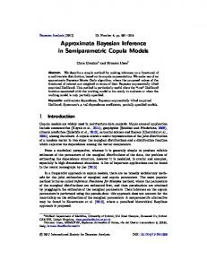
For example, F igure 1 shows both densities f ) and where f is the density of P and the den sity of the contribution to the total probability mass Now of instantiations with associated probability 50 %of the instantiations, i.e., instantiations with as sociated probability P > 10, contribute 98.8 % to the total probability mass (the area below the function in the region P > 10). Consequently, consideration of only these instantiations leads to a maximum error of 0.012 in any probability evaluation.
g(p),
(p)
g(p)
p.
g
P(V).
P(V).jp) og ; 0 � p �A
i
=
p 2 (1 + 2 log (A / p)). A2
'
0
0.02
(24)
0< - A - p< (25)
Figure 5 shows f ( p) and the normalized g( p), which is the pdf associated with G( p),for A 1 . From this we can find that 32% of the instantiations contribute 0.05% of the total probability.
G+
=
(;0
0.0008
(23)
p
J0 g( p)d p
0.01
(22)
�P �A.
with cdf
G+ (;
0.01
j 0.05
(21)
A
0.001
q-+
f (p)
,g(p)
Figure 3: Accumulated probability, exact and approximate values with
u =
0.001 for network with probability tables
selected from [0,0.1] U [0.9,1].
consider the Bayesian belief network (Bs,Bp) in Fig ure 4. Then, we have P = f(xl)f(x2lxl)f(x31xl), so X3< x1. P =Aexp(-Axl)exp(-xlx2); x1,x2 >0, 0 < ( 19 ) 1
-Ax 1
f(x1)=J.e
;
x 1 >0 -x1x 2 f(x2 1x1)=x1e ; x2>0
f(x31x1)=1/x1;
Figure 4:
First we consider the change of variable: U=X1
f(p),
and normalized
g(p)
functions.
We can simulate (X1, X2,X3) using the conditional probabilities in Figure 4. We have simulated a sample of size 1000, which is shown in Figure 6.
Example of a Bayesian belief network.
P =A exp (-X1(A + X2))
Figure 5:
O