fields of repeat-pass SAR interferometry and SAR image focusing. Important .... In the above, H represents the satellite height above the reference surface, B the ..... The unwrapped interferometric phase is assumed to be composed of the following terms: ( , ) topo disp base atmo ..... indicated with Ï and its units shall be m.
ERROR MODELLING FOR SAR INTERFEROMETRY AND SIGNAL PROCESSING ISSUES RELATED TO THE USE OF AN ENCODING SAR TRANSPONDER Ph.D. thesis John Peter Merryman Boncori
2006
Supervisor: Prof. Giovanni Schiavon
Faculty of Engineering, Department of Computer Science, Systems and Production, Geoinformation Ph.D. Programme, University of Rome “Tor Vergata”
2
Contents Acknowledgements ................................................................................................. 5 Introduction ...........................................................................................................
6
1
8
Interferometry background ........................................................................... 1.1 Interferometric phase 1.2 Height measurement from a single interferogram 1.3 Overview of error sources
2
Current error estimation and correction techniques ................................... 13 2.1 Introduction 2.2 Single-interferogram techniques 2.2.1 Phase decorrelation 2.2.2 Orbit indetermination 2.2.3 Atmospheric propagation 2.2.4 Phase unwrapping errors 2.3 Multi-interferogram techniques 2.3.1 Terrain elevation 2.3.2 Terrain displacement
3 Proposed error prediction framework ........................................................... 19 3.1 Introduction 3.2 Height errors 3.2.1 Notation and problem statement 3.2.2 Baseline calibration 3.2.3 Calibrated path-length uncertainty 3.2.4 Phase unwrapping errors 4 Atmospheric error modelling .......................................................................... 24 4.1 Physical causes for atmospheric artefacts in SAR interferograms 4.2 Statistical modelling approaches 4.2.1 Refractivity and delay structure functions 4.2.2 Power spectral density of phase artifacts 4.3 Proposed model 4.3.1 Modelling objectives 4.3.2 Mathematical formulation 4.3.3 Mathematical derivation 4.3.4 Convergence at infinity and parameter L 4.3.5 Computation of P0 and L parameters 4.3.6 Tests for the choice of the best approximation for the structure function 4.4 Conclusions
3 5 Phase unwrapping error modelling ............................................................... 44 5.1 5.2 5.3 5.3
Problem statement Local error indicators Global error indicators Proposed model 5.4.1 Underlying Assumptions 5.4.2 Single cut model 5.4.3 Generalization to the multiple cut case 5.4.4 Closed forms for the structure function of phase unwrapping errors
6 Application to DEM generation: the Castelli Romani data set ................... 53 6.1 Data set overview 6.2 Castelli i7 interferogram 6.2.1 Observed DEM errors and predicted accuracy, based on coherence, GCP height accuracy and atmosphere 6.2.2 Evidence of phase unwrapping errors 6.2.3 Inclusion of phase unwrapping error modelling in the error prediction 6.3 Castelli i4 interferogram 6.4 Castelli i5 interferogram 6.5 Castelli i6 interferogram 6.6 Conclusions 7 Signal processing issues related to the exploitation of an encoding SAR transponder ............................................................................................ 70 7.1 Introduction 7.2 Working principle and previous studies 7.3 Problem statement 7.3.1 Device impulse response 7.3.2 Azimuth frequency domain 7.3.3 Code synchronization 7.4 Proposed processing algorithm based on time domain correlation 7.5 Transponder signal properties 7.5.1 Characteristics of the focused signal 7.5.2 Characteristics of the defocused signal 7.6 Transponder performance in a random scene 7.6.1 Signal decoupling - analytical modelling 7.6.2 Code synchronization and PBR loss - analytical modelling and simulations in a homogeneous scene 7.6.3 Effects of a non-homogeneous scene - generalization of the results and simulations in an urban environment 7.7 Real data processing - DLR prototypes 7.8 Conclusions
4 8
Conclusions ..................................................................................................... 8.1 8.2 8.3 8.4
91
Overview Atmospheric error modelling Phase unwrapping error modelling Encoding transponder signal processing
Appendix A Encoding SAR transponder signal decoupling: analytical modelling derivations ...............................................................….……………… 95 References .........................................................................................................… 100
5
Acknowledgements The work reported in this thesis was carried out in more than one institution. It all started in October 2002 when I was assigned a graduation thesis on an encoding SAR transponder at ESA/ESRIN in Frascati (Rome), under the supervision of Pier Giorgio Marchetti, ESA. The work carried out on this subject after my enrolment in November 2003 in the Geoinformation PhD programme at the University of Rome "Tor Vergata", has been a continuation of the one started during my graduation thesis. My first thanks goes to Pier Giorgio, for involuntarily starting a chain of positive encounters and events in my life as well as for his voluntary and ongoing support and advice. Secondly I wish to thank my University advisors, Prof. Domenico Solimini and Prof. Giovanni Schiavon for their support throughout my PhD. Had they not provided funding for exotic (at least from an Italian point of view) IGARSS venues such as Anchorage and Seoul, as well as for EUSAR conferences, contacts and cooperation with Prof. Dr. Alberto Moreira, Dr. D. David Hounam and Dr. Marco Schwerdt, Institut für Hochfrequenztechnik, DLR, would likely never had happened, as well as the much appreciated discussions with Brian Barber, DSTL, on SAR processing issues and Dinesh Manandhar, University of Tokyo, concerning GPS code acquisition techniques. Thanks to DLR members for providing the encoding transponder data set used for validating the focusing algorithm, and thanks for Mr. Barber and to Dinesh for the time spent answering my questions. Since January 2006 my PhD was carried out visiting Denmark's Technical University, EMI department, under the supervision of Prof. Johan Jacob Mohr. Here the work concerning SAR interferometry was carried out. A special thanks goes to Johan for all the time spent teaching me new things, for his generous support and advice, tak for det!
6
Introduction The broad context of this work is that of Synthetic Aperture Radar (SAR) data processing for the measurement of geophysical parameters. More specifically, theoretical and experimental work has been carried out throughout the thesis in the fields of repeat-pass SAR interferometry and SAR image focusing. Important applications of repeat-pass SAR interferometry in the last decade have been the measurement of topographic height and surface displacement (or equivalently velocity). Error estimation is required in all quantitative applications, yet to a significant extent it may still be considered an open research field, particularly for applications in which a minimum data set may or must be exploited. Two of the most relevant error sources are space-time fluctuations of the atmospheric refractive index and phase unwrapping errors. Their statistical modelling forms a central part in this thesis and is of interest for various purposes, given the current state of the art. Firstly, for Digital Elevation Models (DEMs) and displacement maps generated using a minimum number of interferograms, a standard approach to assess the accuracy of the derived geophysical products does not exist to date. A framework meant for this purpose has been recently proposed [Mohr2006a], and relies on models for the second order statistics of the non-deterministic error sources. Secondly, within multi-interferogram frameworks, although it has been proved that a high degree of accuracy may be achieved, a procedure to provide a confidence measure for each pixel, which accounts for atmospheric as well as phase unwrapping errors has not been published to date. As far as DEM generation is concerned, either only atmospheric errors are accounted for, but phase unwrapping ones are not [Ferretti1999], [Allievi2001], or phase unwrapping is avoided, but atmosphere (spatially correlated error sources) may not be accounted for [Eineder2005]. As far as displacement (and DEM refinement) is concerned, unwrapping errors are typically assumed to be negligible and atmospheric errors are handled in a sub-optimal way in order to simplify the processing [Ferretti2000], [Berardino2002], [Mora2003]. Within these processing schemes, simple closed forms for the second order statistics of the main error sources might be useful in the future to improve data processing as well as accuracy assessment. Finally, some recent studies have addressed the problem of atmospheric error correction, using systems other than SAR, namely GPS [Williams et al., 1998] and satellite imaging spectrometers [Moisseev2003], [Li2005], [Li2006a]. These studies elicit interest for statistical error modelling, since external measurements are typically available on a sparse grid compared to interferometric SAR measurements, so that some form of interpolation is required. Preliminary results indicate statistical interpolators to be the most effective for this task and these typically exploit models of the second order statistics of the error source. In Chapters 4 and 5 of this thesis, errors due to atmospheric propagation and phase unwrapping respectively are discussed in detail and a model for the second order statistics of each is derived. In Chapter 3 a framework is presented, which exploits such models to obtain a confidence measure for each pixel for height maps created with a minimum number of interferograms. This is the result of the work of Prof. J.J. Mohr, at Denmark’s Technical University (DTU), Electromagnetic department (EMI). At the time of writing, an extension of the model to displacement measurements is a subject of undergoing work.
7 A preliminary validation of the error estimation framework and of the models is described in Chapter 6 for DEM generation from ERS-tandem acquisitions. The causes of some apparent artefacts and the performance of the error prediction models are discussed in detail, using an external SRTM DEM as a reference. Alongside error modelling, this thesis also addresses SAR signal processing issues related to the use of a specific class of artificial reflectors. In the context of SAR interferometry, these have been used as tie-points for accurate geocoding and refinement of orbital data [Gutjahr2005] or as stable reflectors in the framework of persistent scatterer methodologies [Allievi2004]. Typically passive reflectors (Corner Reflectors) have been exploited for these purposes. Active ones however, i.e. SAR transponders, may offer advantages compared to CRs, such as reduced size for a specified RCS (particularly in L band), cost-effectiveness and ease of installation. Furthermore, active devices offer the possibility of superimposing a modulation on the SAR signal, which may be used to increase the signal decoupling with respect to natural backscattering [Shimada99], [Weiss2004] and/or for automatic location and identification [Hounam2001] of the device. These benefits are basically paid for by adding complexity to the design of the transponder’s electronics and antenna(s) as well as to the SAR data processing algorithm. In Chapter 7 of this thesis a specific SAR transponder architecture is considered, namely a pulse-to-pulse encoding SAR transponder patented by a research group at DLR [Hounam1998], [Hounam2001]. The existing literature focuses on device architecture, working principle demonstration and potential applications, rather than on data processing issues. In this thesis, issues related to the SAR focusing algorithm, to the code alignment procedure as well as to transponder signal decoupling compared to natural backscattering are discussed. Equations are derived which allow for tradeoffs between processing efficiency, device Radar Cross Section (RCS) and detection probability. Theoretical derivations are validated through point scatterer simulations and through the processing of an ERS data set containing transponder prototypes developed at DLR. The approach followed in carrying out these investigations was intentionally not restricted to SAR interferometry or to any other specific application. The results obtained may rather be of interest for more than one proposed application, including SAR interferometry.
8
Chapter 1
Interferometry Background 1.1 Interferometric phase Interferometric SAR techniques have been the subject of several review articles [Bamler1998], [Massonnet1998], [Rosen2000] and books [Ghiglia1998], [Hannsen2001]. This section serves the purpose of establishing notation and recalling results useful for further discussions. The material presented in the following is based on the above works as well as on published works with particularly clear recapitulations, namely [Zebker1994a], [Joughin1996] and [Hannsen1998a]. Since the focus throughout this thesis is error analysis, the flat earth and parallel ray approximations shall be made in all equations where needed, a procedure which retains sufficient accuracy for the purpose of error analysis. Furthermore, a repeat-pass interferometric configuration shall be assumed. Considering the two SAR images forming an interferometric pair, the complex pixel value in each may be written as:
V1 = exp ( − j 2kr1 ) W1 = exp ( − j 2kr1 ) exp ( −2k ∆re1 ) A1e jφ1 V2 = exp ( − j 2kr2 ) W2 = exp ( − j 2kr2 ) exp ( −2k ∆re 2 ) A2 e jφ2
(1.1)
where k = 2π/λ is the wave number, λ the radar wave length, ri the slant range distance to the pixel in image i, ∆rei represents an excess path-length due to atmospheric propagation at acquisition time i and Wi shall be assumed a complex, circular Gaussian random variable. The former models various sources of decorrelation between the backscattered phase at the two acquisition times [Zebker1992]. The phase of an interferogram pixel is then: arg(V1V2* ) = ⎡⎣ −2k ( r1 − r2 ) − 2k ( ∆re1 − ∆re 2 ) + (φ1 − φ2 ) ⎤⎦ mod(2π )
(1.2)
The first term on (1.2) is the one of interest for height and displacement measurements, the remaining terms and the fact that phase values may be observed only in the [0, 2π) interval are considered disturbances for these applications.
9 Phases φ1 and φ2 are uniformly distributed in [0, 2π), however provided W1 and W2 are highly correlated, the difference (φ1-φ2) is sharply peaked around a zero mean value [Bamler1998]. A second error term is due to atmospheric delay, a discussion of which shall be postponed to chapter 4 of this work. At this point it is merely of interest to state that in general this contribution may not be neglected. Finally, all phase values in the interferogram are observed in the interval [0, 2π), and an unwrapping algorithm is used to derive the correct phase differences between pixels. The unwrapping procedure itself is carried out from a certain starting point in the image, thus providing the absolute phase only up to an unknown constant. This in turn may be determined either from one or more reference points of known elevation (tie-points) or from the radar data itself [Rosen2000]. In this work the former approach shall be followed (see chapter 3), and for the present discussion it shall be assumed the unwrapped phase has been compensated for this ambiguity. In the following two paragraphs, equations relating the unwrapped interferometric phase to the geophysical parameters of interest for this work shall be derived, assuming no error sources are present. An overview of these shall be provided in paragraph 1.4, postponing a detailed discussion to further chapters of this thesis.
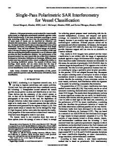
1.2 Height measurement from a single interferogram From the geometry in Fig. 1, assuming a flat earth, and no displacement between the two acquisitions, height above a reference surface may be computed solving the following equations for the radar look angle θ and topographic height h [Zebker1994a]:
φunw = −
4π
λ
B sin (θ − α )
(1.3)
h = H − r1 cos θ
In the above, H represents the satellite height above the reference surface, B the interferometric baseline, and α its orientation angle. These quantities may be derived from the satellite state vectors, and in the present discussion it is assumed these aren't affected by any error. Finally r1 represents the slant range measured from satellite 1, which is obtained from the SAR image control data fields. For convenience in following discussions, it shall be useful to solve (1.3) by introducing the flat earth contribution to the unwrapped interferometric phase, which shall be referred to in the following as "flattening phase" and is given by (1.4).
φ flat = −
4π
λ
B sin (θ 0 − α )
(1.4)
In the above θ0 represents the look angle for each point in the image, assuming zero local height.
10 2 B α
1
B|| B⊥ r2
θ r1
H
h Fig. 1 Interferometer geometry
Subtracting this contribution yields the unwrapped topographic phase (1.5), which may be related to the sought height through known terms.
φtopo = φunw − φ flat � −
4π
λ
(θ − θ 0 ) B cos (θ 0 − α ) = −
4π B cos (θ 0 − α ) h λ r1 sin θ 0
(1.5)
In (1.5) the last equality follows by differentiating both sides of (1.3). Throughout this thesis reference shall be made to the parallel and perpendicular components of the baseline, which are depicted in Fig. 1 and defined as follows B& = B sin (θ − α ) � r1 − r2
(1.6)
B⊥ = B cos (θ − α )
(1.7)
These are signed values, and their sign is defined implicitly by the choice of the orientation angle α, [Hanssen2001]. In the present work this angle shall be chosen to be positive counter-clockwise, starting from the reference satellite 1, as for the look angle θ. With this choice B⊥ will be positive whenever satellite 2 is located to the right of the slant range of satellite 1 and in this case B|| will increase from near to slant range and from foot to top of a mountain. Having defined these quantities, the unwrapped topographic phase may conveniently be rewritten as:
φtopo = −
4π
B⊥,θ0
λ r1 sin θ 0
h
(1.8)
In the above B⊥,θ0 represents the perpendicular baseline component for each point in the image, assuming zero local height.
11 For further discussions, it shall finally be useful to consider also the variations in the unwrapped interferogram phase (∆φunw) in the error free case. In the absence of surface motion, contributions are due to slant range variations (∆r) at a constant height and to height variations (∆h) at a constant slant range. These effects shall be considered to be decoupled throughout this thesis, such that:
∆φunw = ∆φ flat + ∆φtopo
(1.9)
It may be proved that the following equations hold for the terms on the right hand side of (1.9):
∆φ flat =
4π B⊥,θ0 ∆r ⋅ λ ⋅ r1 tan θ 0
(1.10)
∆φtopo =
4π B⊥,θ0 ∆h ⋅ λ ⋅ r1 sin θ 0
(1.11)
1.3 Overview of error sources Accuracy in height and displacement (or velocity) measurements is known to be affected by orbit indetermination (baseline errors), scattering decorrelation (phase noise), atmospheric propagation and phase unwrapping errors. Baseline values must be derived for each interferogram pixel, based on orbital data. Errors are mainly due to radial and across track satellite positioning errors. These in turn cause an error in the flat-earth phase (1.4) as well as in the phase-to-height (1.8) conversion factor. The first is predominant for ERS interferometry. For a fixed azimuth position, the error in the flat-earth phase is well approximated by a parabolic (almost linear) function of slant range. For ERS interferometry, this may cause a phase gradient ranging between 0 to 1 phase cycles across the whole interferogram [Hanssen2001]. In the along track dimension, baseline varies linearly in time during image acquisition due to track convergence. Phase noise is due to various error sources, including processing artefacts [Just1994], thermal noise, geometric and temporal decorrelation [Zebker1992]. Thermal noise depends on the radar electronics and for the current systems it becomes significant only on areas of low backscatter. Geometrical (or baseline) decorrelation is due to the finite resolution cell of the radar, which causes the phase value of each pixel to be determined by a coherent sum of contributions from elementary scatterers (of wavelength size) in each cell. As interferometric baseline increases this coherent sum will be increasingly decorrelated in each acquisition geometry, eventually reaching zero for the so called “critical” baseline value. Finally, temporal decorrelation refers to changes in scatterer properties between the two acquisition times. All these decorrelation error sources are weakly correlated from pixel to pixel, or equivalently their power spectrum is broadband. Atmospheric errors are due to spatial variations of the atmosphere’s refractive index, which alter the phase (and group) velocity of the electromagnetic wave. They have received much attention in the last decade, due to their order of magnitude, which may amount up to several phase cycles at C band [Hanssen2001]. Such variations
12 occur on a wide range of spatial scales, from hundreds of meters to thousands of kilometres, causing the phase bias in (1.2) to be inhomogeneous within the interferogram and the artefacts to have a strong spatial correlation. Phase unwrapping errors are caused by and the presence of phase gradients between adjacent pixels exceeding π in magnitude. In turn these are due to phase noise and radar shadow, to phase under-sampling induced by steep topography and phase noise as well as by discontinuous surface deformation and by radar layover. Errors arise in the integration of phase gradients, which can lead to local as well as large-scale errors due to error propagation.
13
Chapter 2
Current Error Estimation and Correction Techniques 2.1. Introduction A common objective of all interferometric processing schemes is to distinguish the contributions due to the geophysical signals of interest from those due to the error sources mentioned in paragraph 1.4. In the literature of the last decade, several researches have addressed the single error sources, mainly in the context of height and displacement measurements from one or two interferograms. Multi-interferogram processing schemes have been proposed more recently, which exploit the greater amount of available data not only to achieve better accuracies in the derived geophysical measures, but also to improve error estimation. This section aims at summarizing the results of these studies regarding the latter purpose. As far as singleinterferogram techniques are concerned, this section shall report only the results of the main studies, whereas a more detailed discussion on error modelling and characterization may be found in chapter 3, chapter 4 and chapter 5, which deal specifically with baseline calibration, atmospheric and phase unwrapping errors respectively.
2.2. Single-interferogram techniques 2.2.1 Phase decorrelation The phase variance of each interferogram pixel due to this error source is generally computed from the local magnitude of the coherence, γ . The latter is defined as the complex correlation coefficient between pixel values in the images forming the interferometric pair [Rodriguez1992], [Zebker1992]. This parameter is in turn estimated through a spatial average around each considered pixel, assuming the processes which contribute to phase noise to be ergodic and stationary within the estimation window [Bamler1998]. It has been observed that this estimate is a biased one for low coherence values, and approaches to obtain unbiased estimates have been proposed [Touzi1999]. Equations relating the probability density function of the
14 observed interferometric phase around its expected value, in the presence of decorrelation, have been published [Just1994], [Eineder2005]. These are a function of coherence and of the number of “looks” L, i.e. the number of samples averaged in the estimate. Evaluation of these expressions to derive the phase variance involves special functions so that the Cramer-Rao bound for the phase variance (2.1) is often used. It has been proved to be accurate enough, provided more than four looks are taken [Rodriguez1992]. 1 (1 − γ σφ = 2L γ 2 2
2
)
(2.1)
In order to reduce the phase variance due to phase noise, many processing schemes implement a fringe-rate filtering technique proposed in [Goldstein1998], a refinement of which is proposed in [Baran2003]. This method performs an adaptive band-pass filtering of the fringe-rate, dφ/dr, in the frequency domain, relying on the wide bandwidth of the processes contributing to phase noise compared to the fringe rate variations due to slant range and terrain slope. As far as error estimation is concerned, the impact of this filtering on the properties of the remaining error sources, has not been assessed to date.
2.2.2 Orbit indetermination Several authors have proposed a tie-point approach to refine the orbital data and “calibrate” the interferometric baseline [Werner1993], [Small1993], [Zebker1994]. This procedure relies on the availability of a set of points of known height in the image and on a baseline error model. One choice for the former may be a physical model, which typically accounts for the along track convergence of the orbits through a linear variation of two baseline vector components with the along-track coordinate [Small1993], [Joughin1996], [Costantini2001]. Baseline models which account directly for the induced phase or path length error in the interferogram have also been proposed [Zebker1994], [Hubig2000], [Mohr2003]. Using the tie-points, a system of equations may be formed, as detailed in chapter 3 of the present work, and solved in a least-square sense for the parameters which describe the baseline model. Estimation of the absolute phase constant may be carried simultaneously [Small1993]. Improved implementations of the tie-point strategy, in the face of phase unwrapping errors have been proposed [Hubig2000], [Costantini2001]. Furthermore, the simulations presented in [Zebker1994] and [Joughin1996], have shown that the robustness of tie-point methods strongly depend on the spatial configuration and number of the control points. Other authors have argued that the effects of atmospheric and phase unwrapping errors on this procedure are anyhow not easily predictable, and that baseline calibration is more safely performed by removing a phase bias and a slope (or second order polynomial) from the interferogram [Hanssen2001]. A trend-removal approach known as “artificial baseline” correction is also proposed in [Tarayre1996] and [Massonnet1998]. The baseline is corrected by observing the phase difference crossing the interferogram from near to far range and adjusting the slave satellite position accordingly. It is argued in [Hanssen2001] that this procedure is effective
15 only for the parallel component of baseline error (which leads to flattening error), and may potentially worsen the error in the perpendicular component. It has been pointed out however that the trend-removal approaches may have hardly predictable consequences on the statistical properties of atmospheric error sources, thereby complicating their estimation and/or correction during further processing steps [Williams1998].
2.2.3 Atmospheric propagation Since atmospheric artefacts were first observed in interferograms [Massonnet1995a], [Massonnet1995b], [Goldstein1995], [Zebker1997], efforts have been devoted to their statistical characterization and reduction. Several recently proposed statistical modelling approaches have drawn upon experiences within the radio wave propagation community and Kolmogorov turbulence theory [Tatarski1961]. Accordingly, the main effects on propagation are due to fluctuations in the water vapour concentration, which are believed to occur at many different scales. The magnitude of the disturbances exhibits a power law spectral density. A significant correlation is likely to be present at distances of several kilometers, which also implies that the spatially estimated correlation γ may be high also in the presence of strong atmospheric errors. Basically the ergodicity hypothesis falls and a real ensemble average would be needed in order to capture the atmospheric error contribution through γ. This is not possible in a single-interferogram framework Recent studies have related GPS (Global Positioning System) and VLBI (Very Large Basline Interferometry) observations and modelling techniques to SAR interferometry. In [Williams1998] a covariance matrix for tropospheric delays in a SAR interferogram is proposed, based on a model originally proposed for VLBI applications, [Treauhaft and Lanyi, 1987]. This in turn draws upon Kolmogorov turbulence theory [Tatrski1961], for description of the second order statistics of refractivity variations. In [Hanssen1998a] and [Hanssen2001], an extensive comparison between InSAR (Interferometric SAR) observations of atmospheric artefacts and meteorological data is carried out. Based on this, a power spectral density model is proposed for the neutral atmospheric delay, drawing upon turbulence theory. The model requires a free parameter to be initiated in order to provide a correct statistical description of the artefacts affecting a specific data set. A statistical approach was adopted to this end in [Hanssen2003], whereas available microwave radiometer measurements were used in [Moisseev2002]. Due to the reduced topography of the data set examined in [Hanssen1998a], the effects of topography-correlated artefacts, due to changes in the vertical stratification of the refractive index at the two acquisition times, was not examined in this study. However an empirical model for the phase standard deviation due to this error source is proposed in [Hanssen2001], based on radiosonde profiles of atmospheric parameters. As far as atmospheric error correction is concerned, current researches address the use of GPS Zenith Neutral atmosphere Delay (ZND) measurements as well as imaging spectrometer data (NASA-MODIS, ESA-MERIS). Calibration using ZND measurements was first proposed in [Williams1998]. Due to the sparse grid (GPS network) on which such data is available, an interpolation is
16 required to apply any correction to a SAR interferogram. Statistical interpolators, based on the second order statistics of atmospheric excess delay, are expected to be the most suitable according to [Williams1998]. A statistical model has been recently proposed for this purpose in [Li2006], which accounts also for topography-correlated atmospheric artefacts. A similar model was derived in [Emardson2003], based on GPS measurements, in order to estimate the accuracy of an interferometric SAR stack for surface deformation rate measurements. Feasibility studies and first results have been recently carried out, concerning correction of tropospheric water vapour fluctuations using Spectrometers [Moisseev2003], [Li2005], [Li2006]. The first results highlight the importance of these measurements to be synoptic with SAR acquisition as well as that of the interpolation method used to extend the measurements from the resolution of current imaging spectrometers (300 m for MERIS, 1 km for MODIS) to the finer SAR resolutions (40 m to 100 m for ERS interferograms).
2.2.4 Phase unwrapping errors While a wealth of literature exists regarding phase unwrapping algorithms and causes of phase unwrapping errors are also reported and discussed in several papers, reviewed in chapter 5 of the present work, very few explicitly address characterisation and/or correction of phase unwrapping errors. A procedure based on a segmentation map, formed from residue density thresholding was presented in [Hubig2000] to automatically correct for baseline and PU errors. Pixels exceeding a certain residue density threshold and those exhibiting a phase jump greater than π with one of their neighbours are masked out. The non-masked out pixels are divided into connected regions, allegedly the consistently unwrapped ones. A least square fit of available tie points is then performed in each region to estimate the baseline. The best estimation strategy was found to be a four-parameter estimate in the largest connected region and just a bias estimate in all the others. In this way calibration effectively removes also large-scale PU errors, providing the regions of consistently unwrapped phase were correctly identified. To this end, the method is proved to be very sensitive to the residue density threshold value, although conservative thresholds may anyhow be set at the price of a greater percentage of masked out regions. In [Galli2001], an algorithm based on a Maximum Capacity Path (MCP) index is presented, which allows location of PU errors and potentially also correction of large scale ones. The algorithm relies on a confidence map, a measure of phase quality, which in the author’s tests is a correlation coefficient magnitude map, although in principle also amplitude and wrapped phase information could be combined. To each arc connecting neighbouring pixels a capacity is associated based on this map, low capacity meaning low quality data. A reference pixel is chosen arbitrarily and the path crossing the highest quality data, i.e. the one with maximum capacity, is chosen from each pixel to the reference one. The capacity of such a path is referred to as the MCP index of that pixel, a measure of how well each pixel is connected to the reference one. The computation of this index for each pixel creates a connectivity map, in which problematic areas should be recognizable. A threshold on the MCP index may then be used to mask out unreliably unwrapped regions, and Ground Control Points (GCPs), when available, may be used to try and correct for large-scale errors.
17 In [Suchandt 2003] the quality assessment strategies used for the processing of SRTM/X-SAR data are briefly described. Three tools were used to guide operating personal in identifying scenes with problematic PU: the above mentioned segmentation procedure [Hubig2000], a comparison with a synthetic interferogram generated from an external DEM, and an automatically generated map of allegedly wrong branch cuts. The latter was created based on cut length, and on a comparison between the costs associated to the cut by the used MCF implementation and the wrapped phase gradients across the cut. Also in other papers, including the already mentioned [Hubig2000], [Galli2001] and [Suchandt2003], a synthetic interferogram from an external DEM is exploited. The difference image of the unwrapped phase and the synthetic one is visually inspected, for example in [Chen2001] and [Chen2000], while an analysis of its pdf has also been used to assess the level of agreement of the two data sets in [Hubig2000]. Also coarse resolution DEMs, on the order of 1 km, proved to be useful for this kind of quality check [Suchandt2003], [Hubig2000]. Finally, phase unwrapping reliability is discussed in the context of region growing algorithms, such as [Chen 2002] and references therein, although in these studies the presented methodologies are aimed at performing the unwrapping, avoiding error propagation rather than estimating the error of an unwrapped field.
2.3 Multi-interferogram techniques 2.3.1 Terrain elevation As far as the generation of Digital Elevation Models (DEMs) is concerned, a method has been proposed [Ferretti1999], which exploits multiple interferograms and wavelet transforms to separate the contribution of an error source with a power law spectral density, i.e atmosphere, from other error contributions. This has first of all the effect of allowing proper weighting coefficients to be derived, in order to carry out a weighted average of the DEMs obtained from each interferometric pair. Secondly it allows the error variance to be estimated for each pixel. The procedure assumes orbit errors have been estimated and requires unwrapped interferograms, which potentially may contain errors which are unaccounted for. A strategy to exploit a multiple interferogram data set for phase unwrapping and baseline estimation has also been proposed in literature [Ferretti1996], [Ferretti1997]. An algorithm which combines this procedure with the above described wavelet based weighting scheme was presented in [Allevi2001] and has been proved to give robust results using 6 to 8 ERS tandem interferograms. Ultimately it provides a pixel error variance estimate, which accounts for all main error sources except for a final phase unwrapping step. Potentially however, phase undersampling problems are strongly reduced compared to the single-interferogram case, provided the baseline configuration is favorable. This is achieved by obtaining a coarse topography by locally applying a Maximum Likelihood (ML) approach. This in turn is based on the unwrapped phase gradients and on statistical models for their probability density functions, for a given height difference, interferogram geometry, amplitude and coherence. Subtracting the contribution of this coarse topography to each interferogram is expected to strongly reduce the number of phase residues, easing the task of conventional phase unwrapping algorithms. Baseline errors are estimated from the unwrapped phase, by a local least-mean-squares estimate, either using points of
18 known height (tie-points) or by comparing to the ML height estimate derived from the largest baseline interferogram. A multi-interferogram DEM generation algorithm, which exploits a similar ML approach as in [Ferretti1996], is described in [Eineder2005]. This methodology differs though, in that it does not require phase-gradient computation to carry out phase unwrapping. Furthermore the information coming from the single interferometric pairs is combined in the height domain, allowing for exploitation of satellite passes with different viewing geometries, as well as low resolution DEMs. However atmospheric artefacts, and in general spatially correlated ones, may not be accounted for and the error variances derived therefore do not account for this error source.
2.3.2 Terrain displacement As far as displacement in general is concerned, two classes of multi-interferogram processing schemes have been proposed, which, assuming an initial DEM of the area of interest is available, are able to provide a displacement measurement as well as an atmospheric error estimate and a refinement of the initial DEM. The first class comprises the original Permanent Scatter (PS) technique developed within the Politecnico di Milano research group [Ferretti2000], [Ferretti2001], [Colesanti2003] as well as other "Persistent Scatter" algorithms which share the same basic principles (see [Hooper2004] and references therein). The second class comprises the Small BAseline Subset algorithm (SBAS) algorithm [Berardino2002] and the Coherent Pixels Technique (CPT) [Mora2003]. For the present discussion it is just of interest to note that both classes of algorithms isolate atmospheric components using a spatio-temporal filtering, relying on the poor temporal decorrelation of this error source compared to motion components and on its longer spatial correlation length compared to non-linear displacement. Moreover baseline errors are treated as long-wavelength atmospheric errors (smoothly varying throughout the image) in both classes of algorithms. Finally phase unwrapping is carried out using a multi-image approach, in which the major contributions to critical phase gradients, namely topography and linear motion components, may be estimated and removed prior to this processing step.
19
Chapter 3
Proposed Error Prediction Framework 3.1 Introduction This section summarizes an error prediction framework recently submitted for publication [Mohr2006a]. It is the result of work carried out by Prof. Johan Mohr at Denmark’s Technical University, Electromagnetics department (EMI). The problem addressed is the estimation of the variance of height measurements obtained from a single interferometric pair. It is assumed a set of Ground Control Points (GCPs) are available, of known height and position. Separation of the contribution of the various error sources from that of terrain topography is formulated as a least-square estimation problem in the presence of coloured noise. The goal is to estimate a constant path length (or equivalently phase) bias and higher order coefficients of a baseline error model, by computing a least-mean-square fit to the observed path length error at each GCP. The estimation procedure assumes the mean error on the observables is zero and requires knowledge of the variance-covariance matrix of the error affecting the GCPs. In order then to predict the phase variance of an interferogram pixel after it has been calibrated by the estimated baseline, it is also required to know the variance of the error affecting each pixel of interest and the covariance between the error affecting each pixel of interest and each GCP. The required statistics may be derived through error models for each error source, which shall be the objective of chapters 4 and 5 as far as tropospheric delay and phase unwrapping errors are concerned respectively.
3.2 Height errors 3.2.1 Notation and problem statement The unwrapped interferometric phase is assumed to be composed of the following terms:
ϕ ( x, y ) = ϕtopo + ϕ disp + ϕbase + ϕ atmo + ϕ noise + ϕunw
(3.1)
20 which are all functions of the SAR image coordinates (x,y). The terms are due respectively to terrain topography, terrain displacement, baseline error, atmospheric delay, phase noise and unwrapping error. In the following φbase shall represent only flattening errors caused by a wrong baseline value, and it will be supposed φtopo can be calculated if the elevation is known (see paragraph 1.2). In the following the observable shall be considered the slant range difference, δ, referred to as “interferometric path-length”. For a repeat-pass interferometer it is related to φ by:
δ =−
λ ϕ 4π
(3.2)
An error in interferometric path length translates to an error in the inferred height through the following linear relation (see equation 1.8), sufficiently accurate for error analysis:
σh =
R sin θ σ δ ,topo B⊥
(3.3)
R represents slant range, θ and B⊥ are respectively the radar incidence angle and the perpendicular baseline value assuming zero height, σδ and σh represent the standard deviation of interferometric path length and elevation respectively. Displacement error in the radar line-of-sight direction is simply
σ d = σ δ ,disp
(3.4)
where σd denotes the standard deviation of the line-of-sight displacement. For error analysis, the following terms are of interest:
δ ( x, y ) = δ base + δ atmo + δ noise + δ unw
(3.5)
Any deviations of δ(x,y) from zero translate into geophysical measurement errors through (3.4) and (3.5). 3.2.2 Baseline calibration
The effects of baseline errors on the flattening phase are well approximated by a path length of the form [Mohr2003],
δ base ( x, y ) = b1 + b2 x + b3 y + b4 xy = p⋅b
(3.6)
where p = [1,x,y,xy]´, b = [b1,b2,b3,b4]´, x is the along-track coordinate, y is the across–track coordinate, and bi the coefficients to be estimated through the baseline calibration procedure. If GCPs of known horizontal position, height and displacement (usually equal to zero) are available, their expected path length contributions may be subtracted from the
21 observed values. The resulting interferometric path length, δobs, observed at the GCP positions is then given by
δ ( x, y ) = δ base + (δ atmo + δ noise + δ unw + δ gcp )
(3.7)
The first term on the right hand side is the deterministic baseline error given in (3.6). The remaining error terms are realizations of zero mean stochastic processes and there mean is assumed to be zero. The last term on the right accounts for errors in the horizontal position, height and displacement of the GCP and its variance shall be denoted by σ2gcp. All path-length biases are contained in the b1 parameter in (3.6). This term shall also comprise an absolute phase constant and the average atmospheric delay between the two acquisitions. Assuming the error terms mutually independent and normally distributed, the leastsquare estimation problem for N GCPs may be written as
y = Xb + ε
(3.8a)
y = [δ1 ,...., δ N ]´
(3.8b)
where
⎛1 x1 ⎜ # # X =⎜ ⎜# # ⎜⎜ ⎝ 1 xN
y1 # # yN
x1 y1 ⎞ ⎟ # ⎟ # ⎟ ⎟ xN y N ⎟⎠
(3.8c)
ε ∈ N ( 0, Σε )
(3.8d)
Σε = Σatmo + Σnoise + Σunw + Σ gcp
(3.8e)
Variables [δ1,…,δ N], represent the observed GCP path lengths, after subtraction of all known terms. Matrix X depends on the horizontal position of the GCPs. It should be noted that the coordinate system in which these are provided are not important, provided the same choice is made for vector p in (3.6). The matrixes on the right hand side of (3.8e) represent the variance-covariance matrixes of each error term. Two of them shall be considered known, namely Σgcp and Σnoise . These shall be diagonal matrixes with variance σ2gcp and σ2γ respectively. The latter shall be approximated by the following [Rodriguez1992] (cfr. also equation 2.1), ⎛ λ ⎞ 1 (1 − γ σγ = ⎜ ⎟ ⋅ 2 ⎝ 4π ⎠ 2L γ 2
2
2
)
(3.9)
where L represents the number of “looks”, i.e. the number of pixels averaged in the estimation of γ. The least-square solution of (3.8a) is bˆ , given by
22 -1 bˆ = ( X'Σε-1 X ) X'Σε-1 y
(3.10)
= Wy
3.2.3 Calibrated path-length uncertainty The baseline estimate is used to calibrate the observed path length, δp, at a pixel with coordinates (x,y). The calibrated path length, δp*, shall be δp* = δp - p ⋅ bˆ . There will be residual errors after the calibration, due to errors on the observation itself, namely δp,atmo, δp,noise, δp,unw, as well as errors in the calibration term p ⋅ bˆ , which in general will be correlated with δp,atmo, δp,noise, δp,unw, in particularly in the vicinity of GCPs. The variance of the calibrated path length may be written as
{
}
Var {δ p* } = Var δ p − p ⋅ bˆ
= Var {δ p − p ⋅ Wy}
(3.11a)
w p = W'p
(3.11b)
y p = ⎡⎣δ p , −δ1 ,..., −δ N ⎤⎦ '
(3.11c)
y p = N (0, Σp )
(3.11d)
= Var {w p ⋅ y p }
where
−C p , N ⎞ ⎟ ⎟ ⎟ ⎟⎟ ⎠
(3.11e)
2 2 2 V p = Var {δ p } = σ atmo + σ unw + σ noise
(3.11f)
C p ,i = Cov {δ p , δ i } = Catmo (rp ,i ) + Cunw (rp ,i )
(3.11g)
⎛ Vp ⎜ −C p ,1 Σp = ⎜ ⎜ # ⎜⎜ ⎝ −C p , N
rp ,i =
−C p ,1
" Σε
(( x − x ) + ( y − y ) )
2 1/ 2
2
i
p
i
p
(3.11h)
The variance of the single pixel interferometric path-length can then be computed as
σ p2* = w 'p Σp w p
(3.12)
23 Summarizing, the following information is needed to quantify the uncertainty: 1. The positions (horizontal coordinates) of the GCPs 2. The second order spatial statistics (variance and covariance) of the error sources. The second point of this list relies on error models. Two of these are described in chapters 4 and 5 for atmosphere and phase unwrapping errors respectively. In particular modelling efforts should be aimed at computing the following quantities: •
the error variance, Var (δ pi ) , for each point in the image (strictly speaking,
•
only for each pixel of interest and for each GCP). the variance of the error difference, Var (δ pi − δ p j ) , for any pair of points in the image (strictly speaking only the pairs formed between pixels of interest and GCPs are needed).
In fact, the error covariance matrix can be computed from them through the following equation: Cov(δ pi , δ p j ) =
{
}
1 Var (δ pi ) + Var (δ p j ) − Var (δ pi − δ p j ) 2
(3.13)
24
Chapter 4
Atmospheric Error Modelling 4.1 Physical causes for atmospheric artefacts in SAR interferograms Several studies carried out in the last decade have established that SAR interferograms are sensitive to: -
Differences in the horizontal variations of vertically integrated refractivity at the two acquisition times. Differences in the vertical stratification of refractivity at the two acquisition times, between two points at a different height.
Such differences are expected to originate from the radar wave propagation through the different atmospheric layers, particularly troposphere and ionosphere. From the radio propagation scientific community it is well known with that a wave propagating through the atmosphere undergoes bending and propagation delay. For the incidence angles of current remote sensing satellites, the effects of the former on radar interferometry are negligible compared to those of the latter [Hanssen1998a]. Propagation delay is caused by variations of the refractivity, N, along the path between the sensor and the ground, and translates to an excess path length ∆Re measured by the radar. Assuming the wave has travelled through a vertical distance H, this quantity is given by (4.1) [Hanssen1998a, pg. 11]. H
∆Re = 10
-6
N
∫ cosθ
dh
(4.1)
0
In writing (4.1) the defining relation N = 106·(n-1) has been used, where n is the atmospheric refractive index. Excess path length may be expressed in m, or rather in phase cycles referred to a specific radar wavelength. In the following the ERS wavelength of 5.66 cm will be the reference.
25
In turn N is locally related to the total atmospheric pressure (P, in hPa), temperature (T, in K), partial pressure of water vapour (e, in hPa), electron density (ne, per m3), radar frequency (f, in Hz) and liquid water content (W, in g/m3). Many equations have been proposed in literature, for the present work it is chosen to use the following [Hanssen2001, pg. 202] (originally reported in [Davis1985], modified from [Smith and Weintraub 1953]):
N = k1
n P ⎛ e e ⎞ + ⎜ k2 + k3 2 ⎟ − 4.028 ×10⁷ e2 + 1.45W T ⎝ T T ⎠ f
(4.2)
In the above k1 = 77.6 K hPa-1, k2 = 23.36 K hPa-1 and k3 = 3.75 x 10⁵ K2 hPa-1. The values of these constants are reported for completeness, although they shall not be used throughout this thesis. What is important for further discussions is instead to consider the different terms on the right hand side of (4.2). The first causes the so called “hydrostatic delay”, the second term is often referred to as the “wet” component of the refractivity, the third is due to ionosphere and the last accounts for liquid water in clouds. Precipitations also cause a propagation delay but this may be more conveniently treated as a forward scattering problem and modelled as a function of the rainfall rate (see [Moisseev2003] for an application to SAR interferometry). As stated in the bullet list above, SAR interferograms are sensitive to differences in spatial gradients of the excess delay between two acquisitions, rather than to biases affecting a whole image. Sensitivity analysis applied to interferometric SAR systems has established, [Tarayre1996], [Zebker1997], [Hanssen1998a], [Hanssen1998b], [Hanssen2001], that the greatest horizontal refractivity gradients are caused by the wet term in (4.2). In turn this term is sensitive to temperature changes, but most of all to variations in partial water vapour pressure. For a fixed temperature this is equivalent to spatial gradients of water vapour density or relative humidity. Significant contributions to the excess path length may also be due hydrometeors, particularly the liquid content of cumulonimbus clouds and heavy rainfalls [Tarayre1996], [Hanssen1998a], [Moisseev2003]. Finally, noticeable effects have been related to cold fronts and gravity waves [Hanssen1998a], [Lyons2003]. An extensive comparison with meteorological data [Hanssen1998a] suggests that these phenomena are strongly related and that water vapour content is often the driving and most critical parameter for interferometry. In fact phenomena like cumulus and cumulonimbus clouds and thunderstorms have been observed to be associated with strong local variations in relative humidity. These features in turn often characterize the leading edge of weather fronts. Gravity waves may be due to front and large-scale cloud formation, but also to air-flow over mountains and flow instability in the jet stream (which is an air current at about 11 km altitude) [Lyons2003]. Significant moisture variations may be expected at scales between 1 km and 20 km and the magnitude of the disturbance in ERS tandem images is likely to be between 0.5 and 2 phase cycles, although variations as large as 4.5 cycles have been observed in ERS-SAR interferograms and imputed to thunderstorms in both acquisitions [Hanssen1998a]. Gravity waves produce wave-like disturbances in interferograms, with typical wavelengths of 15-20 km and amplitudes of 0.2 cycles [Lyons2003].
26
Hydrostatic and ionospheric contributions to the excess path length are expected to be the greatest in absolute magnitude (2-3 m and 30 cm to 1.5 m respectively) for a single image acquisition. Hydrostatic delay is well understood and may be modelled with millimeter accuracy from surface pressure measurements. Its spatial variations are expected to be significant over scales which are large compared to typical image sizes (100 km). Ionospheric effects on SAR interferometry and their modelling may instead be considered a current research field, particularly concerning the effects at mid-latitudes. In fact a satisfying level of agreement has not yet been reached between the identified driving mechanisms and the observations [Hanssen2001]. It is often assumed, in absence of further knowledge, that ionosphere causes only longwavelength fluctuations in the refractivity compared to the size of SAR images. As far as vertical stratification is concerned, its contribution to the excess path length is correlated with topography. Results presented in [Hanssen2001] indicate that also a moderate 500 m height difference may produce noticeable artefacts of about 0.2 cycles. However in [Emardson2003], heights up to 3 km are considered and it is concluded that the excess delay statistics have only a weak dependence on height. In the following, the modelling of ionospheric and vertical stratification effects will not be addressed and will be left for future studies, and the focus shall be on statistical modelling of spatial fluctuations of tropospheric refractivity.
4.2 Statistical modelling approaches 4.2.1 Refractivity and delay structure functions
In several studies statistical modelling of water vapour fluctuations has been based upon the refractivity structure function defined as: G G G G G 2 DN (r , R) = E ⎡ N (r + R) − N (r ) ⎤ ⎢⎣ ⎥⎦
(
)
(4.3)
G G In the above r and R represent the 3-dimensional position and displacement vector respectively and the expected value is taken over all possible atmospheric states. According to the “turbulence theory” developed by Russian scientists [Tatarski1961], [Kolmogorov1941], the distribution of water vapour is the result of a turbulent velocity field acting on atmospheric constituents. Quoting [Lay1997], “... turbulence is injected into the atmosphere on large scales by processes such as convection, the passage of air past obstacles and wind shear, and cascades down to smaller scales where it is eventually dissipated by viscous friction. Between the outer scale of injection and the inner scale of dissipation-known as the inertial range-it is a good approximation to say that kinetic energy is conserved.” Based on this consideration the following power law dependence was proposed by [Tatarski1961] and is referred to in literature as “3-dimensional Kolmogorov turbulence”: DN ( R) = CN2 R 2 / 3
li � R � lo
(4.4)
27
G In the above R = R , while lo and li represent the outer and inner scales of the
turbulence, and identify the inertial-range. In order to derive (4.4), the hypotheses, originally put forward by Kolmogorov, of local homogeneity and isotropy of the turbulence were also assumed. Considering the wave propagation between the radar and a point on earth’s surface, the quantity of interest is wavefront delay, which results from integration of the refractivity field along the line of sight and is therefore a two dimensional quantity. In the following the one-way zenith delay (or zenith excess path length) shall be indicated with τ and its units shall be m. Its structure function may be related to that of the refractivity through the following [Tatarski1961] (cit. in [Coulman1991]): h
Dτ ( R) = 2∫ ( h − z ) ⎡ DN ⎢⎣ 0
(
)
R 2 + z 2 − DN ( z ) ⎤dz ⎥⎦
(4.5)
In the above variable z represents the vertical dimension and R the horizontal distance. It is assumed that refractivity fluctuations (mainly due to water vapour gradients) occur below an effective height h, also called “effective tropospheric height” by some authors [Treuhaft and Lanyii, 1987]. Furthermore in the derivation of (4.5) second order stationarity is assumed for N (i.e. spatial invariance of mean and variance). In several independent studies, [Stotskii1973], [Treuhaft and Lanyi, 1987], [Hanssen2001], the following two regime power law for Dτ ( R) has been observed and a third "saturation" regime is conjectured, based on physical constraints: ⎧Cl2 R 5/ 3 ⎪ Dτ ( R) = ⎨CL2 R 2 / 3 ⎪ 2 2/3 ⎩CL L2
l0 � R � L1 L1 � R � L2 R � L2
(4.6)
It is agreed among the above mentioned studies that the first regime corresponds to a three-dimensional Kolmogorov turbulence, and L1 should be in the order of a few km. For the second regime, it has been observed by [Stotskii1973] that everything goes as if the “2/3 law” describing isotropic turbulence, (4.4), could be extended also to scales larger than the tropospheric thickness, provided turbulent motion is considered twodimensional in character. This interpretation is also currently accepted by some authors [Hanssen2005]. Proportionality between the delay and the refractivity structure functions then follows from (4.5) for z = 0 and the proportionality constant involves the square of the effective tropospheric height. This fact is important and shall referred to in comparing the model derived in further sections of this chapter to that of [Treuhaft and Lanyi, 1987]. Finally, for even larger scales, in the order of several hundred kilometers, the structure function is bound to “saturate”, otherwise it would represent an infinite variance of the long-term atmospheric disturbance [Treuhaft and Lanyi, 1987]. What happens physically at the transitions between regimes is not clear though [Coulman1991]. Furthermore, as far as modelling is concerned, very different values have been proposed for lo , L1 , L2 .
28
In [Treuhaft and Lanyi, 1987], the integral in (4.5) was evaluated numerically, using: DN ( R) =
C 2 R2/3
(4.7)
⎛ ⎛ R ⎞2 / 3 ⎞ ⎜⎜ 1 + ⎜ ⎟ ⎟⎟ ⎝ ⎝ L⎠ ⎠
In the above C = 2.4 x 10⁻⁷ m-1/3, L = 3000 km, h = 1 km. Parameter L was introduced to obtain a finite value as R tends to infinity, which in turn allows computation of the delay covariance function, and in particular of the long-term delay variance. The resulting structure function exhibits a continuously varying power law exponent, between 5/3 and 2/3 for the scales of SAR interferograms. The constant C was obtained from daily delay variances measured from a water vapour radiometer in California and radiosonde data from California, Australia and Spain. The value of L was chosen for the model output to be in agreement with long-term (annual) rms fluctuations. Finally h was tuned based on observed VLBI parameters. In order to relate the measured temporal statistics to the spatial ones used in the model, the socalled “frozen atmosphere” hypothesis was used. According to this, temporal fluctuations are caused by wind moving a frozen spatial structure, so that time and space are related through the wind speed at a reference height. The second order statistics computed through this model have shown good agreement both with GPS time-series [Williams1998] and InSAR observations [Hanssen2005], [Hanssen2001]. As pointed out by the authors themselves, parameters C, h, s and L are actually all site-dependent in principle. A limitation in this model’s formulation is that exploitation of acquisition-specific information to tune these parameters would be of the same complexity as deriving the model itself, due to the numeric integration involved (4.5).
4.2.2 Power spectral density (PSD) of phase artifacts
A more recently proposed approach to the modelling of atmospheric artifacts in SAR interferometry is through the one-dimensional and one-sided PSD, Pϕ ( f ) , of the phase variation associated to the excess path length. This quantity is related to the samples of the covariance function through a Fourier transform, with respect to spatial frequency f and a scale factor inversely proportional to the spatial sampling frequency fs: ⎧0 ⎪ Pϕ ( f ) = ⎨ 2 ⎪f ⎩ s
f A2 h
R ≤ A2 h R > A2 h
(4.18)
(4.19)
36
Fig. 3 Computation of parameter B1
Fig. 4 Computation of parameter A1
The significance of the parameters A1, B1, A2, B2 is illustrated in Fig. 3 for the I1 case. To compute A1, the distance of each approximation, start and end curves, from the exact solution has been plotted against R/h. The intersection identifies the A1 value as shown in Fig. 4. Parameter B1 can then be computed as the difference between the two approximating curves. The following values were found: A1 = 0.472; B1 = 0.1216; A2 = 0.466; B2 = 0.0968;
4.3.4 Convergence at infinity and parameter L
To be able to use the delay structure function model (4.13), reported below for convenience, the P0 parameter must be computed. ⎡ ⎤ ⎛ R⎞ ⎛ R⎞ Dτ ( R) = P0C0 ⎢C1 I1 ⎜ ⎟ R 2 / 3 + C2 I 2 ⎜ ⎟ R 5/ 3 ⎥ ⎝h⎠ ⎝h⎠ ⎣ ⎦ Furthermore it has been pointed out [Treuhaft and Lanyi, 1987] that a power law structure function leads to an unphysical feature at infinity. For two infinitely distant points the tropospheric noise should be uncorrelated, which, using the structure function definition, leads to (4.11) and thus to the following expression: lim Dτ ( R ) = 2 ⋅ Var {τ }
R →∞
(4.20)
where Var {τ } indicates the variance of atmospheric delay, which is a constant independent on position due to the stationarity hypothesis. Under the frozen atmosphere hypothesis and assuming ergodicity, it may be estimated observing the variance on a sufficiently the long-term.
37
In [Treuhaft and Lanyi, 1987] to obtain a finite value for the refractivity structure function, following a 2/3 power law, this quantity was multiplied by the following factor: 1 ⎡ ⎛ R ⎞2 / 3 ⎤ ⎢1 + ⎜ ⎟ ⎥ ⎣⎢ ⎝ L ⎠ ⎦⎥ Parameter L is computed in [Treuhaft and Lanyi, 1987] by using an annual rms tropospheric delay at mid-latitudes of 2.4 cm as a measure of Var {τ } , and then solving equation (4.20). In order to account for these considerations also in the delay structure function model (4.13), we first of all observe that the dominant term in (4.13) for large values of R is the 2/3 one, as can be seen from Fig. 5.
Fig. 5 Ratio of the first and the second term in the sum contained in (4.13)
Therefore the model can be modified as follows: ⎡ ⎤ ⎢ C1 I1 ⎛⎜ R ⎞⎟ R 2 / 3 ⎥ R ⎢ ⎥ h ⎛ ⎞ ⎝ ⎠ Dτ ( R) = P0C0 ⎢ + C2 I 2 ⎜ ⎟ R 5/ 3 ⎥ ⎡ ⎛ R ⎞2 / 3 ⎤ ⎝h⎠ ⎢ ⎢1 + ⎥ ⎥ ⎢ ⎣⎢ ⎜⎝ L ⎟⎠ ⎦⎥ ⎥ ⎣ ⎦
(4.21)
4.3.5 Computation of P0 and L parameters
Equation (4.20) for the computation of L may be obtained considering the two possible approximations derived for I1(R/h), (4.16) and (4.17), and those for I2(R/h), namely (4.18) and (4.19). It may be noted that the behaviour of (4.17) for large values of R, leads to an infinite limit in (4.20), meaning that models constructed using this approximation would be
38
unphysical. Only two approximate solutions for the integrals in (4.21) thus have a physical meaning, and will be referred to in the following according to the naming conventions listed in Table 1. Table 1 Structure function naming conventions
Structure function label Dexact D1approx D3approx
Derived from (4.21) using equations: exact expressions (4.14) and (4.15) approximate expressions (4.16) and (4.18) approximate expressions (4.17) and (4.18)
Application of (4.20) for the computation of L yields: 5/ 3 ⎡ ⎛h⎞ ⎤ lim Dexact ( R ) � lim D1approx ( R) = P0C0 ⎢C1 L2 / 3 I1∞ + 0.3 ⋅ C2 ⎜ ⎟ ⎥ = 2 ⋅ Var {τ } R →∞ R →∞ ⎝ π ⎠ ⎥⎦ ⎢⎣
and 5/ 3 ⎡ 2/3 ⎛h⎞ ⎤ lim D3approx ( R) = P0C0 ⎢C1 L ( I1∞ − B1 ) + 0.3 ⋅ C2 ⎜ ⎟ ⎥ = 2 ⋅ Var {τ } R →∞ ⎝ π ⎠ ⎦⎥ ⎣⎢
which solved for L give:
Lexact
⎛ 1 � L1 = ⎜ ⎜ C1 I1∞ ⎝
5/ 3 ⎡ 2 ⋅ Var {τ } ⎛ h ⎞ ⎤⎞ − 0.3 ⋅ C2 ⎜ ⎟ ⎥ ⎟ ⎢ ⎝ π ⎠ ⎥⎦ ⎟⎠ ⎢⎣ P0C0
5/3 ⎛ ⎡ 2 ⋅Var {τ } 1 ⎛ h ⎞ ⎤⎞ − 0.3 ⋅ C2 ⎜ ⎟ ⎥ ⎟ L3 = ⎜ ⎢ ⎜ ⎝ π ⎠ ⎦⎥ ⎠⎟ ⎝ C1 ( I1∞ − B1 ) ⎣⎢ P0C0
A 2.4 cm value was reported for
3/ 2
3/ 2
(4.22)
Var {τ } in [Treuhaft and Lanyi, 1987], whereas a
5 cm one was reported in [Emardson2003]. The results of the latter study were however obtained using GPS measurements from California only, while the former is based on fewer but more widely distributed measurements and shall be preferred here. Equation (4.22) also involves the unknown P0. This parameter may be computed using measured daily variances for the atmospheric delay, following the same approach outlined in [Treuhaft and Lanyi, 1987] to compute their model scale factor. This approach uses the following relation between structure function and the variance of the delay, observed over a time interval T: 1 σ τ (T ) = 2 T 2
T
∫ (T − t ) Dτ (t )dt 0
Under the frozen flow assumption time and space variables are related through the tropospheric wind speed s, therefore:
39
Dτ (t ) = Dτ ( R ) R = st
We obtain a second equation for P0 and L imposing the condition: T
1 σ τ (T ) T = 24 hr = 2 ∫ (T − t ) Dτ ( R) R = st dt (4.23) T 0 As mentioned earlier, a χ2 distribution with 2 degrees of freedom and non-centrality parameter of 10 has been proposed in literature for σ τ2 (T ) , based on a large 2
T = 24 hr
number of European GPS stations [Hanssen2003]. This allows computation of P0 for a specified probability level. The maximum likelihood estimate for σ τ (T ) T = 24 hr reported in [Hanssen2003] is 8 mm, which compares well with the 1 ± 0.3 cm value obtained using water vapour radiometer and radiosonde measurements cited in [Treuhaft and Lanyi, 1987]. For the present work, a 1 cm value shall be chosen. Equations (4.22) and (4.23) provide two equations for the two unknowns P0 and L. Such equations can be solved iteratively, initialising L to the 3000 km value reported in [Treuhaft and Lanyi, 1987]. The procedure converges after few iterations.
4.3.6 Tests for the choice of the best approximation for the structure function
Summarizing, a model has been derived, (4.21), for the one-way zenith atmospheric delay structure function. Its exact expression involves the computation of integrals I1 and I2, for which a closed form assumes quite unfriendly expressions. For each integral however, two possible simple approximations have been pointed out. These lead to four possible approximate structure functions, the closed form of which is much simpler. However of these only two are physically meaningful. In the following each approximation shall be compared to the exact structure function, by comparing the structure functions themselves but most of all the parameters of interest for interferometric error characterization, namely Cov {δ i , δ j } and Var {δ i − δ j } .
The model parameters h and s were set to 3 km [Hanssen et al., 2003] and 8 m/s [Treuhaft and Lanyi, 1987] respectively in the equations for all models. The procedure outlined in the previous paragraph was used to compute P0 and L, using 1 cm and 2.4 cm [Treuhaft and Lanyi, 1987] as the measured daily and annual (longterm) rms of atmospheric delay. The model parameters reported in Table 2 were obtained.
40
Table 2 Structure function model parameters
Parameter f0 h s P0exact P0_1 P0_3 Lexact L1 L3
Value 10-3 3000 8 8.35 8.35 9.04 2135 2135 2133
Units m-3 m m/s m m m km km km
The values of P0 and L are within physical intervals. According to the observations of [Hanssen2001], P0 is expected to range from 2.7 and 90 m (see the conclusions paragraph). According to [Stotskii1973], L should be between 2000 and 3000 km. The respective structure functions are plotted in Fig. 6. For comparison the model 0.35
120
D1approx
Dexact 0.3
D1approx
D3approx
100
DTL
DTL Structure Function Errors (%)
2
Delay Structure Functions (cm )
D3approx 0.25
0.2
0.15
80
60
40
0.1
20
0.05
0
0
0.5
1
2
1.5
2.5
3
3.5
R/h
Fig. 6 Structure function approximations compared to the exact form
0
0
0.5
1
1.5
2
2.5
3
3.5
R/h
Fig. 7 Error percentages in the structure function approximation models.
proposed in [Treuhaft and Lanyi, 1987] is also reported. The percentual error committed by each, compared to Dexact is shown in Fig. 7. Model 1 commits a percentual error which tends to infinity as R tends to zero, although it performs slightly better than model 3 for large values of R. The [Treuhaft and Lanyi, 1987] model exhibits a 20% difference at a distance of 100 m with the exact structure function derived in this work and the difference is always around this value for increasing R, except for a slight peak around 0.4·R/h.
41
0.7
13.65
Dexact
13.6
D1approx
0.6
D1approx
D3approx D3approx
13.55
DTL Covariance Function Errors (%)
2
Covariance Functions (cm )
DTL 13.5
13.45
13.4
13.35
0.5
0.4
0.3
0.2 13.3
0.1 13.25
13.2
0 0
0.5
1
2
1.5
2.5
3.5
3
0
0.5
1
1.5
2
2.5
3
3.5
R/h
R/h
Fig. 8 Covariance approximations compared to the exact form.
Fig. 9 Error percentages in the covariance function approximations.
The covariance functions are shown in Fig. 8 and the percentual error in Fig. 9. For this parameter the differences between models 1 and 3 are negligible, since both commit an error smaller than 0.1 % for all values of R. The difference with the [Treuhaft and Lanyi, 1987] model grows to about 4 % for a 100 km distance. Finally the delay difference variances are plotted in Fig. 10 along with their percentual errors in Fig. 11. Model 3 commits an error of less than 5% over all values of R. 0.7
120
0.5
0.4
0.3
0.2
0
0.5
1
1.5
2
2.5
3
D3approx DTL
80
60
40
20
Dexact D1approx D3approx DTL
0.1
0
D1approx
100 Delay Difference Variance Function Errors (%)
Variance of Delay Differences (cm2)
0.6
3.5
R/h
Fig. 10 Delay difference variance approximations compared to the exact form.
0
0
0.5
1
1.5
2
2.5
3
3.5
R/h
Fig. 11 Error percentages in the delay difference variance approximations.
Considering the approximation errors over all values of R, model 3 yields the best results. Furthermore its approximation error is negligible compared to the exact model, as far as the parameters of interest are concerned.
42
4.4 Conclusions The following closed form for the one-way zenith tropospheric delay structure function has been derived and will be referred to as model D3 in the rest of this work: ⎡ ⎤ ⎢ C1 I1 ⎛⎜ R ⎞⎟ R 2 / 3 ⎥ ⎢ h⎠ ⎛ R ⎞ 5/ 3 ⎥ ⎝ Dτ ( R) = P0C0 ⎢ + C2 I 2 ⎜ ⎟ R ⎥ ⎡ ⎛ R ⎞2 / 3 ⎤ ⎝h⎠ ⎢ ⎢1 + ⎥ ⎥ ⎜ ⎟ ⎢ ⎢⎣ ⎝ L ⎠ ⎥⎦ ⎥ ⎣ ⎦ ⎛ λ ⎞ C0 = ⎜ ⎟ ⎝ 4π ⎠
2
[m 2 ]
C1 = 4(hf 0 )π 2 / 3 f 05/ 3
[m -5/3 ]
C2 = 4π 5/ 3 f 08 / 3
[m -8/3 ]
⎧ 3 4 / 3 1 10 / 3 u − u ⎛ R ⎞ ⎪⎪ 4 10 I1 ⎜ ⎟ = ⎨ ⎝ h ⎠ ⎪C − 3 u −2 / 3 ⎪⎩ 3 4
R ≤ A1 h R > A1 h
1 ⎧ C4 − 3u1/ 3 + u 7 / 3 ⎪ ⎛ R⎞ ⎪ 7 I2 ⎜ ⎟ = ⎨ ⎝ h ⎠ ⎪ 3 u −5 / 3 ⎪⎩10
R ≤ A2 h R > A2 h
where u = π R / h , C3 = I1∞ − B1 and C4 = I 3∞ − B2 The values of all independent parameters are reported in Table 3. Table 3 Independent parameters used in the structure function model.
Parameter f0 h s A1 C3 A2 C4 P0 L
Value 1 3 8 0.472 1.4731 0.466 3.2177 9.04 2133
Units km-1 km m/s m km
43
The approximations used in the derivation of model D3 have proved to be negligible compared to the exact structure function form derived from the two regime power spectrum. This is even more true considering other uncertainties contained in the modeling approach itself. In fact h, s and P0 (and therefore also L) are actually site-specific parameters. In particular the value of P0 can be expected to vary also by a factor 10 depending on the atmospheric conditions at the data acquisition times [Hanssen2001]. For model D3 it has been chosen to use an expected value for P0, although a site-specific value may be used if available. It is interesting to note that this “off the shelf” value however compares well to the observational data reported in [Hanssen2001, pg. 143]. The following equation may be used to compare these values: 2
⎛ λ ⎞ 2 P03 H [mm 2 ] = 106 f s ⎜ ⎟ P03 [m ⋅ rad ] ⎝ 4π ⎠ In the above P0H represent the interferogram P0 values in mm2 as computed in [Hanssen2001, pg. 143], while P03 represent the single acquisition values in m computed in the present study, equation (4.12). The formula is based on (4.8) and considers also a factor 2 which relates single acquisition PSDs to interferogram PSDs, assuming the same power of the atmospheric disturbance in the two acquisitions. Substituting fs = 1 cycle/160 m [Hanssen1998a, pg. 28], λ=5.6 cm and P03 = 9 m, the value P0H = 1.14 mm2 is obtained. This represents a median value for the measurements reported in [Hanssen2001], since 50% of the observations are above and 50% are below it. The agreement with the model from [Treuhaft and Lanyi, 1987] appears to be good. Differences for small values of R are imputable to the piecewise PSD used in this study as well as to the different tropospheric height h used (3 km in this work as opposed to 1 km). Also the D3 model is expected to follow a power law in the spatial domain, with exponent varying continuously from 5/3 to 2/3, since (4.21) represents a weighted sum of these power laws, with coefficients only slowly varying with R. For large values of R, the difference between the two models is expected to be a constant, due to proportionality through the square of the effective tropospheric height between the refractivity and the delay structure functions, and the choice of the same “smoothing function” in the denominator of (4.21). An approximate analytical expression for the model’s power spectrum may be derived inserting (4.21) into (4.11) and transforming. However this has not been done at the time of writing. What is important to be verified however is that P0 still represents the PSD at spatial frequency f0. Applying equation (4.23) using a pure power law model for the structure function and f0 = 1 cycle/km, yields a P0 value approximately 17% smaller than the one computed for the D3 model. Considering the uncertainty in P0 itself, which can amount to several 100 % without acquisition-specific information, this issue should not be critical. Finally, the choice of h in particular and in principle also of s, are expected to impact on the modeling accuracy, although a systematic quantitative evaluation is yet to be carried out.
44
Chapter 5
Phase unwrapping error modelling 5.1 Problem statement The causes of PU errors have been discussed in several papers in literature. Very clear summaries are given for example in [Werner98], [Werner2002], [Hellwich98]. Quoting [Werner98], “... phase unwrapping consists of determining the correct multiple of 2π to be added to each point in the interferogram such that the integration of the phase between any two points is path independent.” Phase differences between the pixels are summed assuming they lie in the interval (-π, π). However there are causes for local phase gradients to exceed this magnitude and this makes PU an impossible problem to which although it is possible to find approximate solutions [Chen2000]. For the quality of the approximation to be good, it is first of all desirable for errors to remain confined to small regions and not to propagate throughout the data set, giving rise to so called “global” or “large-scale” errors. Secondly, it is clearly desirable to reduce the number of “local” or “small-scale” errors as much as possible, for a given scene topography and imaging geometry. Following the classification of [Werner2002], the causes of phase gradients exceeding π in magnitude may be grouped into three categories: phase noise, phase undersampling and phase discontinuities. Phase noise arises from temporal decorrelation and low SNR Also radar shadow may be considered in this category [Hellwich98]. Phase under-sampling occurs when the phase gradient is greater than π in magnitude, due to the underlying topography. Phase noise though, causes under-sampling to occur also at lower gradients [Werner2002], [Hellwich98]. Finally phase discontinuities are due to discontinuous surface deformation (e.g. at sliding faults or at glacier-rock interfaces) and to radar layover [Werner2002] (see also [Eineder2003] for a detailed discussion on layover effects).
45
5.2 Local error indicators Inconsistencies in the hypothesis that the phase gradient be less than π in magnitude are flagged locally by the presence of residues [Goldstein88]. Typical residue configurations have been reported in the case of phase noise and layover, for example in [Goldstein1988] and in [Chen2000]. Furthermore, a number of observable parameters have been proposed in the literature in order to identify problematic phase unwrapping areas. Primarily these were proposed in the framework of development and testing of phase unwrapping algorithms, where local information is needed in order to guide the unwrapper into correctly placing cuts, therefore they may be considered local indicators of potentially critical unwrapping situations. These parameters are residue density, coherence, wrapped phase gradient, average intensity or amplitude of the images used to form the interferogram and estimated slope. Some of these were found to be strongly correlated, namely residue density and coherence [Suchandt2003], [Chen2000] and intensity and topographic slope [Chen2001]. Combinations of these quantities were investigated in [Eineder98] and [Suchandt2003] in the framework of improving the costs of a Minimum Cost Flow (MCF) algorithm. In areas of steep topography the combined use of coherence and wrapped phase gradient was successful in guiding the unwrapper, whereas in areas of severe layover the combined use of coherence and amplitude gave better results. In [Chen2001] the independent parameters were chosen to be coherence, unwrapped phase and image intensity. The use of the unwrapped phase values of adjacent pixels was also proposed by [Costantini2000].
5.3 Global error indicators Each PU algorithm makes use of some or all of the above mentioned information available in the data set to prevent error propagation. However, due to the variety of imaged scenes and imaging geometries, and also to the level of complexity a PU algorithm should have to cope with all the possible different scenarios, the presence of global PU errors may not be excluded. Furthermore, as far as baseline calibration is concerned, their impact is expected to be greater than local PU errors and also harder to predict. In fact a single GCP affected by a local PU error is likely to appear as an outlier in the performed least-square fit with which the baseline is estimated, whereas in the case of a significant number of GCPs in a region of global PU error, outlier interpretation is not expected to be so straightforward. Strictly speaking, the presence of large-scale PU errors, depend on the specific PU algorithm which has been used. For example, the original branch-cut algorithm [Goldstein88] is more likely to prohibit integration in a critical area, providing no unwrapped solution, rather than to produce a global error. For the widely used MCF class of algorithms instead, it has been pointed out, [Chen2000], that the minimization goal itself makes it particularly error prone in case of multiple cycle discontinuities. However it has also been proved that different weighting schemes perform in very different ways in these situations and that very good solutions may be obtained using all the information a data set provides [Chen2000], [Chen2001]. Anyhow, regardless of the algorithm which has been used, there are at least two common techniques reported in literature, which may help an operator to check for global errors, namely the use of a segmentation map and a comparison with a synthetic interferogram derived from an external DEM [Suchandt2003]. Finally also a
46 very interesting algorithm has been presented [Galli2001], which aims at assigning quality measures to the allowed integration paths leading to each image pixel from a reference point. This former method is actually not limited to locating only global errors, but also smaller scale ones. These techniques have already been discussed in some detail in section 2.2.4 of the present work.
5.4 Proposed model 5.4.1 Underlying assumptions As for the atmospheric modelling, the goal is to derive closed form expressions for the second order statistic of the disturbance. Specifically, according to (3.13), it is sufficient to compute the variance of PU errors and the variance of the difference of this error between any pair of points in the image. In the following, only the effects of large-scale PU errors shall be concidered, since they are expected to have the greatest impact on the baseline calibration procedure. Based on some test cases reported in literature, [Chen2000], [Galli2001] and on personal experience with some of the data sets described in chapter 6 of this work, large-scale PU errors are assumed to be caused by one ore more phase discontinuities, referred to as “cuts” in the following. Across each of these cuts the interferometric phase may exhibit a jump greater that +/-π, due to one or more of the causes mentioned in paragraph 1.3. In turn this may potentially cause the unwrapping procedure to fail in identifying the correct 2π multiple to be added to the points lying on one side of the discontinuity. No knowledge of cut position and of the unwrapping algorithm behaviour shall be assumed. Finally, it is hypothesized that errors of +/-2π will be more likely than multiple cycle ones across a cut. Under the outlined assumptions the error variance of each pixel, V p , is the same and due to the different possible unwrapping errors. The variance of the difference, Var (e1 − e2 ) , is instead expected to depend on the distance R between pixels, since the likelihood of crossing a cut increases at greater distances. By definition Var [ e(r + R) − e(r ) ] represents the structure function of the phase unwrapping error. Assuming this quantity to be dependant only on R, we will hereafter use the notation Dunw ( R) . The proposed modelling approach is to consider a large number of random tessellations of the image, formed by randomly oriented segments (cuts). All possible single cycle errors are then assigned between adjacent regions. For each tessellation and error combination, a large number of pixel pairs are considered and the difference in their error is computed along with their distance. The variance of the error difference is then computed as a function of R from all pairs falling in the same range bin. The single cut model is presented first as an example. The multiple cut case will be described thereafter.
47 5.4.2 Single cut model A point on the image border and a line orientation are chosen randomly. The intersection with the image border is computed. The two regions, above and below he line, are considered. It is assumed for the 3 most likely unwrapper outcomes to cause respectively a 0, +2π and -2π rad error across the cut. Therefore it is chosen arbitrarily to call region 1 the region above the line and region 2 the one below it, to assign a zero phase to region 1 and consider all three likely unwrapper outcomes for region 2. The mean error on each pixel will be zero and its variance is expected to be
( 0 ) + ( 2π ) + ( −2π ) = 2
Vp
2
3
2
rad2
(5.1)
For each error combination, Dunw ( R ) may be computed and the results averaged. This procedure is repeated for a number of different random tessellations and the average curve derived. Following this procedure and averaging 250 different tessellations, the curve shown in Fig. 1 was obtained for Dunw ( R ) . The phase values have been converted to path length expressed in cm, using ERS SAR’s 5.56 cm wavelength. The corresponding covariance, Cunw ( R ) , computed from, is plotted to the right in Fig. 1. The parameter Rmax represents the maximum distance between two points in the image Rmax = Dx2 + Dy2
(5.2)
where Dx and Dy represent the image size in its two dimensions. Trials with Dx = 100 km and Dy = 100, 200 and 300 km were carried out, although the results which will be presented are not to be considered dependent on these specific values, but rather on Rmax. A second order polynomial provided a good fit to the data points also for the multiple cut case, as detailed in the last paragraph of this section. PU error structure function: 1 random cut
PU error covariance function: 1 random cut
4
5.5
5
3.5
4.5
3 4
2.5
Cunw (cm )
2
2
Dunw (cm )
3.5
2
3
2.5
1.5
2
1 1.5
0.5
0
1
0
Rmax R
0.5
0
Rmax R
Fig. 1 PU error structure function (left) and covariance (right): 1 cut model
48 5.4.3
Generalization to the multiple cut case
An iterative procedure may be followed in order to generalize the approach followed for the single cut case to the multiple cut one. Suppose a tessellation formed from N cuts is to be generated, then N+1 regions may be created with N iterations as follows. Initially we consider the whole image as a region. At iteration n a random point is extracted on the image border, the region which contains it is identified and the intersection point with this region’s border is found. This will form two new regions. The one above and the one below the drawn line will be arbitrarily named region n and region n+1 respectively. An example of the tessellation procedure is shown in Fig. 2-4 for the N = 2 cut case. A first random point on the image border is extracted, as shown in Fig. 2, its coordinates being (x,y) = (1,4). This point is in region 1, i.e. the whole image, the only existing region initially. A random orientation is extracted and its intersection with the region 1’s border is found to be (12.55,20). The drawn line creates two regions from the starting one. The one above the line is arbitrarily named region 1 and the one below, region 2. A second random point is now extracted on the image border, (6,1), which is in region 2. A second random orientation is also extracted and the intersection with the border of region 2 is found to be (7.1,12.45). Again the existing region is partitioned into two new ones, as shown in Fig. 3. Finally the tessellation shown in Fig. 4 is created. Once the tessellation has been created, unwrapping errors must be assigned to each region. A lookup table of size N x 3N may be created as follows. The k-th line of the table shall contain 3k-1 repetitions of the basic tile: ⎡( −2π ) ⎤ (1x 3n−k ) ( 0 )(1x 3n−k ) ( +2π )(1x 3n−k ) ⎥⎦ ⎢⎣ where
( a )(1x3 ) n −k
(5.3)
symbolizes a 1 x 3n-k matrix of a values.
Each column of this table represents a possible unwrapping error configuration. An error of 0 rad is assigned to region 1, while the error affecting region k+1 is obtained adding the first k lines of a same column. In the example of Fig. 4, Table 1 is generated. In the case in which the lines drawn to form the tessellation do not intersect, the above error assignment procedure will consider all possible 2π errors between bordering regions. In general though, multiple jumps will be allowed between adjacent regions, and they will be increasingly likely as N grows.
49
20
18 region 1 16
14
12 region 2 10
8
6
4
2 2
4
6
8
10
12
14
16
18
20
Fig. 2 Tessellation example: first random cut 20
18
16
14
12
10
region 3
8
6 region 2 4
2 2
4
6
8
10
12
14
16
18
20
Fig. 3 Tessellation example: second random cut 20
18 region 1 16
14
12 region 3 10
8
6 region 2
4
2
0
0
2
4
6
8
10
12
14
16
18
20
Fig. 4 Tessellation example: regions formed by random cuts
Table 1 Tessellation example: error assignment lookup table
PU error assignment (cycles) – each column represents a possible error combination Region1 0 0 0 0 0 0 0 0 0 Region2 -1 -1 -1 0 0 0 1 1 1 Region3 -2 -1 0 -1 0 1 0 1 2
50
Following the procedure described above, once again averaging all “likely” error combinations and 250 different tessellations, the curves shown in Fig. 5 and Fig. 6 were obtained for Dunw ( R ) , for the 2 cut and the 3 cut cases respectively. Assuming no knowledge on the unwrapper’s behaviour, its outcomes are assumed equally likely and the expected variance for the N cut case is given by: 2 ⋅ ( 2nπ ) 8π 2 N ( N + 1) (2 N + 1) 4 Vp = ∑ = = N ( N + 1) π 2 2N +1 2N +1 6 3 n=0 N
2
(5.4)
The values for the first 3 cuts are reported in Table 2 below. Table 2 Single pixel variance of PU error (cm2)
Ncuts 1 2 3
Vp 5.33 16 32
This allows computation of the covariance, Cunw ( R ) . It is given to the right in Fig. 5 and Fig. 6 for the 2 cut and the 3 cut case respectively.
PU error structure function: 2 random cut
PU error covariance function: 2 random cut
7
16
15.5 6 15 5
2
Cunw (cm )
D
unw
(cm 2)
14.5 4
3
14
13.5
13 2 12.5 1 12
0
0
Rmax R
11.5
0
Rmax R
Fig. 5 PU error structure function (left) and covariance (right): 2 cut model
51
PU error covariance function: 3 random cut 32
8
31.5
7
31
6
30.5
Cunw (cm )
D
unw
5
2
(cm 2)
PU error structure function: 3 random cut 9
4
30
29.5
3
29
2
28.5
1
28
0
27.5
0
Rmax
0
Rmax
R
R
Fig. 6 PU error structure function (left) and covariance (right): 3 cut model
5.4.4
Closed forms for the structure function of phase unwrapping errors
All structure functions derived so far can be represented by a quadratic polynomial of R. Chebyshev polynomials provide a convenient representation, given in (5.5). Dunw ( R, n) = k0 (n) + k1 (n) ⋅ T1 ( R ') + k2 (n) ⋅ T2 ( R ') T1 ( R ') = R '; T2 ( R ') = 2( R ') 2 − 1 R' =
2 Rmax
(5.5)
Rmax ⎞ ⎛ ⎜R− ⎟ 2 ⎠ ⎝
Their convenience lies in the fact that their coefficients readily provide information on the values of the represented function, since the following equations hold: Dunw ( Rmax , n) = k0 (n) + k1 (n) + k2 (n) Dunw (0, n) = k0 (n) + k2 (n) − k1 (n) Furthermore, for the case at hand, the coefficients of a Taylor expansion would have very large absolute values, causing them to be very sensitive to the number of digits used for their numerical representation. The structure function and thus the polynomial coefficients may be written as a function of Rmax, for each cut number, by computing the equation of the parabola branch passing through the three points (0,0), (Rmax/2,A), (Rmax,B). Values A and B represent respectively Dunw ( Rmax / 2) ) and Dunw ( Rmax ) , and depend on the number of cuts. They are reported in Table 3. Table 3 Polynomial fitting: structure function values (see text)
Ncuts 1 2 3
A [rad2] 8.8153 18.4542 27.2203
2
[cm ] 1.7858 3.7385 5.5143
B [rad2] 17.3912 31.8715 43.5356
[cm2] 3.5231 6.4566 8.8195
52
The Chebyshev coefficients are given in (5.6). k0 = A k1 = B / 2
(5.6)
k2 = B / 2 − A Equations (5.4), (5.5) and (5.6), together with Table 3, provide a closed form for the sought statistics. The model parameters are Ncuts and Rmax , respectively the number of cuts in the image and the maximum distance between two image pixels. The term “cut” here denotes a line of phase discontinuity, which potentially could cause a phase unwrapping error, as discussed in paragraph 5.4.1. At the time of writing, further investigations are required to determine criteria for an "off the shelf" choice of parameter Ncuts . Its impact on error prediction is further discussed in chapter 6.
53
Chapter 6
Application to DEM generation: the Castelli Romani data set 6.1 Data set overview The error prediction framework described in chapter 3 was applied to an ERS data set covering the city of Rome (Italy) and surroundings, known as the Castelli Romani area. Each interferogram was formed from a Tandem pair, with baseline values listed in Table 1 and coverage shown in Fig. 1. A DEM was generated from each interferogram using the GIM module of the InSAR Post-Processing Software developed at DTU. Table 1 Castelli data set
Interferogram i4 i5 i6 i7
B⊥ -107 -211 -83 -50
Type Descending Descending Descending Ascending
Frame 2763 2763 2763 837
Orbit e1_24616 e2_04943 e1_39646 e2_19973 e1_25117 e2_05444 e1_20701 e2_01028
54
Fig. 1 Castelli data set coverage
A set of GCPs were available from an IGM-DEM (Istituto Geografico Militare), with an expected 10 m vertical accuracy (error standard deviation). These were used in the baseline calibration procedure described in chapter 3. In order to assess the accuracy of the generated DEMs, and in particular to help detection of PU errors, an external SRTM-DEM (Shuttle Radar Topography Mission), was used. Its reported accuracy is better than 16 m at the 90 % confidence level. The vertical datum used by both DEMs was the EGM96 geoid, and in the following all heights shall be referred to this datum. An agreement of about 6 m was observed between the two DEMs in the area of overlap. In the following, height errors, ∆h, will be converted to phase errors, ∆φ, using the following equation: ∆ϕ = 2π ⋅ ∆h / ha ha = λ Rc sin(θ c ) /(2 B⊥ )
In the above ha is the ambiguity height, Rc = 850 km and θc = 23° represent respectively the nominal ERS centre swath value and incidence angle, and λ = 5.656 cm is the radar wavelength. The nominal perpendicular baselines, B⊥, are reported in Table 1. The values of the conversion coefficients are listed in Table 2. Table 2 Height to phase conversion coefficients
Interferogram i4 i5 i6 i7
Ambiguity height (m) 88 45 114 188
Height to phase conversion factor (rad/m) 0.0716 0.1412 0.0555 0.0334
55 Although a precise height-to-phase conversion would have to account for spatial variations in the baseline value and in the geometrical parameters, the above approach serves the purpose of providing a coarse estimate of the phase magnitude of the observed errors and to ease the comparison between data sets. In the following the i7 data set shall be discussed in more detail, since very large errors are apparent in the generated DEM, due to its small perpendicular baseline and most likely to a combination of error sources. Analysis of the i4, i5 and i6 data sets provides further examples of atmospheric and PU errors and their impact on baseline calibration as well as more test cases for the error prediction framework and the error models described in chapters 4 and 5.
6.2 Castelli i7 interferogram The portion of the SRTM-DEM covering a region of interest in this data set is plotted in Fig. 2 together with the available GCP positions. It is a part of a 1 x 1 degree latitude x longitude tile, roughly covering the lower left quarter of the ERS frame.
Fig. 2 SRTM-DEM and GCPs used for baseline calibration
It may be noted that the coastline is not clearly defined as a consequence of the 16 m accuracy of the reference DEM. The i7 interferogram magnitude and correlation map are shown in Fig. 3 and Fig. 4 respectively, for the tile of interest. The west part covers a strip of coastline between the cities of Ladispoli and Pomezia, roughly. In the northwest part, the hills surrounding lake Bracciano reach out close to the coast and some low correlation areas due to radar shadow are visible. Rome’s urban area appears as an area of good correlation and high intensity in the image centre. In the southeast part of the image the Castelli Romani area can be seen, surrounding the lakes of Albano and Nemi.
56 Here several areas fall into radar shadow and have been masked out in the interferometric processing. Also in the east part of the image typical radar layover and shadow signatures are noticeable, due to the Monti Prenestini mountain range.
Fig. 3 Castelli i7 interferogram magnitude
Fig. 4 Castelli i7 correlation coefficient magnitude
57 6.2.1 Observed DEM errors and predicted accuracy, based on coherence, GCP height accuracy and atmosphere The DEM derived from the i7 interferogram is shown in Fig. 5.
Fig. 5 DEM derived from the Castelli i7 interferogram
Severe errors may be noticed straight away in the upper left part of Fig. 5, since a height of –400 m is reported on the coast. Comparison with the SRTM-DEM provides more detailed information, as shown in Fig. 6. It will also be convenient to observe the corresponding phase errors, shown in Fig. 7.
Fig. 6 Comparison between Castelli i7 DEM and SRTM-DEM, relative height (m)
58
Fig. 7 Comparison between Castelli i7 DEM and SRTM-DEM, relative phase (rad).
In the area covered by GCPs over Rome’s urban area, the average observed error is close to 0 m, with fluctuations of about +/-60 m (+/-2 rad in phase). Errors as high as +/-100 m (+/-5 rad in phase) may also be observed south and east of Rome’s city centre, shaded in yellow and light blue in Fig. 6 and Fig. 7. All these are likely to be atmospheric artefacts, due to their irregular shape and order of magnitude. A moderate tilt-error characterizes the right side of the images, where the error quite rapidly changes from about -20 m to –80 m. To the west instead the observed error goes from about -10 m at 12.4 E to –200 m at 12.2 E, and finally increases to –400 m in the upper-left corner. The algorithm of chapter 3 may be used to compute the expected height error standard deviation. Contours of this quantity are shown in Fig. 8, where a GCP height uncertainty of 10 m and a mean correlation coefficient of 0.7 are used to predict height error standard deviation. In all areas of the image, these predicted values underestimate the observed ones. When the atmospheric model D3 derived in section chapter 4 is included, the corresponding error contour changes significantly as shown in Fig. 9.
59
Fig. 8 Castelli i7 error prediction: Coherence=0.7 and GCP height stdev=10 m
Fig. 9 Castelli i7 error prediction: inclusion of atmospheric model D3
The mean value of the predicted error, and also its spatial variability increase noticeably with the inclusion of atmospheric error modelling. The error gradient orientations however do not appear substantially modified, proving to be mainly determined by the GCP positions. Over Rome’s urban area and south and east of it, the atmospheric model produces a more realistic error prediction, although the tilt error observed in the west side of the image does not seem to be justified based on this error source only. In fact the predicted 97.5 percentile in this area is 160 m, still an underestimation compared to the observed error in Fig. 6.
6.2.2
Evidence of phase unwrapping errors
An investigation was carried out in order to assess whether PU problems could be responsible for the observed discrepancies between observations and predictions. According to the reasoning of chapter 5, this class of errors may affect geophysical products either directly, producing local errors, or indirectly, through the baseline calibration procedure, thus affecting the whole image and generating tilt errors as the ones pointed out in the previous paragraph. This kind of large-scale error is believed to be caused by phase discontinuities, referred to as cuts, typically associated with steep topography or radar layover and shadow. In Fig. 6 a tilt-error might indeed occur along the image diagonal, moving from the lakes to the top-left corner. From the correlation image, Fig. 4, the problematic area as far as PU is concerned is expected to be the east side of the image, due to its steep topography and layover and shadow effects. Here one or more of these phase discontinuities could occur. Indeed a closer inspection of Fig. 7 shows abrupt jumps in the unwrapped phase in this part of the image, which are coloured in blue in Fig. 10. It may also be noted that several control points appear to fall in this problematic area.
60
Fig. 10 Phase unwrapping errors due layover and shadow
In order to attempt a decoupling of local errors and tilt-errors, a second interferogram was generated, this time excluding the GCPs in the hilly east area. The relative height compared to the SRTM reference DEM is shown in Fig. 11 along with the used GCP configuration. The corresponding phase errors are represented in Fig. 12.
Fig. 11 Comparison between Castelli i7 DEM and SRTM-DEM, relative height: baseline calibrated with a subset of GCPs less likely to be affected by PU errors
61
Fig. 12 Comparison between Castelli i7 DEM and SRTM-DEM, relative phase: baseline calibrated with a subset of GCPs less likely to be affected by PU errors
It can be noticed that the tilt-error along the image diagonal has been strongly reduced using this subset of GCPs. In particular in the top-left corner the difference with the reference DEM is reduced to 180 m. Furthermore, this value is in agreement with the corresponding predicted accuracy, plotted in Fig. 13 and derived accounting only for GCP position, decorrelation, GCP height uncertainty and atmosphere.
Fig. 13 Castelli i7 error prediction: baseline calibrated with a subset of GCPs unlikely to be affected by PU errors
62 In the right corner of Fig. 11, the error trend seems also to be correctly captured by the model predictions of Fig. 13, except for local multiple-cycle PU errors. An interpretation key to the significant DEM differences observed, using these two different GCP configurations, is that several GCPs not used in the second processing run (Fig. 11), are actually affected by atmospheric artefacts and/or PU errors.
6.2.3
Inclusion of phase unwrapping error modelling in the error prediction
In order to account for PU errors in the error prediction, the modelling presented in chapter 5 was applied to the case at hand. Predicted error contours are shown in Fig. 15, Fig. 16 and Fig. 17, respectively using the 1, 2 and 3 cut model, for the case where all available GCPs are used.
Fig. 14 Castelli i7 error prediction: atmospheric model D3, but no PU error model
Fig. 15 Castelli i7 error predicion: inclusion of PU error model, Ncuts=1
Fig. 16 Castelli i7 error prediction: inclusion of PU Fig. 17 Castelli i7 error prediction: inclusion of PU error model, Ncuts=3 error model, Ncuts=2
63 The effect of including the PU error model resembles that of including atmospheric artefact modelling, since an increase in the mean predicted error and in its spatial variability is observed. It can be seen that the tilt-error prediction in the northwest part of the image improves, at the price of an increasing overestimate in less problematic areas as the number of cuts used in the modelling grows. Finally it should be noted that due to the fact that no scene specific information was used for the atmospheric and the PU error model, local errors, however severe, are not predicted.
6.3 Castelli i4 interferogram A comparison between the DEM derived from the i4 interferogram and the SRTMDEM is given in Fig. 18 and Fig. 19 in terms of height and phase errors respectively.
Fig. 18 Comparison between Castelli i4 DEM and SRTM-DEM, relative height (m)
64
Fig. 19 Comparison between Castelli i4 DEM and SRTM-DEM, relative phase (rad)
In this case no large-scale errors may be observed, although local ones, due to incorrect PU, are once again present in the mountainous northeast side and around the lakes. Artefacts likely to be due to the atmosphere seem to be the dominant error source. Their magnitude varies between +3 and –3 rad with peaks of about 5 rad in the lower east image corner. The impact in terms of height error though is reduced compared to the i7 case, because of a more than double perpendicular baseline. The predicted accuracy contour (error standard deviation) is shown in Fig. 20.
Fig. 20 Castelli i4 error prediction: Coherence=0.7, GCP height stdev=10 m, atmospheric model D3
The absolute value of the observed errors is in most cases less than 2 predicted standard deviations in the area covered by GCPs. Some more severe local artefacts around 41.55 N and 12.85 E, likely to be of atmospheric origin, are slightly underestimated (i.e. unlikely to occur according to the predictions). The same applies to the local PU error in the lake area and in the northeast corner of the image.
65
6.4 Castelli i5 interferogram The difference with the SRTM-DEM highlights some interesting error features as shown in Fig. 21 and Fig. 22.
Fig. 21 Comparison between Castelli i5 DEM and SRTM-DEM, relative height (m)
Fig. 22 Comparison between Castelli i5 DEM and SRTM-DEM, relative phase (rad)
Medium-scale PU errors in the already encountered problematic northeast area show up as the dominant error source. Several pixels have been masked out in the interferometric processing, due to their poor correlation. It is of interest to note that phase jumps of about one cycle occur in the span of a few image pixels, corresponding to less than 1 km on ground, as detailed in Fig. 23.
66
Fig. 23 Detail of PU errors in the Castelli i5 interferogram
In this case however, as opposed to the i7 case, all GCPs falling in the orange-shaded area of Fig. 22 appear as outliers in the least-square fit with which baseline coefficients are estimated, exhibiting a phase residue of more than 1 cycle. Also no significant tilt-errors are observed. This is probably because atmospheric artefacts are significantly smaller in magnitude compared to the i7 case, so that the non affected GCPs actually provide a substantially correct baseline calibration. The predicted error contours are shown in Fig. 25 and Fig. 24, as a result of including only the atmospheric modelling and also the PU error model with Ncuts = 3 respectively.
Fig. 25 Castelli i5 error prediction: Coherence=0.7, GCP height stdev=10 m, atmospheric model D3
Fig. 24 Castelli i5 error prediction: Coherence=0.7, GCP height stdev=10 m, atmospheric model D3, PU model with Ncuts=3
The estimate provided in the regions not affected by PU errors are reasonable in Fig. 25. A 5 m contour level was used, meaning that the prediction in the area covered
67 by GCPs is between 15 and 10 m. Inclusion of the PU error model adds some pessimism to the predictions, distributing it throughout the image. The model however has no means to know that errors in this data set are actually quite localized.
6.5 Castelli i6 interferogram The i6 data set presents many similarities with the i5 case, as can be noted by comparison with the SRTM-DEM in Fig. 26 and Fig. 27.
Fig. 26 Comparison between Castelli i5 DEM and SRTM-DEM, relative height (m)
Fig. 27 Comparison between Castelli i6 DEM and SRTM-DEM, relative phase (rad)
68 Once again medium-scale PU unwrapping errors appear in areas of steep topography. and the spatial scale over which a phase jump of about 1 cycle takes place corresponds to less than 1 km on ground, as shown in Fig. 28.
Fig. 28 Detail of PU errors in the Castelli i6 interferogram
It is also of interest to note the magnitude of the non-PU errors, which may be attributed to atmosphere. These are on average in the +/- 3.5 rad range. The predicted contours are shown in Fig. 30 and Fig. 29 as a result of including only the atmospheric model and also the PU error model with Ncuts = 3 respectively.
Fig. 30 Castelli i6 error prediction: Coherence=0.7, GCP height stdev=10 m, atmospheric model D3.
Fig. 29 Castelli i6 error prediction: Coherence=0.7, GCP height stdev=10 m, atmospheric model D3, PU model with Ncuts=3.
As in the previously discussed cases, most of the observations fall within the predicted 2 standard deviation interval, although localized errors are not predicted.
69
6.6 Conclusions In the data sets examined, artefacts with an average magnitude between +3 and –3 rad and peaks of about 5 rad, were observed and attributed to the atmosphere. In data sets i5 and i6 also medium to large-scale PU errors were observed. A common feature of this error source appeared to be the spatial scale over which a phase jump of one phase cycle or more was observed, which always corresponded to less than 1 km on ground. The impact of this error source on baseline calibration is expected to depend on the number of affected GCPs, on the accuracy of the non-affected ones and on the overall GCP configuration. Potentially however, it may be responsible for a significant phase trend, which adds up to other local errors throughout the interferogram. This might be a possible interpretation key for the i7 interferogram, in which several multiple-cycle PU errors may be noted along with widespread artefacts likely of atmospheric origin The error prediction framework was run with error models which did not account for any scene-specific information, namely GCP horizontal position, a mean GCP height accuracy, a mean correlation coefficient, an atmospheric model using globally averaged parameters and a PU error model with no knowledge of the location of features likely to cause this kind of error. Therefore predictions could only be expected to identify large-scale error gradient orientations and magnitude. In the i7 case it was seen that, accounting only for GCP configuration, decorrelation and GCP accuracy, the observed errors were largely underestimate. The same applied for all other data sets, although the results were not reported. For all data sets considered, the atmospheric model appeared to bring a realistic contribution to the error estimation, with observations falling within 2 predicted standard deviations, although some local underestimates were observed. Inclusion of the PU error model caused in all cases an increase in the mean error and error gradient predictions, which was distributed throughout the image, following the error gradient orientations dictated mainly by the GCP configuration and to a smaller extent by the atmospheric model. In the only test case, i.e. the i7 one, where PU errors actually seem to contribute to a large-scale tilt-error, the PU error model seemed to provide a better prediction in critical areas, at the price of overestimating the error in less problematic ones. Two main issues concerning the PU model require further investigations. First of all the choice of the number of cuts to be used in the modelling does not appear to be simple for all data sets, especially considering that an external DEM has been used here to flag problematic unwrapping areas. Secondly, the statistics computed by the PU error model depend on distance between points rather than on point-to-point information, i.e. stationarity of the underlying error source is assumed. This implies first of all that also severe localized errors may not be accounted for. As far as globalerrors caused by PU are concerned, this implies that large-scale error gradient orientations are not modified, compared to those determined by the GCP configuration. Further work shall address the validity and consequences of the stationarity hypothesis in more detail.
70
Chapter 7
Signal Processing Issues for the Exploitation of Pulse-to-Pulse Encoding SAR Transponders 7.1 Introduction In the previous chapters of this thesis, two methodologies have been mentioned in the context of SAR interferometry, which rely on the availability of stable point targets. In chapter 3 a tie-point baseline calibration method was discussed, and references to other algorithms of this kind were provided in section 2.2.2. Furthermore, in chapter 2, section 2.3, the Persistent Scatterer methodologies, based on the Permanent Scatter technique patented by the Politecnico di Milano [Ferretti2001], were mentioned. The use of passive artificial reflectors for both applications has been proposed in literature, [Gutjahr2005], [Allievi2004]. For the former application, automatic detection of points of known height are appealing, whereas for the latter, a minimum density of persistent scatterers is required and/or it may be desirable to ensure that a specific point on ground (say a building) behaves as a persistent scatterer. The use of transponders for SAR interferometry was explicitly proposed by [Haynes2004]. In the last 15 years they have however mostly received interest for sensor external calibration [Jackson1992], [Shimada1999], [Weiss2004], [Lenz2005]. Potentially they offer some advantages compared to classical Corner Reflectors, such as limited size and weight to achieve the same Radar Cross Section and cost effectiveness. For example, at C band, a 40 dBm2 RCS may be achieved with a patch antenna device the size of a shoe box, whereas a trihedral reflector with a side of about 1 m would otherwise be required. Furthermore, different modulation techniques have been proved to be useful to decouple the transponder signal from the backscattering of its surroundings [Shimada1999], [Weiss2004] and to automatically locate and identify the device in an image [Hounam2001]. The present chapter concerns the pulse-to-pulse modulating transponder patented by a research group at DLR (Deutsches Zentrum für Luft- und Raumfahrt) [Hounam1998] and addresses SAR signal processing issues necessary to exploit the device for interferometry, as well as for other applications proposed in literature, such as tagging [Bidigare2002], [Hounam2001], [Hounam2006] and calibration [Hounam2001]. To
71 this end the objectives of the investigations which shall be presented may be considered twofold: • •
to derive a suitable algorithm to retrieve amplitude and phase of the electric field "backscattered" by the device to analyse the interaction of the transponder signal with that of the "natural" (non encoding) scatterers surrounding it.
The chapter is structured as follows. The following section reviews the device's working principle and the related literature. In section 7.3 notation is established, and the relevant signal processing issues are presented. A focusing algorithm based on azimuth Time Domain Correlation (TDC) is proposed in section 7.4. Simulated data are used in section 7.5 to validate the proposed algorithm and compute the parameters which describe code induced decorrelation. Interaction of the transponder signal with terrain backscattering is discussed in section 7.5. In section 7.6 results on a real data set are provided. Conclusions are drawn in section 7.7.
7.2 Working principle and previous studies A block diagram of the encoding SAR transponder presented in [Hounam1998] and [Hounam2001] is provided in Fig. 1. Receiving antenna
Transmitting antenna
Front end Tx
Front end Rx
Power divider
Clock formation
Balanced Mixer
Encoder
Conversion to bipolar
Fig. 1 Block diagram of a pulse-to-pulse encoding SAR transponder.
While within the azimuth beamwidth of the sensor, the device is capable of receiving a sequence of SAR pulses and superimposing a code sequence prior to retransmission towards the radar. Encoding is accomplished by a Binary Phase Shift Keying (BPSK) modulation on each received pulse. When the same code sequence is used during data processing to focus the device, the SAR processor filter is no longer matched to the electric field backscattered from non-encoding point scatterers, thus providing a means for localizing and identifying the encoding transponder in the SAR image. The above described working principle was successfully demonstrated by correctly locating and identifying two device prototypes in ERS-1 and ERS-2 images [Wägel1999], [Hounam2001]. The main focus of these studies concerned device architecture and potential applications, whereas the details of the processing algorithm implementation were omitted. The experiments were carried out using two different
72 code-words of a same pseudorandom code family and fixed length, namely two 1024 chip Gold code words [Dinan1998]. As far as signal decoupling is concerned, the results reported in [Wägel1999] compare the encoding transponder to a non-encoding point scatterer with a same RCS. The peak amplitude of the former is expected to be 24 dB above that of the latter, when the device's code sequence is used in the SAR processor's matched filter. Experiments with different code lengths and coding schemes, including BPSK modulation, are reported in [Dumper1999]. The details of the processing algorithm are not reported. An interesting result for the further discussions in this chapter concerns a 1.5 dB value for the coding gain against clutter, for the longest pseudonoise sequence considered, composed of 255 chips. The results obtained during this thesis have been partly already published. Focusing algorithm issues were explicitly addressed in [Merryman2004]. In this paper a modified azimuth TDC algorithm was shown theoretically to be a suitable solution to recover the device's amplitude and phase. An experimental validation was carried out in [Merryman2005], on a data set provide by the DLR research group, and the main results of this study are described in section 7.7. An important result stated in these is that conventional azimuth frequency domain algorithms may not be modified for the purpose, as discussed in paragraph 7.3.2, and this has important processing efficiency consequences. In parallel and independently, the same conclusion concerning the necessity of time domain azimuth focusing was reached by the research group at DLR's Microwave Institute [Moreira2004]. Finally a paper containing an improved focusing algorithm and an analysis of transponder signal interaction with natural backscattering was submitted for publication in January 2005 and is undergoing review at the time of writing. Its contents are however contained in the following discussion in this chapter.
7.3 Problem statement 7.3.1 Device Impulse Response The convolutional model shown in Fig. 2 is often used to represent a coherent SAR system. n(τ , η) f (τ , η)
w(τ , η)
h(τ , η)
g (τ , η)
Fig. 2 Block diagram of a single look SAR system.
Following the notation used in [Cumming2005], the two dimensional SAR impulse response can be written as a function of range (pulse propagation) time τ and azimuth (satellite motion) time η elapsed from the zero Doppler point as
w(τ ,η) = pr (τ − 2R(η)/ c) ⋅ pa (η −ηc ) ⋅
⋅ exp{− j 4π R(η)/ λ} ⋅ exp{ jπ Kr (τ − 2R(η)/ c)2}
(7.1)
73 where pr(·) and pa(·) represent the transmitted pulse's envelope and the azimuth antenna pattern respectively, whereas R, Kr and ηc denote slant range, transmitted chirp rate and beam centre time. The model is such that when a point scatterer is imaged f(τ,η) is proportional to a Dirac function so that its backscattered electric field w(τ,η) will be observed over a certain time span in both dimensions and be characterized in the range time dimension by the phase modulation given to the transmitted radar pulse and in the azimuth time dimension by the Doppler effect phase modulation. Supposing the receiver's thermal noise n(τ,η) can be modelled as a Gaussian white noise process, the processor which maximizes the signal-to-noise ratio is known to be the matched filter h(τ ,η ) = w* (−τ , −η )
(7.2)
Considering now the problem of imaging a pulse-to-pulse encoding transponder, its previously outlined working principle produces a sequence of alterations in the hyperbolic Doppler phase modulation. From this point of view everything goes as if the device were a non-encoding point scatterer imaged by a radar with the modified impulse response wcode (τ ,η ) = w(τ ,η ) ⋅ exp { jθ (η )}
(7.3)
where function θ(η) represents the sequence of phase alterations due to the transponder's internal encoder and ideally takes on only values 0 and π. To achieve azimuth focusing, i.e. for all samples to add coherently in voltage in this dimension, compensation of both Doppler and code induced phase modulation is required. The suitable processor can again be considered the matched filter : * hcode (τ ,η ) = wcode (−τ , −η )
(7.4)
7.3.2 Azimuth Frequency Domain
In conventional processing, compensation for Doppler modulation can be carried out in the Doppler frequency domain, since time and frequency are locked together due to the fact that for each frequency a single point of stationary phase exists. For the imaging of an encoding transponder this principle cannot be exploited though. In fact the modulating sequence superimposed by the device’s encoder in (7.3) can be considered as an amplitude term, a sequence of pseudorandom sign changes, multiplying the linear frequency modulated waveform in (7.1). In taking now the Fourier transform of (7.3) in the azimuth dimension, contributions to the Fourier integral of positive and negative loops of the oscillating function exp {− j 4π R(η ) / λ} do not cancel due to the code induced amplitude term, which varies rapidly with respect to angle changes. This implies that code induced phase modulations must be compensated for in the azimuth time domain.
74 7.3.3 Code Synchronization
Removal of the phase alterations produced by the device also requires knowledge of which is the first SAR pulse to trigger the transponder's internal encoder and be backscattered with enough power to be detected by the SAR receiver. This in turn determines the azimuth position in the SAR raw data at which the sequence of phase alterations starts. For the present study it will be supposed this information isn't available although it will also be assumed in the next section that pseudorandom codes with good autocorrelation properties are used so that these can be exploited for code acquisition procedures, as in mobile communication and GPS systems. It must be pointed out that a code synchronization procedure could be avoided or anyway simplified by providing a time stamp for the first received pulse, as done for example by the device presented in [Lenz2005]. This may not be practical for all applications though and anyhow a method to recover this information from the data can be useful in case of time-stamping failures. In the following it will finally be supposed that the device's sensitivity is such that the encoding starts before the integration time, i.e. a pulse transmitted outside the -6 dB (two-way) azimuth antenna pattern triggers the transponder's encoder. This is an easily met specification for current SAR systems and is also required for full exploitation of the device. Therefore it could be considered as a technical specification rather than an assumption.
7.4 Proposed processing algorithm based on time domain correlation A conceptually straightforward solution recently proposed for the focusing of a pulseto-pulse encoding transponder [Merryman2004] consists in modifying the conventional TDC azimuth focusing algorithm [Barber1985]. To avoid confusion we wish to point out that TDC terminology has also been used in literature to denote an exact two-dimensional processing algorithm, although in the present study it will be used to refer to an azimuth compression technique only. A block diagram of the proposed processing algorithm, with an improved code synchronization strategy compared to [Merryman2004], is shown in Fig. 3. Range compression can be carried out in the frequency domain, since the encoding method doesn't affect the signal characteristics in this dimension. Azimuth focusing is based on the time domain compensation of Doppler and code induced phase modulations. The correct code alignment is obtained searching for the index to the peak amplitude of the code's autocorrelation function. A computationally efficient way of doing so is described below. Following range compression, naming N the length of the code word used by the device, an N point DFT of the known code word c(k) is taken and each resulting element is complex conjugate and stored. For each future image pixel, data is then retrieved from the range migration locus in the azimuth time domain, by interpolating adjacent samples in the slant range dimension, obtaining a sequence d(k).
75 binary code sequence
range compressed data (for each future image pixel)
access to data in azimuth time domain
d(k) dbb (k)
conversion to bipolar signal
c(k) time domain azimuth reference function (Doppler compensation)
N point FFT of the first N elements
N point FFT and complex conjugate N point I FFT
code acquisition
Rcd(k) find index to peak amplitude
align code
aligned code sequence (code compensation)
complex sum
complex image pixel
Fig. 3. Block diagram of the proposed processing algorithm (single look image).
Compensation of the Doppler phase modulation is then carried by multiplication with the conventional azimuth time domain reference function obtaining a sequence dbb(k). The appropriate code alignment is searched for by computing the cross correlation Rcd(k) between c(k) and the first N elements of dbb(k). This can be done computing the circular convolution between dbb(k) and c*(-k), using DFTs as in Fig.3. If d(k) contained only the range compressed data of an encoding transponder the result of the circular convolution would be the code's autocorrelation function Rc(k) centred on the code shift between the data dbb(k). and the reference c(k). If Rc(k) has a sharp peak in the origin, the index to its maximum amplitude can be found and this will correspond to the sought code shift. The code induced phase modulation is then compensated for using the appropriate alignment. Finally the compensated data is summed yielding the complex pixel value.
7.5
Tranponder signal properties
A point scatterer simulator was first of all used to verify the focusing algorithm presented in the previous section and analyse the properties of the focused and the defocused transponder signals. Gold code words of different lengths were used. These sequences have pseudorandom properties and low crosscorrelation values, for which they are widely used in CDMA mobile communication systems. They are generated using two linear feedback shift registers, with feedback connections specified by so
76 called 'preferred pairs' of characteristic polynomials. Those tabulated in [Dixon1994] were used for the present work. A shift register with n taps will generate a code word of length N=2n-1. Trials were also carried out with Pseudo Noise (PN) sequences [Dinan1998]. The results obtained however differ only very slightly from those obtained with Gold codes and will be mentioned only in the conclusions.
7.5.1 Characteristics of the focused signal
The raw data of an encoding transponder was simulated using expressions (7.1) and (7.2). The processing algorithm described in Fig. 3 was then used to focus the data. In order to allow a comparison with a real data set (section 7.6), the SAR parameters of the European Space Agency’s (ESA) ERS-2 mission were used in the simulations, as detailed in Table 1. The results are presented for a zero squint angle, although it has been verified that, as expected theoretically, this parameter has no impact on the processing algorithm. No thermal noise or scattering from the surrounding was simulated at this stage. Parameter Incidence angle Slant range Doppler bandwidth PRF Doppler centroid Azimuth FM rate Number of integrated pulses Gold code length
Units 23 847 1378 1679.9 0 -2100 1101 31, 127, 255, 511, 1023
km Hz Hz Hz Hz/s -
Table 1 Simulation parameters.
Examples of images of simulated encoding transponders are shown in Fig. 4, as a result of conventional and modified TDC respectively. An increase in the expected Integrated Sidelobe Ratio (ISLR) of the focused point scatterer is apparent. Its signal is non-null over the entire length of the azimuth convolution (2Laz-1 samples, where Laz is the azimuth reference function length). This is due to the fact that the synchronization procedure of section 7.3 fails for the lower level sidelobes, which aren't properly compensated for the code induced modulation, appearing defocused in the final image. It was verified though, that this fact doesn't compromise the retrieval of the peak amplitude and phase. In these noise-free simulations performed, no error is in fact introduced by the algorithm of section 7.3 as far as the retrieval of peak amplitude and phase are concerned, since the azimuth phase modulation due to the code is perfectly compensated for. Other relevant azimuth Impulse Response Function (IRF) parameters are reported in Table 2. No significant loss of resolution was observed compared to conventional processing. The Peak Sidelobe Ratio (PSLR) improves as the code length increases since the same energy is distributed among a greater number of peaks, as can be seen from Fig. 4a and shall be explained below. It must be noted that once the correct code alignment is known, the image can be reprocessed, appropriately compensating each pixel of the point target response for the code induced modulation, in order to recover the conventional sin(x)/x IRF also in the azimuth dimension. This is relevant for calibration purposes.
77
range
Fig. 4a−1: Focused encoding transponder (simulated), N=31
50
100
150
200
250
300
azimuth
range
Fig. 4a−2: Focused encoding transponder (simulated), N=255
50
100
150
200
250
300
azimuth
range
Fig. 4a−3: Focused encoding transponder (simulated), N=1023
50
100
150
200
250
300
azimuth a)
range
Fig. 4b−1: Defocused encoding transponder (simulated), N=31
50
100
150
200
250
300
azimuth
range
Fig. 4b−2: Defocused encoding transponder (simulated), N=255
50
100
150
200
250
300
azimuth
range
Fig. 4b−3: Defocused encoding transponder (simulated), N=1023
50
100
150
200
250
300
azimuth b)
Fig. 4 Focused (4a) and defocused (4b) simulated encoding transponders, using Gold code words of different length. -3 dB width (lines)
PSLR (dB)
ISLR (dB)
non encoded
1.28
-20.84
-18.30
encoded n=5 n=7 n=8 n=9 n = 10
1.28 1.28 1.28 1.28 1.28
-8.57 -15.55 -16.63 -17.12 -17.26
2.04 3.54 4.28 5.25 7.16
Table 2 Simulated point target azimuth IRF parameters.
78 7.5.2 Characteristics of the defocused signal
From Fig. 4b it can be seen that the defocused signal of a non-encoding point target processed according to the algorithm of section 7.4, appears to be composed of a number of equally spaced peaks with a code length dependant spacing. This was also observed by other researchers [Dumper1999], although no explanation was given. This effect is caused by the phase structure of the signal which appears in the azimuth convolution. Placing the azimuth time origin at the beam centre point, the kth point of the convolution from the origin, considering only the k>0 case, is given for a zero squint angle by : Laz − k
∑
m =1
2 ⎛ ⎡ ⎛ m ⎞ ⎤ ⎜ exp ⎢ jπ f R ⎜ ⎟ ⎥ ⋅ exp [ jθ (m) ] ⋅ ⎜ PRF ⎝ ⎠ ⎥⎦ ⎢ ⎣ ⎝
2 ⎡ ⎛ k + m ⎞ ⎤⎞ exp ⎢ − jπ f R ⎜ ⎟ ⎥⎟ ⎝ PRF ⎠ ⎥⎦ ⎟⎠ ⎢⎣
(7.5)
In (7.5) fR and PRF represent the azimuth FM rate and the radar Pulse Repetition Frequency respectively, while θ(m) represents the sequence of phase alterations used in the phase compensation step of Fig. 3. Considering the product of a linear FM signal and a delayed version of its complex conjugate in (7.5), for different values of the delay k, the phase across the vector obtained as m varies through its allowed values will take a different number of samples to exhibit a 360° rotation. For example, using ERS SAR parameters, for k = 44 the chirp product in (7.5) takes 31 samples to complete a 360° variation. For k = 6, 255 samples are required. This implies that if this chirp product is multiplied by an encoding sequence with period 31 or 255 respectively, as done in the algorithm of section 7.4, a certain number of samples will add up coherently in (7.5) giving rise to a peak in the output. Moreover this is true regardless of the initial code shift of the shift register and of the specific code word used. Therefore in general, about (2 Laz − 1) k peaks are expected for the dispersed signal of a non-encoding point scatterer. Their amplitude will decrease moving away from the position of the scatterer, since less in-phase elements are summed in (7.5) for increasing values of k.
7.6
Transponder performance in a random scene
For the applications it is also of interest to quantify the interactions between nonencoded and phase encoded signals. In particular for external calibration and interferometry it would be of interest to know whether the co/decoding method provides a processing gain in terms of signal-to-clutter (S/C) ratio and thus an increased decoupling between the point scatterer of interest and the surrounding environment. For tagging applications it might be of more interest to know the processing gain compared to a non-encoding point scatterer or to an encoding one using a different code word. Furthermore, assuming no a priori information on code alignment is available, the device’s RCS and the code length must be chosen according to the environment characteristics, in order to guarantee success of the synchronization strategy discussed previously. Finally it is desirable for the Peak-to-
79 Background Ratio (PBR) of the device in the resulting image to be as high as possible to automatically, or at least easily, locate the device. The aim of this section is to provide tools to design the transponder RCS and choose the most appropriate code length depending on the environment properties and the application at hand. This is done defining parameters of interest and computing them through analytical models and simulations. The results are again based on Gold codes although in our opinion they can be extended to other pseudorandom code families with small differences mentioned in the conclusions.
7.6.1 Signal decoupling - analytical modelling
Supposing an encoding transponder is deployed, the input signal to the convolutional model of Fig.2 will be f (τ ,η ) = σ ⋅ δ (τ ,η ) + c(τ ,η )
(7.6)
The deterministic part, representing the transponder, is a Dirac function with amplitude σ , where σ is the Radar Cross Section (RCS) of the device, while c(τ,η) is in general a non-stationary circular Gaussian white noise process modelling terrain scattering. To focus the encoding transponder the algorithm described in section 7.4 can be used. It will be assumed in the following that the code alignment is already known, since the outlined synchronization procedure can be used to recover it under conditions derived in the next section. In this way all pixels are compensated for the same code induced phase modulation, the one suitable to focus the encoding device. To derive the processing gains, the output of the processor can be written, based on Fig. 2, as
g (τ ,η ) =
(
)
σ ⋅ δ (τ ,η ) ⊗ wcode (τ ,η ) ⊗ hcode (τ ,η )
+ ( c(τ ,η ) ⊗ w(τ ,η ) + n(τ ,η ) ) ⊗ hcode (τ ,η )
(7.7)
where it has been considered, as detailed in section 7.3, that everything goes as if the encoding point scatterer experienced an altered Doppler history with respect to natural ones. Following a procedure similar to the one used in [Ulander1991], the expected increase in peak transponder signal intensity to mean terrain backscattering power due to the co/decoding method can be proved to be (see Appendix A): E[Gd ] =
∫
∫ w(τ ,η ) ⊗ h(τ ,η )
2
dA 2
w(τ ,η ) ⊗ hcode (τ ,η ) dA
(7.8)
In order to quantify the effect of the encoding method on a non-encoded point scatterer signal, a gain Gp can be defined as the ratio of the peak encoding transponder intensity Ppeak _ c to the power of a non-encoding point scatter with the same RCS, processed with the use of a code sequence. The following parameters of interest can be derived (see Appendix A):
80
Gp =
Ppeak _ c w(τ ,η ) ⊗ hcode (τ ,η )
2
(7.9)
Ppeak _ c
min G p =
max w(τ ,η ) ⊗ hcode (τ ,η )
2
Similarly, the gain Gc compared to an encoding point target using a different code can be quantified by Gc =
Ppeak _ c1 wcode 2 (τ ,η ) ⊗ hcode1 (τ ,η )
min Gc =
2
(7.10)
Ppeak _ c1 max wcode 2 (τ ,η ) ⊗ hcode1 (τ ,η )
2
The processing gains (7.8), (7.9) and (7.10) can be computed numerically using the two dimensional impulse responses for the SAR system and the processor, given by (7.3) and (7.4) respectively. In the defining expressions for the processing gains, convolution with h(τ,η) represents conventional TDC processing whereas convolution with hcode(τ,η) implies applying the modified algorithm described in section 7.4, where the synchronization procedure is skipped though and the right code alignment is directly used for phase compensation. Simulations over 1000 different Gold code words yielded the mean values and the standard deviations reported in Table 3.
E[Gd]
mean
min Gp std
mean
std
mean
min Gc
n
mean
std
std
mean
5
1.17
0.23 33.40 0.23 11.59 1.47 33.42 0.01 15.51 0.02
std
7
1.15
0.11 33.38 0.11 16.24 1.16 33.39 0.01 21.10 0.11
8
1.15
0.08 33.38 0.08 18.44 0.96 33.38 0.01 23.89 0.13
9
1.15
0.07 33.38 0.07 20.79 0.79 33.38 0.02 26.35 0.17
10
1.15
0.08 33.38 0.08 22.21 0.81 33.38 0.06 26.08 0.24
Table 3 Processing gains (dB) computed for 1000 different Gold code words.
Similar values for Gd and Gp were reported in [Dumper1999] and [Wägel1999] respectively. A qualitative explanation to the different order of magnitude of these two gains can be given, considering each resolution cell containing backscattering terrain as a point scatterer and considering the defocusing of a point scatterer due to the encoding method. The average point scatterer signal suppression in azimuth is about 33.4 dB and it is not null over a 2Laz-1 azimuth samples. The dispersed signals of adjacent resolution azimuth cells add up incoherently with an intensity gain of about 2Laz-1. The overall gain is thus almost null. This is relevant for applications to external calibration and interferometry since it implies that the co/decoding method doesn't allow any significant reduction in the RCS of the device if the S/C ratio is to be kept constant. From Table 3 it can also be seen that the S/C ratio obtained, and thus the decoupling between the transponder signal and the backscattered field from the surroundings, is code length independent. On the contrary the gains compared to a non-encoding point
81 target or to an encoding one using a different code, improve with increasing code length. This can be relevant for tagging applications and must be considered in the tradeoffs with other code length dependant parameters.
7.6.2 Code synchronization and PBR loss - analytical modelling and simulations in a homogeneous scene
The success of the synchronization procedure described in section 7.4 relies on the device’s RCS and on the shape of the code autocorrelation function, which improves as the code length increases. On the other hand in order to improve processing efficiency it would be desirable to choose short code lengths. Furthermore the code acquisition strategy will be shown to affect the PBR of the device in the resulting image. The aim of this subsection is to quantify the existing tradeoffs between code length and device RCS for design purposes. Stationarity of the scene statistics will be assumed in this subsection, whereas the performance in a non-homogeneous scene will be discussed in the following one. A distributed raw data simulator was implemented and an encoding transponder signal with a known RCS was placed in a homogeneous scene, i.e. pure speckle, with a known σ0. Thermal noise was modelled by an additive Gaussian white noise process with a –21 dB noise equivalent σ0. Gold codes of different lengths were used to provide an azimuth phase encoding in the raw data and subsequently during the processing. For each code, the processing algorithm described in section 7.4 was used to assess the performance of the synchronization procedure by computing a parameter which will hereafter be referred to as Synchronization Margin (SM). It represents the ratio between the two greatest peaks of the synchronization signal Rcd(k). The mean observed values for the SM are reported in Table 4 together with their standard deviations. These values depend on the code length N=2n-1 and on the σ / σ 0 ratio. For certain combinations of these parameters, no values are reported in Table IV because the peak position of Rcd(k) was incorrectly determined in more than 1% of the trials. The procedure was instead always successful for the combinations corresponding to the reported values. σ/σ0 (dB)
n=5
n=7
n=8
n=9
n = 10
mean
std
mean
std
mean
std
mean
std
mean
std
40
-
-
-
-
-
-
6.67
1.25
9.41
0.92
-
6.98
45
-
-
-
50
-
-
7.65
1.38 10.93 0.85 13.71 0.83
55
5.42
1.38 10.69 1.00 13.74 0.84 17.22 0.67 19.31 0.53
60
7.49
1.08 13.11 0.73 15.23 0.64 18.92 0.48 20.41 0.44
1.28 10.75 0.95 14.39 0.70
17.1
0.57
Table 4 Synchronization Margin (dB) for different Gold code lengths.
A lower bound for the SM can be obtained theoretically for a code family with known autocorrelation properties and arbitrary σ / σ 0 . It can be proved that the following relation holds:
82
SM =
2n − 1 + min CG (n)
(σ
t (n) + max CG (n)
(σ
0
0
∆x∆Rg ) (σ LrWr )
∆x∆Rg ) (σ LrWr )
2
2
(7.11)
In (7.11) Lr stands for the range reference function length, Wr is the loss in peak signal strength due to the range weighting function (e.g. Kaiser weighting), t(n) the maximum value of the code autocorrelation function in a point different from the origin, ∆x and ∆Rg are the unprocessed azimuth and ground range resolutions respectively. The parameter CG(n), which stands for "correlation gain" and is a function of n, represents the intensity gain of the signal backscattered from the terrain after correlation with the code sequence. The minimum and maximum values have been computed numerically. A vector of N independent random variables having uniform phase and Rayleigh amplitude distributions was correlated with a binary code sequence converted to a bipolar signal. The intensity gain compared to the random vector's intensity expected value was computed. This was repeated for 1000 random vectors and different code words. The following relations were found to fit the simulated data with sufficient accuracy:
max CG (n) ≅ n ( 2n − 1) min CG (n) ≅ 1
(7.12)
The remaining terms in (7.11) are radar system parameters and code properties. The antenna footprint size in the along and across track dimensions are represented by ∆x = λ R La and ∆Rg = cτ ( 2sin θ ) respectively, where La is the SAR antenna length in azimuth and τ is the transmitted pulse duration. For Gold codes t(n) is given by [Dinan1998] ⎧ n2+1 ⎪2 +1 for n odd t ( n) = ⎨ n + 2 ⎪2 2 -1 for n even ⎩
A last and unexpected result concerns the PBR of the transponder in the processed image. The code acquisition procedure appeared to hinder transponder localization, by worsening the PBR compared to when code alignment was already known. The observed PBR loss proved to be code length dependent as reported in Table 5. In particular it was verified to be independent of the σ / σ 0 ratio. n
PBR loss (dB)
5
0.41
7
1.62
8
3.06
9
5.79
10
8.60
Table 5 Average PBR loss due to code acquisition procedure.
83 An explanation to PBR loss can be given observing that the procedure of section 7.4 correctly identifies the right phase compensation for a pixel containing an encoding transponder, but also maximizes the non-encoded signals in the resulting image over all possible code shifts. This undesired optimisation leads to significant results due to the high variability of CG(n) for a fixed n. Code length dependence instead implies the excursion of the azimuth convolution (7.5) over all possible code shifts decreases together with the code length. We believe this to be due to a property of pseudorandom codes [Dinan1998], for which shorter code words contain shorter runs of ones and therefore of sign changes. This in turn causes the sum in (7.5) to become less sensitive to code shifts as code length decreases. PBR loss is an important issue for tagging applications, while it is not as relevant for calibration or interferometry purposes. In fact the resolution cell containing the device is compensated for code induced modulation with the appropriate code shift in both cases, i.e. when code alignment is known or unknown. The peak intensities and phases of the focused signal are therefore actually the same. Only resolution cells not containing an encoding device are focused differently because of the code acquisition procedure.
7.6.3 Effects of a non-homogeneous scene - generalization of the results and simulations in an urban environment
Performance of the encoding transponder in a complex environment such as an urban or a maritime one may also be assessed in terms of signal decoupling compared to the environment backscattering, of synchronization margin and of PBR loss. As far as decoupling is concerned it is first of all pointed out that no assumption on the stationarity of the scene statistics, i.e. scene homogeneity, is needed to derive expression (7.8), which represents the expected gain in terms of S/C. In a nonhomogeneous scene, fluctuations around this expected value will be greater than in a homogeneous one. In fact, from the description of the defocused signal characteristics in section 7.5.2, it is expected that in a non-homogeneous environment the value of the S/C decoupling will be specific to the imaged scene and depend on the average intensity of scatterers located at the same slant range cell, as well as those spanned by the range cell migration locus, and within a synthetic aperture of the transponder position in azimuth. A case of interest, as far as signal decoupling is concerned, is that of an encoding transponder placed on a non-encoding point scatterer, say a ship at sea or a building top. Based on the superposition principle, the co-decoding process is expected to provide a significant decoupling of the device’s signal compared to that of the non-encoding object. As far as synchronization margin is concerned, the results obtained in the previous section and also expression (7.11), are expected to hold also in the non-homogeneous case, substituting σ 0 with its spatial average. The values of this parameter are instead expected to differ greatly when the device is placed on a non-encoding point scatterer. Based on the superposition principle equation (7.11) can be modified to include the scattering from the “natural” point scatterer on which the device is placed, described by its RCS σ PS . Equation (7.13) can be proved, considering scattering from the rest of the scene to have an average backscattering coefficient of σ 0 and renaming the transponder RCS as σ TP .
84
SM =
2n − 1 + σ PS σ TP + t (n) + n ( 2 − 1) n
(
(σ
0
∆x∆Rg ) (σ TP LrWr )
(σ
σ PS σ TP +
0
2
∆x∆Rg ) (σ TP LrWr )
)
2
(7.13)
A simulation experiment was carried out in an urban environment, in order to assess the theoretical expectations outlined above. The device’s raw data was simulated and inserted into an ERS-2 raw data set (orbit 04943, frame1763) covering the city of Rome and surroundings. A densely edified urban area located near the university campus of Tor Vergata was considered a challenging simulation scenario, due to a high mean backscattering level (σ0 = -0.8 dB, 99% confidence level within +/- 0.5 dB bounds) and the presence of some very bright “natural” point scatterers (RCS = 35 dBm2). The simulated transponder was placed in a low backscattering area (σ0 = -10 dBm2) surrounded by buildings and also on top of a highly reflective building (RCS = 35 dBm2). The correct voltage scale factor for the simulated transponder signal was derived exploiting a radiometrically calibrated image of the scene obtained with the Gamma MSP software [Werner2001], using a procedure with an estimated accuracy (standard deviation) of 0.85 dB. The transponder signal was summed in amplitude and phase to the scene raw data, therefore not accounting for multipath. The simulated RCSs for the transponders were varied from 35 to 55 dBm2 in 5 dB steps. For each RCS value, a non-encoding and an encoding transponder were simulated. Phase encoding was applied using gold codes of length 127, 255, 511 and 1023 chips. Performance in both simulations, low backscattering and building top, was assessed in terms of synchronization margin, PBR loss and signal decoupling compared to the scattering from the environment. Synchronization margin values didn’t exhibit substantial differences from the homogeneous case when the device was placed in the low backscattering area, surrounded by buildings. When placed on the building top though values differed greatly, as reported in Table 6. σTP (dB)
n=7
n=8
n=9
n=10
35
-
1.4
5.72
10.05
40
2.77
5.56
9.17
13.84
45
7.14
9.63
12.5
16.9
50
10.74
12.75
15.46
19.3
55
13.63
14.51
17.83
20.4
Table 6 Simulated transponder on building top (building RCS=35dBm2); Synchronization Margin (dB) for different Gold code lengths.
The observed PBR losses agreed in both simulations within +/-0.5 dB with the values obtained for the homogeneous case (Table 5), again suggesting this parameter is due only to a pseudorandom property of the code sequence family. The results described in the next section seem to provide a further confirmation of this. Decoupling compared to the environment was quantified in two different ways in the two simulations. For the low backscattering area, an increase of about 5 dB was
85 observed in the S/C ratio, due to processing with the code sequence. This value is greater than in the homogeneous case simulated in section. Its value in a more complex environment, such as the urban one, is specific to the imaged scene and depends on the average intensity of scatterers located at the same slant range cell, as well as those spanned by the range cell migration locus, and within a synthetic aperture of the transponder position in azimuth. For the building top simulation the observed relative amplitude standard deviation and the phase standard deviation compared to the known transponder signal were computed. The statistics were computed from the observations related to the different code lengths used. The results, listed in Table 7, show that the encoding transponder achieves the same level of amplitude and phase decoupling of a non-encoding device with a 15 dB greater RCS. Table 7 Comparison between amplitude and phase of the simulated transponder signal alone and that of the transponder signal summed to the scene backscattering. Intensity standard deviation has been normalized to the intensity of the transponder signal alone. The values in the code columns represent an average over the different code lengths tested.
Relative intensity standard deviation σTP no code (dB)
Phase standard deviation (°)
Code
no code
code
35
1.93
0.22
20.55
9.08
40
0.85
0.08
15.77
5.70
45
0.41
0.04
11.95
4.71
50
0.21
0.02
8.36
3.75
55
0.11
0.02
6.45
3.29
It must be stressed that the validity of the analysis reported in this section is subject to that of the superposition principle as an interaction model. This in turn is expected to be influenced by scene and device specific factors, which need to be further assessed.
7.7 Real data processing - DLR prototypes Two data sets from encoding transponder experiments performed by the Microwave and Radar Institute (HR) of the German Aerospace Centre (DLR) in 1997/98 [Wägel1999] were investigated. In both scenes prototypes of the encoding transponder described in [Hounam2001] are deployed, as well as reference nonencoding corner reflectors of known position and RCS as shown in Fig. 5 and Fig. 6.
86 Corner reflectors in Sep 1997 scene
slant range [ samples]
Labor. Transp. (invisible) 1450
1350
Corner refl. CR8
1250
1150 570
670
770
870
970 1070 1170 1270 1370 1470
azimuth [lines] Fig. 5 Corner reflectors in the scene from September 1997 (conventional processing).
Corner reflectors in Oct 1998 scene 820 Labor Transp.
slant range [samples]
Uncoded Transp.
Code4 Transp.
720
620
Corner refl. CR8 520 555
655
755
855
955 1055 1155 1255 1355 1455
azimuth [lines] Fig. 6 Corner reflectors in the scene from October 1998 (conventional processing).
87 In Fig. 5 the encoding transponder isn't visible, its defocused signal being below the backscattering intensity level from the surroundings. The two encoding devices appear instead as horizontal streaks in Fig. 6 after conventional processing, due to their large RCSs. The Uncoded and Code4 transponders were deployed in grassland, about 100m away from buildings in the DLR Oberpfaffenhofen premises. The Labor transponder was instead placed on a building top in both acquisitions and equipped with patch antennas and horn antennas in the scenes from 1997 and 1998 respectively. The codes used by the Labor and the Code4 transponders were respectively a PN sequence and a Gold code word of length 1023 chips. The data were first azimuth compressed using a conventional TDC algorithm to verify the correct focusing of the reference non-encoding corner reflectors. Azimuth compression was then repeated using the appropriate code sequence provided by DLR and applying the algorithm described in section 7.4 to focus the encoding transponders. Patches of interest of the resulting images are shown in Fig.7.
range
Fig. 7.1: Uncoded Transponder (Oct 1998) − conventional processing 800 750 700
655
755
855
955 1055 1155 1255 1355 1455 azimuth
Uncoded Tp.
range
Fig. 7.2: Code4 Transponder (Oct 1998) − processed with code 800 750 700
655
755
Code4 Tp.
855
955 1055 1155 1255 1355 1455 azimuth
range
Fig. 7.3: Labor Transponder (Sep 97) − conventional processing 1500
1450
1400 570
620
670
720 750770 820 azimuth
870
920
970
range
Fig. 7.4: Labor Transponder (Sep 97) − processed with code 1500
1450
1400 570
620
670 720 750770 820 Labor Tp. azimuth
870
920
Fig. 7 Matched filtering of encoding and non-encoding point scatterers
970
88 All point scatterers, and in particular all encoding transponders, were correctly localized. The azimuth positions of the encoding devices in both images agreed with the reference ones with an accuracy of less than half a pixel. Horizontal streaks are due to mismatch with the azimuth reference function used, as detailed in Fig. 8. The quality of the focusing was verified performing vertical and horizontal cuts through the IRF of each focused encoding transponder. The results are listed in Table 8. It can be seen that when the S/C ratio is high enough to allow measurement of the relevant parameters, the focusing quality of the modified TDC algorithm is the same as that of the conventional TDC algorithm, which in turn meets the expectations for the ERS-2 SAR. An increased ISLR can be noticed, as expected from the simulations presented in section 7.6. -3 dB width
PSLR (dB)
azimuth (lines)
slant range (cells)
ISLR (dB)
slant range
azimuth
slant range
azimuth
-15.26
Uncoded Tp.
1.15
1.34
-12.05
-17.4
-9.17
Lab.Tp. (’98)
1.19
1.31
-12.09
-
-
-
Code4 Tp.
1.19
1.34
-13.11
-15.69
-9.57
-7.47
Lab.Tp. (’97)
1.03
1.44
-
-
-
-
CR8 (’97)
1.16
1.31
-12.03
-18.96
-9.44
-16.11
Table 8 Point target IRF parameters after matched filtering. Uncoded Transponder (Oct 1998) − conventional processing
Labor−Transponder (Oct 1998) − processed with code 779
779
774
774
769
769
Labor Tp. 764
764 Uncoded Tp.
range
range
759
754
Code4 Tp.
749
754
749
744 645
655
665
675 685 azimuth b)
695
705
715
635
645
655
665
675 685 azimuth c)
Code4 Transponder (Oct 1998) − processed with code
779 774 769 764 759
range
744 635
759
754 749 744 635
645
655
665
685 675 azimuth a)
695
705
715
Fig. 8 Detail of focused point scatterers in the Oct. 1998 scene.
695
705
715
89 In order to evaluate the processing gains of section 7.5, data processing was repeated directly using the right code alignment for each encoding device, skipping the code acquisition procedure. The peak transponder signal-to-background ratios have been computed considering a 1 km2 area in the upper left corner of Fig. 5 and Fig. 6 respectively as the background, to avoid including the defocused point scatterer signals in the computation of the mean terrain backscattering level. The results are given in Table 9. observed observed (unknown code shift) (known code shift) Uncoded transponder
RCS (dBm2)
-
33.18
48.70
Labor transponder (’98)
20.90
29.49
44.04
Code4 transponder
26.95
35.47
50.59
-
33.08
50.30
10.08
19.48
33.15
CR8 (’97) Labor transponder (’97)
Table 9 Peak to Background Ratios.
Keeping the RCS differences into account, a gain of 0.97 dB and a 0.4 dB was observed for the Labor and the Code4 transponder respectively compared to the Uncoded one. The expected gains according to (7.8), were respectively 1.15 and 0.88 dB. In the 1997 scene, the Labor transponder seems to gain 3.55 dB compared to corner reflector CR8, although it can be seen from Fig. 6, that the two devices are not placed in the same context. The PBR loss, which can be obtained from Table 9, amounted to 8.5 dB, 8.6 dB and 9.4 dB for the Code4, the Labor'98 and the Labor'97 transponders respectively. The first two values are in excellent agreement with those predicted from the simulations reported in Table 5, while the third is higher by almost 1 dB. This result is however also in good agreement with the expectations and might be influenced by the low S/C. Finally it is possible to infer the peak to mean suppression of a non-encoding point scatterer processed with the use of a code sequence. Comparing once again the PBRs of the Labor and the Code4 transponder to that of the Uncoded one in the 1998 scene in Table 9, it can be seen to be about 24 dB if no code alignment information is known and 33 dB if it is known in advance, in good agreement with the values in Table 3 and Table 5.
7.8 Conclusions A processing algorithm suitable to accurately recover amplitude and phase backscattered from a pulse-to-pulse SAR encoding transponder has been presented theoretically and validated on simulated and real data. A synchronization procedure needing no a priori information was also described and tested. As far as interaction with the backscattered field from non-encoding reflectors concerns, the co/decoding method provides an intensity gain, and thus a decoupling, compared to a non-encoding point scatterer or an encoding one using a different code, according to Table 3. When placed in a random scene instead, regardless of its statistical properties, decoupling is expected to improve only by 1 dB compared to conventional imaging, although more significant scene dependant gains might be observed for non-homogeneous scenes. Therefore minimization of the interaction
90 with the backscattered field from the device’s surroundings relies on the RCS value as well as on other techniques proposed in literature to achieve clutter decoupling, such as generating a Doppler shift [Shimada1999], [Weiss2004] and/or a range delay [Shimada1999]. The length of the encoding sequence was found to influence the success of the synchronization procedure and the PBR of the device in the processed image. Using a short code sequence reduces the synchronization margin for a fixed RCS but on the other hand improves the PBR in the resulting image as well as the processor’s computational efficiency. Provided the spatial average of the backscattering coefficient is known, equation (7.11) and Table 4 can be used to assess the trade off between code length and device RCS. For an ERS like sensor for example, supposing the device is to be deployed in an urban environment with a 0 dB average σ0 value, from equation (7.11) a 45 dBm2 RCS and a code length as short as 255 could then be chosen, improving the processing efficiency and the PBR, as can be seen from Table 4 compared to a 1023 code length, without worsening the S/C ratio. A final remark concerns the extension of the results obtained in this chapter to different Gold codes or to other pseudorandom codes, such as PN and Kasami sequences [Dinan1998]. Significant variations between different Gold code words were not observed in the simulations carried out so far. Also an effort has been made to link significant parameters involved in the choice of the encoding sequence to code family properties, rather than to those of a specific sequence. The S/C ratio is influenced by the chirp properties and the pseudo-randomness of the sequence of phase alterations, the PBR loss by the distribution of runs of zeros and ones and the SM by the code’s autocorrelation function. Finally Gc will be influenced by the cross correlation function between two code words. This is useful to predict the results which are to be expected using different code families. PN sequences have better autocorrelation properties than Gold codes and are expected to yield a greater SM for a given RCS. Equation (7.11) with t(n) = 1 can be used for the computation, yielding approximately a 2 dB improvement. On the other hand cross correlation properties are worse and lower values for Gc are expected. Also, for a given n, fewer codes are available. To this end the large set of Kasami sequences could be used to generate a greater number of different codes for a fixed value of n, without worsening the autocorrelation and crosscorrelation properties compared to Gold codes.
91
Chapter 8
Conclusions 8.1 Overview The central research themes addressed throughout this thesis have been the following: • •
statistical characterisation (structure function) of atmospheric path length and phase unwrapping errors in repeat-pass SAR interferometry derivation of a suitable focusing algorithm and performance in a random scene of a pulse-to-pulse encoding SAR transponder
Application fields for the former are error prediction for the generation of height and displacement maps. Models for the structure function of atmospheric path length and phase unwrapping errors were derived in chapters 4 and 5 respectively. A framework which exploits these models was presented in chapter 3 for DEM generation from a single interferogram, and an application to ERS-tandem data was discussed in chapter 6. It was also suggested in the introduction of this thesis that the atmospheric model presented in this work might be useful for multi-interferogram frameworks in the future as well as for error correction techniques based on GPS or Spectrometers. The latter investigations reported in this thesis address a specific type of artificial reflector. In the context of SAR interferometry, artificial reflectors may be exploited in tie-point baseline calibration methods, as the one presented in chapter 3, as well as in Persistent Scatterer techniques. In the current literature results concerning Corner Reflectors have been reported. However SAR transponders may offer advantages compared to passive reflectors, in terms of size, weight, cost and ease of deployment. Furthermore they may superpose a modulation to the SAR signal, which can be exploited to decouple the point target's signal from that backscattered from its surroundings as well as to automatically locate and identify the device in an image. In chapter 7 a specific transponder architecture was considered, namely a pulse-to-pulse BPSK encoding one. A focusing algorithm was proposed and validated and the interaction of the encoded signal with that due to backscattering from non-encoding objects was analysed. Equations enabling assessment of design trade-offs were also derived. The issues dealt with may be regarded as being of interest for interferometry in the context of this thesis, although they are not restricted to this application.
92
8.2 Atmospheric error modelling A model for the second order statistics of the propagation delay associated with spatio-temporal refractivity fluctuations in the troposphere has been derived in chapter 4. A closed form expression for the zenith delay structure function was obtained from a two regime power spectral density function reported in literature. The underlying assumptions were discussed in detail and are basically homeogeneity, isotropy and stationarity of the considered process. The model contains a free parameter, which represents the power spectral density at a given spatial frequency. This may be initialised by available measurements at the acquisition time of the images forming the interferometric pair, or alternatively a standard model may be created by choosing an "off the shelf" value. The latter is derived in chapter 4, based on an "expected" atmospheric condition. The standard model obtained was compared with the a well known model, [Treuhaft and Lanyi 1987], and exhibited an agreement better than 20 %, considering all spatial scales. Furthermore its power spectral density at a fixed spatial frequency, was compared to the observations reported in [Hanssen2001], representative of a variety of weather conditions. The globally expected parameter derived in chapter 4 proved to be a median value for Hanssen's data set. In chapter 6 the model was applied to an ERS tandem data set, in which artefacts with an average magnitude between +3 and –3 rad and peaks of about 5 rad, were observed and attributed to the atmosphere. For all data sets considered, the atmospheric model appeared to bring a realistic contribution to the error estimation, with observations falling within 2 predicted standard deviations, although some local underestimates were observed. Future investigations should concern a validation on a larger data set and an extension of the model to account for topography-correlated artefacts.
8.3 Phase unwrapping error modelling In chapter 5 a model for the second order statistics of large-scale phase unwrapping errors was derived. It was assumed that these are caused by phase discontinuities, in turn due to phase noise and radar shadow, to phase under-sampling induced by steep topography and phase noise as well as by discontinuous surface deformation and by radar layover. It was further assumed that errors of 1 phase cycle are more likely to occur across these discontinuities than multiple cycle ones, although the behaviour of the unwrapping algorithm was considered unknown. Finally, stationarity was assumed, implying the sought second order statistics depend only on the distance between pixel pairs, rather than on the specific pixel positions. A model was derived by specifying a number of phase discontinuities, referred to as "cuts" and modelled by straight lines, and considering a large set of random polygonal tessellations of the interferogram. These were obtained using the given number of cuts. For each tessellation a simple way of simulating the unwrapper's behaviour, according to the above hypothesis, was then used to assign a phase unwrapping error to each region created by the tessellation. The statistics of interest were then computed, considering a large number of random tessellations and the corresponding error assignments.
93 The derived error structure function was found to be well approximated by a second order polynomial of the distance between points, with coefficients depending on image size and number of cuts. The model was tested on the data sets i5 and i6 in chapter 6, which are very likely to present some medium to large-scale PU errors. A common feature of this error source appeared to be the spatial scale over which a phase jump of one phase cycle or more was observed, which always corresponded to less than 1 km on ground. Inclusion of the phase unwrapping model with a varying number of cuts was tested. Localised errors could not be accounted for, no matter how severe they were. This was expected, due to the stationarity hypothesis of the model. In the only test case, i.e. the i7 one, where PU errors actually might contribute to a large-scale tilt-error in the baseline calibration, the PU error model seemed however to provide a better prediction in critical areas, at the price of overestimating the error in less problematic ones. Further work is required to assess the effectiveness of the model and a criterion should be provided to automatically determine the number of cuts to be input to the model.
8.4 Encoding transponder signal processing A modified azimuth Time Domain Correlation algorithm was proposed in chapter 7 to accurately recover amplitude and phase backscattered from a pulse-to-pulse SAR encoding transponder. Pseudorandom code sequences were considered. Theoretical arguments were brought forward to explain the problems which arise in the modification of conventional frequency domain algorithms. Validation of the proposed algorithm was carried out successfully on simulated and real data. A code alignment (synchronization) procedure needing no a priori information was also described and tested. The interaction with the backscattered field from non-encoding reflectors was analysed for Gold codes. The co/decoding method provides a code length dependant intensity gain between 10 and about 24 dB for code lengths of interest. When placed in a random scene instead, regardless of its statistical properties and of the device's code length, decoupling is expected to improve only by 1 dB compared to conventional imaging, although more significant scene dependant gains might be observed for non-homogeneous scenes. Therefore minimization of the interaction with the backscattered field from the device’s surroundings should not rely on the BPSK coding mechanism, but on the RCS value as well as on other techniques proposed in literature to achieve clutter decoupling, such as generating a Doppler shift [Shimada1999], [Weiss2004] and/or a range delay [Shimada1999]. The length of the encoding sequence was found to influence the success of the synchronization procedure and the Peak to Background Ratio of the device in the processed image. Using a short code sequence reduces the synchronization margin for a fixed RCS, but on the other hand improves the PBR in the resulting image as well as the processor’s computational efficiency. Provided the spatial average of the backscattering coefficient is known, equations are provided to assess the trade off between code length and device RCS. Finally the extension of the results obtained for Gold codes to other pseudorandom code families, such as PN and Kasami sequences, has been discussed. The S/C and PBR loss are not expected to differ significantly from the values reported here. The
94 SM is expected to improve for a fixed RCS, using PN sequences, which have a better autocorrelation function than Gold codes. On the other hand cross correlation properties are poorer and the decoupling between devices using different code words is expected be worse. The large set of Kasami sequences could instead be used to generate a greater number of different codes for a fixed code length, without worsening the autocorrelation and crosscorrelation properties compared to Gold codes.
95
Appendix A
Encoding SAR Transponder Signal Decoupling: Analytical Modelling Derivations In this section, the steps leading to equations (7.8), (7.9) and (7.10) are reported. The objective is to quantify a pulse-to-pulse encoding transponder’s signal decoupling properties compared to a distributed scatterer, to a non-encoding point scatterer and to an encoding point scatterer using a different code. To this end the parameters introduced in chapter 7 were: • • •
The expected increase in peak transponder signal intensity to mean terrain backscattering power due to the co/decoding method (equation (7.8)). The ratio of the peak encoding transponder intensity to the power of a non encoding point scatter with the same RCS, processed with the use of a code sequence (equation (7.9)). The ratio of the peak encoding transponder intensity to that of a second encoding point target having same RCS, but using a different code (equation (7.10)).
Derivation. The convolutional model of a SAR system used in chapter 7 is the starting point and is reported again below for simplicity. An approach similar to that reported in [Ulander1991] shall be followed. n(τ , η) f (τ , η)
w(τ , η)
h(τ , η)
g (τ , η)
Fig. 1 Block diagram of a single look SAR system.
Supposing an encoding transponder is deployed, the input signal to the above model is:
f (τ ,η ) = σ ⋅ δ (τ ,η ) + c(τ ,η )
(A.1)
96 The deterministic part, representing the transponder, is a Dirac function with amplitude σ , where σ is the Radar Cross Section (RCS) of the device, while c(τ,η) is in general a non-stationary circular Gaussian white noise process modelling terrain scattering. In Fig. 1, w(τ,η) and h(τ,η) denote the conventional SAR impulse response and matched filter respectively. In the following, functions wcode(τ,η) and hcode(τ,η) shall instead represent the encoding transponder’s impulse response and its matched filter respectively. To focus the encoding transponder, it is assumed matched filtering is performed and that the code alignment is already known. In fact the procedure described in section 7.4 can always be used to recover this information. This assumption implies all pixels are compensated for the same code induced phase modulation, the one suitable to focus the encoding device. The output of the encoding transponder’s processor can be written, based on Fig. 1, as:
g (τ ,η ) =
(
)
σ ⋅ δ (τ ,η ) ⊗ wcode (τ ,η ) ⊗ hcode (τ ,η )
(A.2)
+ ( c(τ ,η ) ⊗ w(τ ,η ) + n(τ ,η ) ) ⊗ hcode (τ ,η )
where it has been considered, as explained in section 7.3.1, that everything goes as if the encoding point scatterer experienced an altered Doppler history with respect to natural ones. It will be convenient to define qmat (τ ,η ) = wcode (τ ,η ) ⊗ hcode (τ ,η )
and qmis (τ ,η ) = w(τ ,η ) ⊗ hcode (τ ,η )
as the result of matched and mismatched filtering respectively, when a code sequence is used in the processing. The result of conventional focusing will instead be denoted by
q(τ ,η ) = w(τ ,η ) ⊗ h(τ ,η ) Also, for the sake of clarity, it is useful to represent image coordinates with spatial variables (x,y), azimuth and slant range respectively, rather than with time variables. Squaring (A.2) and using the above definitions, the processor's output intensity can be written as: 2
g(x, y) = σ qmat (x, y) + cqmis (x, y) + nh code (x, y) 2
{
2
2
+2ℜ σ ⎡qmat (x, y) ⊗c*q (x, y) + qmat (x, y) ⊗ nh*code (x, y)⎤ mis ⎣ ⎦
(A.3)
}
+cq (x, y) ⊗ nh*code (x, y) mis
In analogy with [Ulander1991] subscripts are used so that cq ( x, y ) stands for c( x, y ) ⊗ qmis ( x, y ) . mis
97 The mean clutter power Pσ
0
_c
can be obtained from (A.3), considering a region where
only clutter and a noise power Pn _ c are present. Introducing the spatial average operator , the following is obtained: 2 Pσ 0 _ c = E ⎡ g ( x, y ) ⎤ − Pn _ c = ⎣ ⎦ 2 2 = E ⎡ g ( x, y ) ⎤ − E ⎡ nhcode ( x, y ) ⎤ ⎣ ⎦ ⎣⎢ ⎦⎥
(A.4)
This can be related [Ulander1991] to the differential scattering coefficient 2 2 σ 0 (m /m ) and the incidence angle θ through the clutter's autocorrelation function : Rcc ( x, y; x ', y ') = E [ c( x + x ', y + y ')c *( x ', y ') ] =
σ 0 ( x ', y ') δ ( x, y ) sin θ
(A.5)
Using (A.3), (A.4) and (A.5) it can be proved that: Pσ 0 _ c =
σ0 sin θ
=α ⋅
∫q
( x, y ) dA = 2
mis
σ0
q sin θ ∫
mat
(A.6)
2
( x , y ) dA
where dA = dxdy and the new parameter introduced is defined as q α= ∫ ∫q
mis
2
( x, y ) dA
(A.7)
2
mat ( x, y ) dA
The expected point scatterer power is obtained from (A.3) as
(
)
2 Pc ( x, y ) = E ⎡ g ( x, y ) ⎤ − Pσ 0 _ c + Pn _ c = ⎣ ⎦
= σ ⋅ qmat ( x, y )
(A.8)
2
This quantity can be integrated over a spatial region where its value is not null to relate it to the mean clutter power:
∫ P ( x, y)dA = P c
peak _ c
∫
Pc ( x, y ) dA = Ppeak _ c ⋅ ∆Arc = Ppeak _ c
(A.9)
= σ ⋅ ∫ qmat ( x, y ) dA 2
where ∆Arc is the radar system's equivalent rectangle resolution and the subscript 'c' denotes the use of a code word in the processing. Comparing (A.6) and (A.9) the following expression holds:
98 Ppeak _ c Pσ 0 _ c
=
σ sin θ α σ 0 ∆Arc
(A.10)
On the other hand, for a non encoding scatterer conventionally processed it has been shown [Ulander1991] that the peak signal to mean clutter ratio for a non encoding scatterer is given by: Ppeak Pσ 0
=
σ sin θ σ 0 ∆Ar
(A.11)
where ∆Ar is the equivalent rectangle resolution for conventional processing. This differs in general from ∆Arc and their ratio is given by the following: ∆A β = rc = ∆Ar
∫ q ( x, y) dA ∫ q( x, y) dA 2
mat
(A.12)
2
Equation (A.12) was derived assuming Ppeak _ c = Ppeak , i.e. the correlation peaks of the two matched filters have the same intensity. Comparing (A.10) with (A.11), the expected increase in peak transponder signal intensity to mean terrain backscattering power due to the co/decoding method is found to be: 1 E[Gd ] = = α ⋅β
∫
∫ q ( x, y )
2
dA 2
qmis ( x, y ) dA
(A.13)
This concludes the derivation of equation (7.8). In order to quantify the effect of the encoding method on a non encoded point scatterer signal, gain Gp was defined in chapter 7 as the ratio of the peak encoding transponder intensity Ppeak _ c to the power of a non encoding point scatter with the same RCS, processed with the use of a code sequence. Using (A.8), the following expressions, which appear in (7.9), are obtained: Gp =
Ppeak _ c qmis ( x, y )
min G p =
2
(A.14)
Ppeak _ c max qmis ( x, y )
2
Similarly, the gain Gc compared to an encoding point target using a different code, equation (7.10), is found to be:
99
Gc =
Ppeak _ c1 wcode 2 (τ ,η ) ⊗ hcode1 (τ ,η )
min Gc =
2
(A.15)
Ppeak _ c1 max wcode 2 (τ ,η ) ⊗ hcode1 (τ ,η )
2
100
References 1. [Ahlstrom2002] A. P. Ahlstrom, C. Egede Boggild, J. J. Mohr, N. Reeh, E. Lintz Christensen, O.B. Olesen and K. Keller, “Mapping of a hydrological ice-sheet drainage basin on the West Greenland ice-sheet margin from ERS-1/-2 SAR interferometry, ice-radar measurement and modeling”, in Papers from the Fourth international symposium on Remote sensing in glaciology (Winther, Jan-Gunnar, editor), Annals of Glaciology, 34, 2002, pp 309-314. 2. [Allievi2001] J. Allievi, A. Ferretti, C. Prati, R. Ratti, F. Rocca, “Automation of the DEM reconstruction from ERS Tandem pairs”, in Proc. IGARSS’01, vol.6, pp. 2504-2506, 2001. 3. [Allievi2004] J. Allievi, , C. Prati, F. Rocca, F. Savio, G. Arrigoni, M. Zanoletti, "Combined use of artificial and permanent scatterers", Proc. ESA Envisat Symposium, 6-10 September 2004, Salzburg (Austria). 4. [Bamler1998] R. Bamler, P. Hartl, “Synthetic Aperture Radar Interferometry”, Inverse Problems, vol. 14, 1998, R1 – R54. 5. [Baran2003] I. Baran, M.P. Stewart, B.M. Kampes, Z. Perski and P. Lilly, “A Modification to the Goldstein Radar Interferogram Filter”, IEEE Trans. Geosc. Remote Sensing 41(9), pp. 2114-2118, 2003. 6. [Barber1985] B.C. Barber, “Theory of digital imaging from orbital synthetic aperture radar,” Int. J. Remote Sensing, vol. 6, pp.1009-1057, 1985. 7. [Berardino2002] P. Berardino, G. Fornaro, R. Lanari, and E. Sansosti, “A new algorithm for surface deformation monitoring based on small baseline differential SAR interferograms,” IEEE Trans. Geosc. Remote Sensing, vol. 40, pp.2375– 2383, Nov. 2002. 8. [Bidigare2002] P. Bidigare, “The Shannon capacity of a radar system,” Conference Record of the Thirty-Sixth Asilomar Conference on Signals, Systems and Computers, vol. 1, pp. 113-117, 3-6 Nov. 2002.
101
9. [Chen2000] C.W. Chen, H.A. Zebker, “Network approaches to two-dimentional phase unwrapping: intractability and two new algorithms”, J. Opt. Soc. Am., A/Vol. 17, No. 3, Mar. 2000. 10. [Chen2001] C.W. Chen, H.A. Zebker, “Two dimensional phase unwrapping with use of statistical models for cost functions in nonlinear optimization”, J. Opt. Soc. Am. A/Vol. 18, No. 2, Feb. 2001. 11. [Chen2002] C.W. Chen, H.A. Zebker, “Phase unwrapping for large SAR interferograms:Statistical segmentation and generalized network models”, IEEE. Trans. Geosc. Rem. Sensing, vol. 40, No. 8, Aug 2002. 12. [Colesanti2003] C. Colesanti, Ferretti, A.; Prati, C.; Rocca, F., “Multi-image satellite SAR interferometry: state of the art and future trends”, in Proc. Int. Radar Conference, 3-5 Sept. 2003, pp. 239 – 244. 13. [Costantini2000] M. Costantini, Rosen, P. A. Werner, C. L., “Preventing and Masking Out Unreliable Results for Critical Quantitative Applications of Phase Unwrapping”, in Proc. IGARSS ’00,vol. 7, pp. 3199-3201. 14. [Costantini2001] M. Costantini, P. Lombardo, F. Malvarosa, F. Minati, D. Pastina, L. Pietranera, “Analysis and correction of artifacts on differential SAR interferometry for the study of subsidence phenomena”, in Proc. IGARSS’01, vol. 6, 9-13 July 2001 pp. 2637 – 2639. 15. [Costantini2004] M. Costantini, F. Minati, A. Quagliarini, G. Schiavon, “SAR interferometric baseline calibration without need of phase unwrapping”, in Proc. IGARSS’04, vol. 1, 20-24 Sept. 2004 pp. 495-497. 16. [Coulman1991] C. E. Coulman and J. Vernin, "Significance of anisotropy and the outer scale of turbulence for optical and radio seeing," Appl. Opt. Vol. 30, No. 1, pp. 118-126, Jan. 1991. 17. [Cumming2005] I. Cumming, F. Wong, Digital Processing of Synthetic Aperture Radar Data, Artech House, Norwood, MA, Jan. 2005. 18. [Davis1985] (cit. in [Hanssen 2001]) J.L. Davis, T.A. Herring, I.I. Shapiro, A.E.E. Rogers, G. Elgered, "Geodesy by radio interferometry: Effects of atmospheric modelling errors on estimates of baseline length", Radio Science, 20(6), pp. 15931607, 1985. 19. [Dinan1998] E.H. Dinan, B. Jabbari, “Spreading codes for direct sequence CDMA and wideband CDMA cellular networks,” IEEE Communications Magazine, pp. 48-54, Sep.1998. 20. [Dixon1994] R. C. Dixon, Spread Spectrum Systems with Commercial Applications, Wiley, 1994.
102
21. [Dumper1999] K. Dumper, C.H. Buck, A.W.J. Dawkins, “Cost-effective calibration transponders for future synthetic aperture radars,” Proc. IGARSS'99, Hamburg 28th June-2nd July 1999, vol. 1, pp. 416–418. 22. [Eineder2003] M. Eineder, “Efficient Simulation of SAR Interferograms of Large Areas and of Rugged Terrain”, IEEE Trans. Geosc. Remote Sensing, vol. 41, No.6, 1415-1427, 2003. 23. [Eineder2005] M. Eineder, N. Adam, “A maximum-likelihood estimator to simultaneously unwrap, geocode, and fuse SAR interferograms from different viewing geometries into one digital elevation model”, IEEE Trans. Geosc. Remote Sensing, vol 43(1), pp. 24-35, Jan. 2005. 24. [Eineder1998] M. Eineder, M. Hubig, B. Milcke, “Unwrapping large interferograms using the minimum cost flow algorithm ”, in Proc. IGARSS ’98, Seattle, WA, pp. 83-87, 1998. 25. [Emardson2003] T.R. Emardson, M. Simons and F.H. Webb (2003), “Neutral atmospheric delay in interferometric synthetic aperture radar applications: Statistical description and mitigation”, J. Geophys. Res., Vol. 108, No. B5. 26. [Ferretti2000] A. Ferretti, C. Prati and F. Rocca, “Nonlinear subsidence rate estimation using Permanent Scatterers in differential SAR”, IEEE Trans. Geosc. Remote Sensing, vol. 38, pp. 2202 – 2212, September 2000. 27. [Ferretti2001] A. Ferretti, C. Prati and F. Rocca, “Permanent scatterers in SAR interferometry”, IEEE Trans. Geosc. Remote Sensing, vol. 39, pp 8 –20, Jan. 2001. 28. [Ferretti1996] A. Ferretti, A. Monti Guarnieri, C. Prati and F. Rocca,“Multibaseline interferometric techniques and applications”, Proc. FRINGE 96 Workshop - Zurich, (1996), http://www.geo.unizh.ch/rsl/fringe96/. 29. [Ferretti1997] A. Ferretti, A. Monti Guarnieri, C. Prati and F. Rocca, “Multibaseline SAR interferometry for automatic DEM reconstruction”, Proc. 3rd ERS Symposium, Florence, (1997), http://florence97.ers-symposium.org/. 30. [Ferretti1999] A. Ferretti, C. Prati and F. Rocca, “Multibaseline INSAR DEM reconstruction, the wavelet approach”, IEEE Trans. Geosc. Remote Sensing, vol. 37, pp. 705-715, 1999. 31. [Galli 2001] L. Galli, ”A new approach based on network theory to locate phase unwrapping unreliable results”, in Proc. IGARSS 2001, vol. 1, pp 118-120. 32. [Ghiglia1998] D. C. Ghiglia and M. D. Pritt, Two-Dimensional Phase Unwrapping: Theory, Algorithms, and Software (Wiley, NewYork, 1998). 33. [Goldstein1995] R. M. Goldstein, ”Atmospheric limitations to repeat-track radar interferometry,” Geophys. Res. Lett., 22, no.18, 1995
103
34. [Goldstein1988] R. M. Goldstein, H. A. Zebker, and C. L. Werner, 1988, Satellite radar interferometry: Two-dimensional phase unwrapping, Radio Science, vol. 23, no. 4, pp. 713-720. 35. [Goldstein1998] R. M. Goldstein and C. L. Werner, “Radar interferogram filtering for geophysical applications,” Geophys. Res. Lett., vol. 25, no. 21, pp. 4035–4038, 1998. 36. [Gradshteyn and Ryzhik, 1980] I.S. Gradshteyn, I.M. Ryzhik, Table of integrals, series, and products. New York Academic Press, 4th ed., 1980. 37. [Gutjahr2005] K. Gutjahr, K. Scahrrer, U. Münzer, “Utilizing the CR-network in Iceland for an automated interferometric processing chain - case study with ERSTANDEM data”, Proc. Fringe 2005,http://earth.esa.int/fringe2005/proceedings/. 38. [Hanssen2003] R.F. Hanssen, D.N. Moisseev, and S. Businger, “Resolving the acquisition ambiguity for atmospheric monitoring in multi-pass radar interferometry”, in Proc. IGARSS´03, Toulouse, France, 21-25 July 2003, (cdrom). 39. [Hanssen2001] R. F. Hanssen, Radar Interferometry: Data Interpretation and Error Analysis, Kluwer Academic Publishers, Dordrecht, 2001. 40. [Hanssen1998a] R.F. Hanssen, “Atmospheric heterogeneities in ERS tandem SAR interferometry”, DEOS report, No 98.1, Delft, 1998. 41. [Hanssen1998b] R. Hanssen, H. Zebker, R. Klees, and S. Barlag, “On the use of meteorological observations in SAR Interferometry”, in Proc IGARSS´98, pp. 1644-1646, 1998. 42. [Hanssen2005] R. Hannsen, A. Ferretti, M. Bianchi, R. Grebenitcharsky, F. Kleijer, A. Elawar, “APS Estimation and Modeling for Radar Interferometry”, in Proc. Fringe 2005, http://earth.esa.int/fringe2005/proceedings/. 43. [Haynes2004] M. Haynes, S. Smart, A. Smith, “Compact active transponders for operational SAR interferometry Applications,” ENVISAT Symposium, Salzburg, 6-10 Sep. 2004. 44. [Hellwich98]. O. Hellwich, “SAR phase unwrapping: implications of terrain shape and smoothing”, in Proc. EUSAR '98, pp. 51-56, Freidrichshafen, Germany, 1998. 45. [Hooper2004] A. Hooper, H. Zebker, P. Segall, and B. Kampes, A new method for measuring deformation on volcanoes and other natural terrains using InSAR persistent scatterers. Geophys. Res. Lett., 31, Dec. 2004. 46. [Hounam1998] D. Hounam and K.H. Wägel, United States Patent number 5821895, “Method and device for locating and identifying objects by means of an encoded transponder”, Oct.13 1998.
104
47. [Hounam2001] D. Hounam, K.H. Wägel, “A technique for the identification and localization of SAR targets using encoding transponders,” IEEE Trans. Geosc. Remote Sensing, vol. 39, pp. 3-7, Jan. 2001. 48. [Hounam2006] D. Hounam, R. Bauer, M. Limbach, P. Sanae, H. Norman, “A Miniaturised Coded SAR Transponder for Target Tracking”, in CDROM Proc. EUSAR 2006, Dresden, Germany, 2006. 49. [Hubig2000] M. Hubig, S. Suchandt, M. Eineder, ”Automatic correction of baseline and phase unwrapping errors in SAR interferograms”, in Proc. EUSAR 2000, pp. 131-134, Munich (Germany), May 23-25, 2000. 50. [Jackson1992] H. Jackson, A. Woode, ”Development of the ERS-1 active radar calibration unit,” IEEE Trans. Microwave Theory and Techniques, vol. 40, pp.1063-1069, June 1992 51. [Joughin1996] I. Joughin, R. Kwok, and M. Fahnestock, “Estimation of ice sheet motion using satellite radar interferometry: Method and error analysis with application to the Humboldt Glacier, Greenland,” J. Glaciology, vol. 42, no. 142, pp. 564–575, 1996. 52. [Joughin1998] I.R. Joughin, R. Kwok and M. A. Fahnestock.1998. Interferometric estimation of three-dimensional ice-flow using ascending and descending passes. IEEE Trans. Geosc. Remote Sensing, GE-36(1), pp. 25-37. 53. [Joughin2002] I. Joughin, "Ice-sheet velocity mapping: A combined interferometric and speckle-tracking approach", in Ann. Glaciol., pp. 195–201, 2002. 54. [Just1994] D. Just, and R. Bamler, "Phase statistics of interferograms with applications to synthetic aperture radar", Applied Optics, 33(20):4361-4368, 1994. 55. [Kolmogorov1941] (cit. in [Hanssen2001]) A.N. Kolmogorov, "Dissipation of energy in locally isotropic turbulence", Doklady Akad. Nauk SSSR, 32(16), German translation in “Sammelband zur Statistichen Theorie der Turbolenz”, Akademie Verlag, Berlin, 1958, p77. 56. [Kwok1996] R. Kwok and M. A. Fahnestock, “Ice sheet motion and topography from radar interferometry,” IEEE Trans. Geosc. Remote Sensing, vol. 34, pp. 189– 200, Jan. 1996. 57. [Lay1997] O.P. Lay, “The temporal power spectrum of atmospheric fluctuations due to water vapour”, Astronomy & Astrophysics Supplement series, Vol. 122, May 1997, pp. 535-545. 58. [Lenz2005] R. Lenz, J. Pontes, W. Wiesbeck, “The TerraSAR-X ground Calibration system and pattern estimation software,” Proc. IGARSS’05, Seoul 2529 Jul. 2005, vol. 7, pp. 4894-4897.
105
59. [Li2004] Z. Li, Production of Regional 1 km x 1 km Water Vapor Fields through the Integration of GPS and MODIS Data, in ION GNSS 2004,, Long Beach, California, 21-24 Sep, 2004. 60. [Li2005] Z. Li, J.-P. Muller, P. Cross, and E.J. Fielding, "Interferometric synthetic aperture radar (InSAR) atmospheric correction: GPS, Moderate Resolution Imaging Spectroradiometer (MODIS), and InSAR integration", J. Geophys. Res., Vol. 110, No. B3, 2005. 61. [Li2006a] Z. Li, E.J. Fielding, P. Cross, and J.-P. Muller, "Interferometric synthetic aperture radar atmospheric correction: MEdium Resolution Imaging Spectrometer and Advanced Synthetic Aperture Radar integration", Geophys. Res. Lett., 33, 2006. 62. [Li2006b] Li, Z., E.J. Fielding, P. Cross, and J.-P. Muller, Interferometric synthetic aperture radar atmospheric correction: GPS topography-dependent turbulence model (PDF), J. Geophys. Res., 111 (B2), 2006. 63. [Lyons2003] S. Lyons and D. Sandwell (2003), Fault creep along the southern San Andreas from interferometric synthetic aperture radar, permanent scatterers, and stacking, J. Geophys. Res., 108(B1). 64. [Massonnet1995a] D. Massonnet and K. Feigl, "Discrimination of geophysical phenomena in satellite radar interferograms", Geophys. Res. Lett. 22, 1537–40. 65. [Massonnet1995b] D. Massonnet, P. Briole and A. Arnaud, “Deflation of Mount Etna monitored by spaceborne radar interferometry”, Nature 375 567–70, 1995. 66. [Massonnet1996] D. Massonnet, H. Vadon, and M. Rossi, “Reduction of the Need for Phase Unwrapping in Radar Interferometry”, IEEE Trans. Geosc. Remote Sensing, 1996. 34(2): p. 489-497. 67. [Massonnet1998] D. Massonnet and K.L. Feigl, “Radar interferometry and its application to changes in the earth's surface. Reviews of Geophysics, 36(4):441500, November 1998. 68. [Merryman2004] J.P. Merryman Boncori, “Implementation of a co/decoding method in SAR processing based on time domain correlation - preliminary results,” Proc. IGARSS '04, Anchorage 20-24 Sep. 2004, vol. 2, pp. 1522–1525. 69. [Merryman2005] J.P. Merryman Boncori, M.Schwerdt, D. Hounam, G. Schiavon, “Implementation of a Co/Decoding Method in SAR Processing Based on Time Domain Correlation-experimental validation,” Proc. IGARSS '05, vol.7, pp. 4655– 4658. 70. [Reeh2003] N. Reeh, J. J. Mohr, S. N. Madsen, H. Oerter and N. Gundestrup, "Three-dimensional glacier surface velocites of Storstrømmen glacier derived from radar interferometry and ice-sounding radar measurements", Journal of Glaciology, 201-209, 2003.
106
71. [Mohr2003] J. J. Mohr, N. Reeh, S.N. Madsen, “Accuracy of three-dimensional glacier surface velocites derived from radar interferometry and ice-sounding radar measurements”, Journal of Glaciology, 210-222, 2003. 72. [Mohr2001] J.J. Mohr and S.N. Madsen, "Geometric calibration of ERS satellite SAR images," IEEE Trans. Geosc. Remote Sensing., vol. 39, no. 4, pp. 842-850, April 2001. 73. [Mohr2006a] J.J. Mohr, J.P. Merryman Boncori, “A framework for errorprediction in interferometric SAR”, accepted at ENVISAT Symposium 2007. 74. [Mohr2006b] J.J. Mohr, personal communication, 2006. 75. [Moisseev2003] D.N. Moisseev and R.F. Hanssen, “Influence of hydrometeors on InSar observations”, in Proc IGARSS´03, Toulouse, France, 21-25 July 2003, (cdrom). 76. [Moisseev2003] D. N. Moisseev, R. F. Hanssen, and J. Sabater, "Towards an atmosphere free interferogram; first comparison between ENVISAT’s ASAR and MERIS water vapor observations", Proc. IGARS’03, Toulouse, France, CDROM, 2003. 77. [Moissev2002] D.N Moisseev, R.F. Hanssen, and F.J. van Leijen, ”Water vapor observations with SAR, microwave radiometer and GPS: comparison of scaling characteristics”, in Proc. ERAD 2002, pp. 190-194, Delft, Nov. 2002. 78. [Mora2003] O. Mora, J. J. Mallorquí, and A. Broquetas, “Linear and nonlinear terrain deformation maps from a reduced set of interferometric SAR images,” IEEE Trans. Geosc. Remote Sensing, vol. 41, pp. 2243–2253, Oct. 2003. 79. [Moreira2004] A. Moreira, personal communication, 2004. 80. [Rodriguez1992] E Rodriguez and J M Martin. Theory and design of interferometric synthetic aperture radars. IEE Proceedings-F, 139(2):147-159, April 1992. 81. [Rosen2000] Rosen, P., Hensley, S., Joughin, I., Li, F., Madsen, S., Rodriguez, E., Goldstein, R., "Synthetic Aperture Radar Interferometry", Proc. IEEE, March 2000, pp. 333 – 379. 82. [Shimada1999] M. Shimada, H. Oaku, M. Nakai, “SAR calibration using frequency-tunable active radar calibrators,” IEEE Trans. Geosc. Remote Sensing, vol. 37, pp. 564-573, Jan. 1999. 83. [Small1993] D. Small, C. Werner, and D. Nuesch, “Baseline Modelling for ERS1 SAR Interferometry,” in Proc. of IGARSS, Tokyo, Japan, pp.1204-1206, Aug. 1993.
107
84. [Smith and Weintraub 1953] E.K. Smith, S. Weintraub, "The constants in the equation for atmospheric refractive index at radio frequencies", in Proc. I.R.E, vol. 41, pp. 1035-1037, 1953. 85. [Stotskii1973] A.A. Stotskii, “Concerning the fluctuation characteristics of the earth's troposphere”, Radiophysics and Quantum Electronics, Volume 16, Number 5 / May, 1973, Springer New York (translated from russian). 86. [Suchandt 2003] S. Suchandt, M. Eineder, ”Experiences with SRTM/X-SAR phase unwrapping using minimum cost flow method”, in Proc. IGARSS 2003, pp 4380-4382. 87. [Tarayre96] H. Tarayre, D. Massonnet 1996, “Atmospheric propagation heterogeneities revealed by ERS-1”, Geophys. Res. Lett., Vol. 23, No 9, pp 989992, May 1, 1996. 88. [Tatarski1961] (cit. in [Hanssen2001]) V.I. Tatarski, 1961, Wave Propogation in Turbulent Medium, McGraw Hill Book Co., New York. 89. [Touzi1999] R. Touzi, R., Lopes, A., Bruniquel, J., Vachon; P., “Coherence estimation for SAR imagery,” IEEE Trans. Geosc. Remote Sensing, vol. 37, no. 1 (1999), pp.135-149. 90. [Treuhaft and Lanyi, 1987] R. N. Treuhaft , and G. E. Lanyi, “The effect of the dynamic wet troposphere on radio interferometric measurements”, Radio Science, Vol. 22, No. 2, pp. 251– 265, 1987. 91. [Ulander1991] I.M.H. Ulander, “Accuracy of using point targets for SAR calibration,” IEEE Trans. Aerospace and Electronic Systems, vol. 27, pp. 139-148, Jan. 1991. 92. [Wägel1999] K.H. Wägel, D. Hounam, R. Bauer, H. Bloetscher, M. Zink, M. Schwerdt, B. Mayr, “An encoding SAR-transponder for target identification,” Proc. IGARSS '99, Hamburg 28th June-2nd July 1999, vol. 1, pp. 20–22. 93. [Weiss2004] M. Weiss, “Transponder for calibrating bistatic SAR systems,” Proc. EUSAR 2004, Ulm 25-27 May 2004, pp. 925-928. 94. [Werner1993] (cit. in [Ferretti1999]) C. L. Werner, S. Hensley, R. M. Goldstein, P. A. Rosen and H. A. Zebker, ''Techniques and Applications of SAR Interferometry for ERS-1: Topographic Mapping, Change Detection and Slope Measurement,'' Proc. 1st ERS-1 Symposium - Cannes, France, 4-6 November 1992 ESA SP-359, March 1993. 95. [Werner2001] Werner, C., U. WegmÏller, T. Strozzi and A. Wiesmann, "Gamma SAR and interferometric processing software", in ERS-ENVISAT Symposium, 1520 October 2000, Gothenburg, Sweden.
108
96. [Werner2002] C. Werner, U. Wegmüller, and T. Strozzi, Processing strategies for phase unwrapping for INSAR applications, in Proc. EUSAR 2002, Cologne, 97. [Werner1998] C.L. Wemer, R. Goldstein, S. Hensley, P.A. Rosen, and E. Chapin, "Phase Unwrapping Techniques for SRTM," in Proc. EUSAR '98, pp. 83-87. 98. [Williams et al., 1998] S. Williams, Y. Bock, and P. Fang, “Integrated satellite interferometry:Tropospheric noise, GPS estimates and implications for interferometric synthetic aperture radar products”, J. Geophys. Res., Vol. 103, pp. 27,051– 27,067, 1998. 99. [Zebker1992] H.A. Zebker and J. Villasenor. Decorrelation in interferometric radar echoes. IEEE Trans. on Geoscience and Remote Sensing, 30(5), pp. 950959, September 1992. 100. [Zebker1994a] H. A. Zebker, P. A. Rosen, and R. M. Goldstein, “On the derivation of coseismic displacement fields using differential radar interferometry: The Landers earthquake”, J. Geophys. Res., 99, 19617-19634, 1994. 101. [Zebker1994b] H.A. Zebker, C.L. Werner, P. Rosen, and S. Hensley, “Accuracy of topographic maps derived from ERS-1 radar interferometry”, IEEE Trans. Geosc. Remote Sensing, Vol. 32, No. 4, pp 823-836, July 1994. 102. [Zebker1997] H. A. Zebker , P. A. Rosen, and S. Hensley, “Atmospheric Effects in Interferometric Synthetic Aperture Radar Surface Deformation and Topographic Maps”, J. Geophys. Res., 102(B4), p.7547-7563, 1997.