Jul 11, 2018 - the divergence operator to (1) and solving the corresponding Poisson ... propagation can be summarized in a seven-piece Tangram puzzle shown in Fig. ..... They represent the probability density function (PDF) of the relative ...
arXiv:1807.03958v1 [physics.flu-dyn] 11 Jul 2018
Error propagation dynamics of PIV-based pressure field calculation (3): What is the minimum resolvable pressure in a reconstructed field? Zhao Pan, Jared P. Whitehead, Geordie Richards, Tadd T. Truscott, & Barton L. Smith October 31, 2017
Abstract An analytical framework for the propagation of velocity errors into PIV-based pressure calculation is extended. Based on this framework, the optimal spatial resolution and the corresponding minimum field-wide error level in the calculated pressure field are determined. This minimum error is viewed as the smallest resolvable pressure. We find that the optimal spatial resolution is a function of the flow features, geometry of the flow domain, and the type of the boundary conditions, in addition to the error in the PIV experiments, making a general statement about pressure sensitivity difficult. The minimum resolvable pressure depends on competing effects from the experimental error due to PIV and the truncation error from the numerical solver. This means that PIV experiments motivated by pressure measurements must be carefully designed so that the optimal resolution (or close to the optimal resolution) is used. Flows (Re=1.27 × 10⁴ and 5 × 10⁴ ) with exact solutions are used as examples to validate the theoretical predictions of the optimal spatial resolutions and pressure sensitivity. The numerical experimental results agree well with the rigorous predictions. Estimates of the relevant constants in the analysis are also provided.
1
Introduction
Experimental pressure measurements are useful for determining loads on structures and for examination of acoustic effects. However, it has not been possible until recently to determine the pressure field away from surfaces. In the last decade, it has been shown that the pressure field may be determined from velocity data measured using Particle Image Velocimetry (PIV). PIVbased pressure calculation techniques have received significant recent interest because the output provides field measurements with high frequency response (Van Oudheusden, 2013). The accuracy of pressure fields derived from PIV data has improved with the PIV technique itself, as hardware improvements provide increased spatial and temporal resolution and new techniques have provided a fully three-dimensional velocity field Scarano (2012); Hinsch (2002). With these recent advances, a natural inquiry is “How accurate is the pressure field obtained from PIV?” or “How does accuracy in the velocity field affect the accuracy of the computed pressure field?” or “What is the minimum measurable pressure?” This paper will address these questions, but first we survey the state-of-the-art in PIV-based pressure field calculations. Velocimetry-based pressure reconstruction is a straight-forward idea that can be traced back to Schwabe (1935). Technical limitations of the imaging technique in Schwabe (1935) (i.e., low spatial and temporal resolution, etc.) and consequently large error in the velocity field measurement, led to a calculated pressure that was not reliable enough to ensure any quantitative confidence at the 1
time. After more than 25 years of development, PIV has become a standard and reliable noninvasive velocity field measurement technique Adrian (2005), which not only provides the vector velocity field measurements but also describes the uncertainty of these measurements (Timmins et al., 2012; Sciacchitano et al., 2013; Charonko and Vlachos, 2013; Wieneke, 2015). Built on these advancements in PIV techniques, calculation of the PIV-based pressure field has become common. PIV-based pressure field reconstruction methods are divided into two categories: i) directly integrating the pressure gradient from the Navier-Stokes equations, and ii) integrating the Poisson equation derived from the Navier-Stokes equation to obtain the scalar pressure field. Direct integral methods usually involve multi-path integral techniques that improves robustness of the algorithm. Typical examples include four-path integral (Baur and K¨ ongeter, 1999), and the omni-directional integral method (Liu and Katz, 2006), which requires 2M (N + M ) + 2N (2M + N ) integral paths for an M × N mesh. Recent algorithmic considerations investigate alternative numerical methods such as a least squares linear system solver (Jeon et al., 2015), and spectral decomposition (Wang et al., 2017) to achieve a robust and fast pressure solution by numerically integrating the pressure gradient. Pressure-Poisson-equation-based methods often involve well-defined explicit boundary conditions such as Neumann, Dirichlet or, more often, mixed boundary conditions, which have a straightforward physical and mathematical interpretation. Examples may be found in de Kat and Van Oudheusden (2012), Pr¨ obsting et al. (2013), and de Kat and Ganapathisubramani (2013). For either the pressure gradient integration or the Poisson equation approach, the state-of-the-art implementation uses time-resolved 2D and/or 3D PIV data and numerically optimized solvers. Taking advantage of the advancing velocimetry techniques and velocimetry-based pressure reconstruction algorithms, PIV-based pressure reconstruction techniques have been increasingly applied to various fields of study. Examples in classic topics include pressure field and loads on airfoils (Violato et al., 2011; Jeon et al., 2016), wind turbine blades (Lignarolo et al., 2014; Villegas and Diez, 2014), water slamming of a wedge (Panciroli and Porfiri, 2013) and a boat hull (Porfiri and Shams, 2017), as well as pressure distribution in turbulent boundary layers (Ghaemi et al., 2012; Zhang et al., 2017). PIV-based pressure calculations are also useful for bio-fluidic studies such as the pressure field in a glottal channel (Oren et al., 2015). The extended applications cover aero-acoustics with acoustic analogies (Moore et al., 2011; Haigermoser, 2009; Koschatzky et al., 2011; Nickels et al., 2017; L´eon et al., 2017), and compressible flows Van Oudheusden et al. (2007); Van Oudheusden (2008). Fundamental research on PIV-based pressure calculations has led to novel algorithm development and optimization for specific applications. For example, Charonko et al. (2010) benchmarked several different pressure field reconstruction algorithms and found that the performance of the PIV-based pressure calculation is affected by almost every factor involved in the experiments (e.g., type of flow, spatial and temporal resolutions, filtering of the PIV data, the type of numerical solver, and error level in the PIV data). There is no universal optimal experimental setup for all applications, although, as shown below for a specific problem, optimal spatial and temporal resolutions do exist that minimize the error in the calculated pressure field. de Kat and Van Oudheusden (2012) pointed out that a numerical Poisson solver acts as a Low-pass filter, which tends to eliminate the high frequency information from the PIV experiments. In subsequent work, Pan et al. (2016a) showed that this low-pass filter is not due to the specific numerical scheme, but is rooted in the properties of the Poisson operator. Thus, low frequency error due to PIV measurements should be avoided to minimize the error that propagates to the calculated pressure. A more general study of error propagation of the PIV-based pressure field calculation showed that the geometry (dimension, shape, and size) of the domain and type of boundary conditions impact the error propagation as well (Pan et al., 2016b). It was also shown that pure 2
Neumann boundary conditions should be avoided. In (Van Gent et al., 2017) a new series of benchmarks were performed through the NIOPLEX project. In this benchmark, a variety of pressure field reconstruction methods (velocity field from PIV and Lagrangian particle tracking (LPT)) were applied to a high-speed subsonic compressible flow over an axisymmetric step. They found that noise in the velocimetry measurements reduced the accuracy of the pressure reconstruction, yet LPT-based techniques produce more accurate pressure fields than the PIV-based approaches. Despite numerous recent studies on PIV-based pressure calculations as a quantitative measurement technique, the uncertainty of the technique and how it depends on velocity accuracy has not been sufficiently addressed. Only a few works have covered this topic. Azijli et al. (2016) proposed a posteriori uncertainty quantification method of PIV-based pressure calculations under a Bayesian framework. To the best of our knowledge, this research was the first work that provided direct quantification of the uncertainty in the reconstructed pressure field. In addition to requiring several simplifying assumptions, the approach taken in Azijli et al. (2016) will not provide error estimation a priori, and little analytical insight to the nature of the error propagation from the velocity field to the pressure field is provided. Pan et al. (2016b) proposed an upper bound on the error in the calculated pressure field which is a function of the fundamental factors of the flow field, such as geometry of the domain and the type of boundary conditions. Even though the upper bound is not always apparent and could overestimate the error, it can be considered an a priori estimate of the worst possible error level in the reconstructed pressure field and thus aid the experimental design and optimization. More recently, (McClure and Yarusevych, 2017) proposed an estimation of the optimal spatial and temporal resolution that minimize the error in the pressure field, but did not provide the minimum error in the reconstructed pressure, which can be interpreted as the sensitivity of the pressure reconstruction. In the current study, we will begin to answer one of the fundamental questions posed above: “What is the minimum resolution or the sensitivity of the PIV-based pressure calculation for a given experimental setup, and what is the optimal spatial resolution for a PIV experiment with pressure reconstruction being the end goal?” Flows with exact solutions will be used for validation. Based on analytical predictions, and practical solutions will be given for real engineering applications.
2
Problem setup and definitions
PIV-based pressure calculation is rooted in the Navier-Stokes equations. Arranging the nondimensionalized Navier-Stokes equations we have � � ∂u 1 2 ∇p = − + (u · ∇) u − ∇ u , (1) ∂t Re where u is the velocity field, which is obtained from experiments, and p is the pressure field, which is to be determined. Re is the Reynolds number. As noted above, current PIV-based pressure field calculation methods fall into two categories: i) direct integration of the pressure gradient (∇p) (e.g., Liu and Katz (2006)) from (1), ii) applying the divergence operator to (1) and solving the corresponding Poisson equation with respect to the pressure field p: � � 1 2 ∂u + (u · ∇) u − ∇ u , (2) ∇2 p = f (u) = −∇ · ∂t Re where the right hand side f (u) is called the “data” (Pan et al., 2016b) 1 . In this study, we focus 1
We will adopt this terminology in the current paper due to the nature of this study (e.g., Fraenkel (2000)). To prevent any confusion, we will address the experimental data from PIV as “experimental results” or “PIV results”.
3
on the latter method. Eq. (2) must be solved with proper boundary conditions (BCs) such as Dirichlet (enforced pressure on the boundary), and/or Neumann (enforced pressure gradient on the boundary) boundary conditions. Thus a complete description of the problem in the domain Ω can be described as ∇2 p = f (u)
in Ω,
(3)
∇p · n = g(u)
on ∂Ω,
(4)
with Neumann BCs, and/or Dirichlet BCs
p = h(u)
on ∂Ω,
(5)
where f (u), g(u) and h(u) are corresponding functions of the velocity field. g(u) often takes a form similar to (1) which can be directly evaluated from the velocity field measured on the boundary: � � ∂u 1 2 ∇p · n = − + (u · ∇) u − ∇ u · n, (6) ∂t Re and the Dirichlet BCs can be either directly measured from pressure transducers or calculated from the Bernoulli equations (e.g., de Kat and Van Oudheusden (2012)). Clearly, the error or noise, from experimental measurements will propagate to the calculated pressure field. However, the typical propagation analysis using Taylor Series Method or Monte Carlo methods (Coleman and Steele, 2009) are difficult since the experimental data reduction equation becomes even more complex than Eq. (2). In the current study, we directly analyze the error propagation of the PIV-based pressure calculation using the underlying equations (3) and corresponding boundary conditions. Denoting the error in the measured velocity field as �u and the ˜ can be modeled true value of the velocity field as u, the error contaminated velocity measurement u ˜ = u + �u . Similarly, the noisy calculated pressure field p˜ can be modeled as p˜ = p + �p , where as u �p is the error in the calculated pressure field and p is the unknown true value. With measurement error considered, (3), (4), and (5) are implemented, in practice, as
with Neumann BCs, and/or Dirichlet BCs
˜ ∇2 p˜ = f (u) ˜ ∇˜ p · n = g(u) ˜ p˜ = h(u)
in Ω,
(7)
on ∂Ω,
(8)
on ∂Ω.
(9)
We will further quantify the relationship between �u and �p . To adequately perform this comparison, we use the space-averaged L2 -norm of a field on the domain Ω defined as qR �2 dΩ ||�||L2 (Ω) = , (10) |Ω|
where |Ω| denotes the area or volume of the domain depending on the dimensions of the domain. This choice of the measure is beneficial in three ways: i) it has a straightforward physical meaning of the “power” of error per unit space; ii) it makes the later mathematical analysis tractable; and iii) the discrete form of (10) is a root mean square (RMS) measure of error which is often considered as an “effective value” of a given dependent variable. In the current work, we call this space-averaged error (||�||L2 (Ω) ) the error level. The relationship between �u and �p is an analysis of the propagation from the error level in the velocity field (||�u ||L2 (Ω) ) to the error level in the pressure field (||�p ||L2 (Ω) ). 4
3 3.1
Error estimation of reconstructed pressure field Current focus in a big picture
The author’s recent work in pressure error estimation sheds light into the detailed propagation of errors in the calculated pressure field (Pan et al., 2016b). We propose that the dynamics of the error propagation can be summarized in a seven-piece Tangram puzzle shown in Fig. 1(a) where each piece of the puzzle represents one important factor. As an example, the size and shape of the domain affect the error propagation dramatically, which is inherently rooted in the properties of the Laplace operator. In practice, the numerical implementations also involves three important factors: spatial resolution and temporal resolution, and the numerical scheme of the pressure solver (Fig. 1(b)). [9]
[1] [2]
[7]
Type of boundary conditions
Flow profile
Temporal resolution [5]
[3]
Dimension
Spatial resolution
Error profile
[6]
Geometry (shape of the domain)
[10]
[8]
Error in field
Numerical Scheme
[4]
Error on boundary
(a) Mathematical Analysis
(b) Numerical Implementation
Figure 1: Error propagation of the PIV-based pressure reconstruction can be thought of as two Tangrams. A Tangram is a geometric Chinese puzzle that can be rearranged to make various shapes. Here, (a) represents the mathematical analysis of the error problem, focusing on the details of the mathematical construction of the pressure field. The second puzzle (b) represents the numerical issues that arise. The colored shapes in this big picture (Fig 1) represent areas that are well-studied or have recently been explained, whereas the grey-black areas are those that are largely unexplored (different shades of gray represents the different difficulty of the each sub-problem in the authors’ point of view: the darker the more difficult). For example, pieces [1] - [5] have been experimentally reported by Charonko et al. (2010) and analytically addressed in Pan et al. (2016b). The impact of pieces [6] and [7] was first observed by Charonko et al. (2010); de Kat and Ganapathisubramani (2013), respectively, and later partially covered in Pan et al. (2016a) analytically. Despite many studies involve different numerical schemes (e.g., different benchmarking pressure solvers employed in Charonko et al. (2010), and recent novel solvers in Jeon et al. (2015); Wang et al. (2017)) that could provide empirical insights into pieces [8] - [10], a recent work directly addressing the impact of spatial and temporal resolutions can be found in McClure and Yarusevych (2017). These previous multi-party efforts and connected or disconnected understandings of the complete picture of the error propagation dynamics have laid the groundwork for exploring the second puzzle analytically. In the current paper, we focus on an analytical investigation on the impact of piece [9] (spatial resolution of PIV experiments) based on recent understanding of pieces [1] - [5], and [7]. In this section we develop a basic theory to explain these effects. Numerical experiments are then used to validate the theoretical predictions. 5
3.2
Theory and the physical interpretation
For the purposes of this study, we consider a two dimensional flow on a structured mesh with grid spacing h×h. We assume that the measured velocity field from the PIV experiments has point-wise zero-mean Gaussian noise with variance σu and σv in the two cardinal directions. The expected error level in the calculated pressure field can be estimated as k�p k(L2 (Ω)) . k�p,T kL2 (Ω) +k�p,E kL2 (Ω) ≈ C1 |
PIV error contribution
}| { z !
2
2
2 + σ2
∂ p
∂ p
−2 ∂ 4 p σ u v m n
h + C0 C2 h ,
∂x2 2 + 2 ∇ ∂ 2 x∂ 2 y 2 + ∂x2 2 2 L (Ω) L (Ω) L (Ω) {z } Truncation error contribution
(11)
where ||�p,T ||L2 (Ω) is the truncation error of the numerical scheme arising from the Poisson solver, and the second term (||�p,E ||L2 (Ω) ) includes the effect of the experimental errors in the measured velocity field (the derivation of this inequality with greater details can be found in Appendix A). For a specific example, a flow in an L × L square domain, with pure Dirichlet boundary conditions, the pressure field is solved by a second order Poisson solver with central difference scheme. In this setting (11) leads to a more particular form with specific parameters: !
2
2 2 2 2
∂ p
−2 ∂ 4 p
∂ p 2 2 L σu + σv −2
∇
+ 2 + h + 0.901 h .
∂x2 2
∂ 2 x∂ 2 y L2 (Ω) ∂x2 L2 (Ω) 2π 2 2 L (Ω) (12) The physical and/or mathematical interpretations of the terms and variables in (11) or (12) can be found in Table 1. The results above are developed for the non-dimensional setup. The dimensional equivalent estimates can be recovered by multiplying the variables by corresponding characteristic scales (e.g., ||�∗p ||L2 (Ω) = ||�p ||L2 (Ω) P0 , x∗ = xL0 , u∗ = uU0 , etc., where P0 , L0 and U0 are characteristic pressure, length, and velocity respectively). Note that in this study the characteristic pressure is defined as P0 = ρU02 , rather than the commonly used characteristic pressure (P0 = ρU02 /2), where ρ is the density of the fluid. In other words, the non-dimensional error level (||�p ||L2 (Ω) ) in the current work has twice the value of the pressure coefficient (Cp ) used in some other works (e.g., Wang et al. (2017), McClure and Yarusevych (2017)). For convenience, the superscript ([ ]∗ ) denoting dimensional variables will be dropped here after without special note and the non-dimensional variables will be written explicitly (e.g., p/P0 is the non-dimensional pressure, where p is the corresponding dimensional variable). Eq. (11) can be written as a function of the spatial resolution: 1 k�p k(L2 (Ω)) . 12
||�p ||L2 (Ω) = fun(h) ≈ Ahm + Bhn ,
(13)
where A and B, as well as m and n are constants once the experimental setup, and
parameters,
�
−2 ∂ 4 p 1 ∂2p pressure solver are determined. For example, for (12), A = 12 ∂x2 2 + ∇ ∂ 2 x∂ 2 y 2 + L (Ω) L (Ω)
2 � 2 2
∂ p 2 L2 σu +σv , m = 2, and n = −2. Clearly, Eq. (13) is not monotonic in , B = 0.901
∂y2 2 2 2π 2 L (Ω)
h, leaving several open questions: i) what is the minimum error (||�p ||L2 (Ω) )? and ii) when the minimum is approached in terms of spatial resolution (h)? 6
Table 1: Variables and terms in (11) and the corresponding specific values in (12) and the physical/mathematical interpretations. Variables or terms
Value
Mathematical/physical interpolation
Affected by
�p
-
Everything
||�p ||L2 (Ω)
-
C1 , etc. ∂x2
1 12
C0
0.9012
C2
L2 2π 2
σu , etc.
-
Error field in the calculated pressure field Global measurement of the error level of the calculated pressure field The constant of truncation error contribution 2nd order derivative of the pressure field Amplification ratio of the effect by Gaussian error to the “most dangerous mode” of the error* Optimal Poincare constant/ amplification ratio of error in the reconstructed pressure field to the error in the data of the Poisson equation Variance of error of the experimental data
h
-
Spatial resolution
m
2
n
−2
∂2p
-
Scaling constant of grid spacing for the contribution from the truncation error Scaling constant of grid spacing for the contribution from the experimental error
Everything Numerical scheme Flow field Dimension, type of BCs of the domain Dimension, area, shape, type of BCs Quality of PIV PIV experiment setup and post-processing Numerical scheme Numerical scheme
*
More details about the derivative, calculation, and physical interpretation of C0 can be found in Pan et al. (2016a).
√ We note that Ah2 + Bh−2 ≥ 2 AB, and equality is reached if and only if Ah2 = Bh−2 , and we thus have the optimal spatial resolution p hopt ≈ 4 B/A, (14) which leads to an estimate of the minimum error level in the calculated pressure field: √ ||�p ||min L2 (Ω) ≈ 2 AB.
(15)
This minimum error level can be interpreted as the overall sensitivity of the pressure reconstruction, meaning that any results smaller than this sensitivity are not physically meaningful. In other words, this sensitivity of the reconstructed pressure field is a global measure of the best possible accuracy of the current PIV-based pressure reconstruction.
3.3
Validation
Consider a Taylor vortex in 2D. Assuming pressure at the far field vanishes (p∞ = 0), the velocity and pressure fields are defined as � � Hr r2 uθ (r, t) = exp − , (16) 8πνt2 4νt and
� � Hr2 r2 pθ (r, t) = −ρ exp − , 64π 2 νt3 2νt 7
(17)
respectively, where H = M/2ρν is a constant Rthat measures the amount of angular momentum ∞ M in the vortex (Panton, 2006) and M = ρ 0 2πr2 uθ dr (Taylor, 1918). The time is t, the distance from the center of the vortex is r, and ρ, and ν are density and kinematic viscosity of the fluid, √ respectively. We non-dimensional variables as ζ = r/L0 , ξ = u/U0 , and η = p/P0 , where L0 = 2νt, U0 = H/(2πL0 t), and P0 = ρU02 , are the characteristic scales 2 . Scaling (16) and (17) leads to � 2� 1 ζ ∗ , (18) ξθ = exp − 2 2 and
� 1 ηθ∗ = − exp −ζ 2 . (19) 8 Now we consider a “realistic” flow in water with parameters shown in Table 2. The 2D nondimensional representation of the flow (velocity and pressure field) is shown in Fig. 2. We again consider point-wise Gaussian noise added to the velocity field with zero-mean and constant standard deviation (i.e., �u ∼ N (0, σu2 ), �v ∼ N (0, σv2 ), σu /U0 = σv /U0 =≈ 7.85 × 10⁻³ ). We refer to this numerical setup (i.e., referring the flow described in Table 2, and this specific noise) as setup 1 hereafter. We vary the spatial resolution (h) of the domain and run the numerical experiments 5,000 times for each resolution. The normalized error level in the calculated pressure field (||�p ||Ω(L2 ) /P0 ) versus the normalized spatial resolution (h/L0 ) of the domain is shown in the box plot in Fig. 3(a). As mentioned, each box represents 5,000 independent numerical experiments. The theoretical predictions of the error level in the calculated pressure agree well with these numerical experiments. The blue dashed line (slope = 2) indicates the first term in (12), which represents the contribution from the truncation error, which is affected by both the numerical schemes and the flow field. The blue dash-dot line (slope = −2), which is mainly affected by the property of the Poisson operator and the experimental noise. The black line indicates the theoretical predication of the total error (see (12)) in the calculated pressure field. The intersection of the PIV error contribution (blue dash-dot line) and the truncation error contribution (blue dashed line) is marked by the blue circle indicating the optimal spatial resolution where the minimum global error in the calculated pressure field is achieved. −3 in this specific The minimum error in the calculated pressure field is ||�p ||min L2 (Ω) /P0 ≈ 2.35 × 10 example. For a characteristic pressure P0 = 64.85 Pa, the best possible sensitivity of the pressure field reconstruction is approximately 0.15 Pa. This implies that a well designed and conducted PIV experiment with an accurate pressure solver could achieve high fidelity pressure reconstructions and rival the sensitivity of pressure sensors.. Due to the ‘velocity-to-pressure’ computation in the PIVpressure approach, the reconstructed pressure field is scalable with the characteristic pressure (P0 = ρU02 ). This feature indicates that PIV-based pressure reconstruction techniques are particularly attractive for applications involving small pressure changes (e.g., slow air flows introduce relatively low values of ρ and U0 , and thus low P0 ), which often requires high cost instrumentally when using high-sensitivity pressure transducer arrays. For example, assuming an air flow having the same velocity field as the setup 1, the low density of the fluid media (e.g., ρ ≈ 1 kg/m3 ) leads to a low characteristic pressure (P0 ≈ 0.065 Pa). The corresponding pressure measurement sensitivity in such a PIV-pressure calculation can be approximately as high as ∼1.5 × 10⁻⁴ Pa. Therefore, in addition to the ability to measure pressure anywhere in a flow field, pressure from PIV has the potential for superior accuracy for slow flows. 2
These non-dimensional variables are different from the original choice from G.I. Taylor’s (1918) similarity solutions, but more commonly used recently (e.g., Trieling and van Heijst (1998)), since it conserves unit vorticity at the origin and the velocity peaks when ζ → 1. More specifically, ξpeak → exp(−1/2)/2 ≈ 0.3033 as ζ → 1, and ppeak → −1/8 = −0.125 as ζ → 0.
8
Remembering the dynamic range (D) is the ratio between the maximum measurable (pmax ) and the sensitivity (||�p ||min L2 (Ω) ), we define the dynamic range of the PIV-based pressure calculation techniqes in the current paper as pmax . (20) D= ||�p ||min L2 (Ω) We expect that PIV-based pressure calculation techniques have following features: i) The maximum measurable pressure is determined by the velocity field and the fluid density, and is scalable to ρU02 . In other words, pmax is flow dependent. ii) Noting that the sensitivity of the measurement is affected by many factors (see Fig. 1 and Eq. 11), the sensitivity is not a fixed value either. iii) Thus, the PIV-based pressure reconstruction techniques has a “dynamic” dynamic range, which depends on many factors including the nature of the flow. This property is distinct to conventional pressure transducers’ fixed dynamic range. The dynamic range of the PIV-based pressure reconstruction could be high if the experiment and pressure solver are carefully designed. For example, in the example presented above, the dynamic range is D = 4.3 × 10⁵ , which is comparable to (or even greater than) current typical pressure gauges. Since the contribution from truncation error scales as ||�p,T ||L2 (Ω) ∼ O(h2 ), and the contribution from measured noise in the velocity field scales as ||�p,E ||L2 (Ω) ∼ O(h−2 ), we expect there to be a competition between the two errors in terms of the resolution h. This phenomena has been observed previously Charonko et al. (2010); McClure and Yarusevych (2017); Pan (2016), as well as in the current study (e.g., Fig. 3(a)). In the following we provide an explicit and accurate interpretation based on a rigorous analysis (e.g., Eq. (11)). When the spatial resolution is too small (e.g., h/L0 → 0), the error in the pressure is dominated by the error from the noise in the velocity field (green patched regime in Fig. 3(a)). When the spatial resolution is relatively large (e.g., h/L0 → 1), the spatial resolution is comparative to the length scale of the flow structure, and the truncation error due to the discrete scheme is the dominant error source (blue patched regime). When the spatial resolution is even larger (e.g., h/L0 � 1), the insufficient sampling lower than the Nyquist frequency causes aliasing and unreliable, or more precisely, meaningless pressure field reconstructions.
Figure 2: 2D visualization of the non-dimensional flow field in a box. (a) Quiver plot of velocity field over the magnitude, and (b) the pressure field. The normalized histograms of the error level in the calculated pressure field at three different values of the spatial resolution as indicated in Fig. 3(a) (marked by orange, green, and blue frames), are shown in Fig. 3(b-d), respectively. These histograms are normalized by ||�p ||L2 (Ω) /P0 × 100%. 9
Table 2: Parameter space for a numerical experiment Parameters
Value
Unites
H ρ ν t
102 103 10−6 1, 250
[m2 ] [kg/m3 ] [m2 /s] [sec]
Characteristic √ scales L0 = 2νt H U0 = 2πL 0t p0 = ρU02
0.05 0.255 64.85
[m] [m/s] [Pa]
Dimensionalized variables [x × y] upeak ppeak − p∞
[−0.15, 0.15] × [−0.15, 0.15] 0.0772 −8.106
[m] [m/s] [Pa]
Non-dimensionalized variables [x × y]/L0 upeak /U0 (ppeak − p∞ )/P0
[−3, 3] × [−3, 3] 0.3033 −0.125
-
They represent the probability density function (PDF) of the relative error (percentage compared to the characteristic pressure). One of the error fields in the reconstructed pressure drawn from the 5,000 independent numerical experiments for the three typical spatial resolutions are shown in Fig. 3(e-g), respectively. We note that point-wise Gaussian noise in the velocity field led to an error level in the pressure field with Gaussian-like distribution (the histograms in Fig. 3(b-d) appear Gaussian). This “Gaussian-input Gaussian-output” property would be expected for a linear transformation, but the pressure construction is a highly nonlinear process in general 3 . A heuristic explanation could be that the Poisson equation based pressure solver is well-approximated by a linear transformation over the small range of the noise, and that a noise of larger variance would be needed to observe nonlinear effects. A precise description of this approximation is an open question that we will consider in future work. More general validations can be achieved by varying the error level in the velocity field (e.g., different σu2 and σv2 ) and adjusting the flow field (e.g., a flow with different characteristic scales). We consider i) the same flow used in the above example (see Table 2 and Fig. 2), but with larger error with different statistics (i.e., �u ∼ N (0, σu2 ), �v ∼ N (0, σv2 ), where σu /U0 = 1.57 × 10⁻² and σv /U0 = 3.93 × 10⁻³ , called setup 2 hereafter); ii) the younger stage (t = 312.5 sec) of the same decaying vortex (see Table 3 for detailed parameters) in the same dimensional domain (meaning a larger non-dimensional size of the domain), and the same dimensional error level as setup 1 (i.e., �u ∼ N (0, σu2 ), �v ∼ N (0, σv2 ), where σu /U0 = σv /U0 = 0.98 × 10⁻³ , called setup 3 hereafter). Similar numerical experiments are conducted and the results are shown in Fig. 4. The results from the numerical experiments agree with the theoretical predictions well for various flows and PIV error statistics. Comparing setup 1 and 2, which share the same flow field but different error 3
Although the influence of the data on the pressure (f → p) through the Poisson equation is a linear process, the nonlinear transformation from the velocity to the data (u → f ) makes the error propagation process nonlinear.
10
Table 3: Parameters of two different flows for validation (setup 1 & 2, and a younger vortex for setup 3). Parameters √ L0 = 2νt H U0 = 2πL 0t P0 = ρU02 upeak ppeak − p∞ Re
Setup 1 & 2
Setup 3
Units
0.05 0.25 64.85 0.1 −8.1 1.27 × 10⁴
0.025 2.04 4,150 0.87 −518.8 5.0 × 10⁴
[m] [m/s] [Pa] [m/s] [Pa] -
statistics in the velocity field, we note that when the spatial resolution is large (e.g., larger than the optimal resolution of the setup 2, marked by the green circle in Fig 4), the truncation error dominates and the numerical experimental results collapse onto the same dashed line, which is solely determined by the nature of the flow. When the spatial resolution is small, the error in the velocity field from the PIV measurements is the major contributor to the error in the calculated pressure field. Thus, setup 2 introduces more error than setup 1, and the optimal spatial resolution is coarser than it is for setup 1 (the green circle is on the right of the blue circle). Comparing setup 1 and 3, a smaller characteristic length (radius of the vortex) of the flow in setup 3 implies that the optimal resolution for setup 3 is finer than setup 1 or 2 since a smaller scale flow structure must be resolved (the red circle is on the left of the green and blue circles). We emphasize that the vertical axis in Fig. 4 is a non-dimensional error level, not the dimensional value. Instead, ||�p ||L2 (Ω) /P0 is a “error level” comparing the error to the corresponding characteristic pressure. Noting that setup 3 has significantly higher characteristic pressure than setup 1 and 2, it is not surprising that the minimum error level (or sensitivity of the pressure measurement) for setup 3 is lower than the other two setups (the red circle is located lower than the green and blue ones). However, this does not necessarily mean that the absolute pressure sensitivity for setup 3 is low. A more intuitive presentation can be found in Fig. 5, which is reconstructed from Fig. 4, but with physical dimensions included. Figure 5 shows the error in the calculated pressure field versus spatial resolution for setup 1 (blue), 2 (green), and 3(red). When the spatial resolution is small (e.g., to the left of the red circle in Fig. 5), the numerical experimental results (blue boxes and the red boxes) are collapsed onto the same dash-dot line because the same error statistics are shared as well as the same domain properties (e.g., size of the domain, type of BCs, etc.). The error in setup 2 is higher than that from setups 1 and 3 when the spatial resolution is small due to the larger random noise in the velocity field. When the spatial resolution is high (e.g., to the right of the green circle), the numerical experimental results from setup 1 and 2 (blue and green boxes) are collapsed onto the same theoretical prediction since they have the same flow field, despite these two setups have different noise statistics in the velocity field. More importantly, Fig. 5 clarifies how the flow field and error in the PIV measurements affect the optimal spatial resolution and the pressure reconstruction sensitivity (note the vertical positions of the colored circles) for the three different setups. The larger error in the PIV measurements requires coarser optimal spatial resolution and leads to lower pressure reconstruction sensitivity (comparing the positions of blue and the green circle). The smaller dominant flow structures in the flow require finer spatial resolution, however, leading to worse minimum resolvable pressure (comparing the positions of blue and the red circle). 11
A qualitative illustration of how the error from the PIV experimental measurement and the truncation error from the numerical solver compete against each other for the optimal spatial resolution, and at the same time, contribute together to the minimum error in the pressure field is shown in Fig. 6. Larger truncation error (e.g. due to a flow with higher spatial frequency) would shift the dashed lines up (Fig. 6(a)) and lead to a requirement for finer spatial resolution to achieve the minimum error in the pressure field (see the locus marked by the red circles and arrow head in Fig. 6(a)). More error in the velocity field from the PIV experiments will shift the dash-dot line up and require coarser spatial resolution for the minimum error in the calculated pressure field (see the locus marked by the red circles and arrow head in Fig. 6(b)). Based on the above observations, an intuitive impression is that one of the most challenging PIV experimental results for PIV-based pressure reconstruction is a flow with small scale dominant structures (usually leading to small characteristic length scales and more significant contributions from the truncation error) and high uncertainties in velocity field.
4
Implications for experimental design
Using the theoretical insights gained in this work including the impact of resolution on the propagation and generation of error in the constructed pressure field, we make some suggestions for the design and implementation of experiments. The theoretical prediction of an optimal spatial resolution and sensitivity of the pressure reconstruction involves careful estimations of some constants (see Eq. (11)), such as the optimal Poincare constants (C2 ) and the amplification ratio C0 , for the PIV-noise dominant regime, as well as the
∂2p
∂2p derivatives of the pressure field (e.g., ∂x2 2 and ∂x∂y 2 , etc.) and the constant (C1 ) deL (Ω)
L (Ω)
rived from the corresponding Taylor series. These constants are not trivial to compute in practice. Of these constants, the Poincar´e constant is the most amenable to finding the exact value, but even then for an arbitrary domain the Poincar´e constant is likely best estimated via the Rayleigh quotient, which is an expensive calculation. We here provide a practical guideline for estimating these constants. (11) can be written as k�p kL2 (Ω) ≈ K1 h2 + K2 (σu2 + σv2 )h−2 ,
(21)
where K1 h2 measures truncation error and needs a priori information of the true value of the pressure field, which is not practical. However, similar to McClure and Yarusevych (2017), an estimate can be made as 1 ˜ · ∇u)k ˜ L2 (Ω) , K1 ≈ k∇ · (u (22) 6 when the error in the PIV measurements are significantly smaller than the true value, which is the typical case for a careful experiment4 . On the other hand, when the error in the velocity field is dominant, the error in the calculated pressure field introduced from the velocity field can not only dominate over the truncation error but even mask the true flow behavior (in other words, �p ≈ p˜). Careful experimental setups will avoid this situation, so we assume that such a setting does not occur, but this concept can be used to find an estimate of the constant K2 in (21): Introducing large artificial error with known statistical properties (large and known σu2 and σv2 ) to the velocity field and varying the spatial resolution h, we can conduct the pressure reconstruction to give a 4
The accuracy of the constant K1 provided by Eq. (22) depends on the specific flow field, but generically is a reasonable approximation. An accurate estimation of the truncation error is not straightforward either as indicated ˆ −2 , in most numerical analysis texts where the truncation error is referred to as � ∼ O(h−2 ), rather than � = Ch ˆ where C is a known constant.
12
heavily contaminated pressure field p˜ and a measure of its power k˜ pkL2 (Ω) for each h. Noting that k�p kL2 (Ω) ≈ k˜ pkL2 (Ω) when the error is large, we have k�p kL2 (Ω) ≈ k˜ pkL2 (Ω) ≈ K2 (σu2 + σv2 )h−2 , and K2 for each h can be estimated as K2 |h ≈
k˜ pkL2 (Ω) 2 h . (σu2 + σv2 )
(23)
This sets up a regression problem that can be solved via least squares to find the constant K2 for different values of h.
5
Discussion and conclusions
We have provided a rigorous and general framework that decouples the contribution of numerical truncation and experimental noise to the pressure field reconstructed from PIV experiments. Based on this framework, we point out that the error propagation from the PIV-based velocity field measurements to the calculated pressure field is affected by many factors. The quality of the PIV experiments is only one aspect of many when quantifying the error that arises in the pressure field. Many other components of the problem are influential, for instance the geometry and boundary conditions of the domain, the physical profile of the flow, and the numerical scheme (e.g., grid spacing) of the pressure solver play a significant role. In this paper we have focused on one of these factors: how the spatial resolution of the velocity vector field from PIV impacts the error propagation. Previous independent observations have had spatial resolutions that were too fine or too coarse result in significant errors into the calculated pressure field. We provide a precise theoretical estimation of the error level in the reconstructed pressure field, and the theory is validated by a large number of numerical experiments. Specifically, we give a precise description of the competition between the truncation error from the numerical schemes and the experimental noise from PIV experiments over the different spatial resolutions. When the spatial resolution is relatively fine, the error from the experimental data dominates the error propagation and when the spatial resolution is relatively coarse, truncation error due to the numerical scheme of the pressure solver governs the error propagation. Thus there is an optimal spatial resolution that minimizes the error propagation of a given flow. The corresponding minimum field-wide error level in the calculated pressure field can be considered the minimum resolvable pressure for the calculated field, or the effective sensitivity of the reconstructed pressure field. Since we find that the optimal spatial resolution is a rich function of the flow features, geometry of the flow domain, and the type of boundary conditions, as well as the quality of the PIV experiment, this means that PIV experiments to be used for pressure calculations must and can be carefully designed so that the optimal pressure estimation is achieved. Otherwise, large error could be introduced into the reconstructed pressure field. In addition to the rigorous results presented, we provide practical guidelines to estimate the critical constants in the relevant estimates. These estimates will help the experimentalist estimate the optimal spatial resolution. We expect there are more accurate answers to the question of the optimal resolution and minimum pressure reconstruction sensitivity, but the current estimates are preferable for their ease of application to a variety of circumstances. We emphasize that the current research mainly focuses on a general framework that decouples error from the true value in the calculated pressure field. The uncertainties in the calculated pressure field can then be directly analyzed. Although the framework in this work is general, the 13
specific form of some of the pertinent equations (e.g., Eq. (12)) depends on the specific numerical schemes of the solver (e.g., second order central finite difference with structural grid spacing for the current consideration), and the error model (e.g., point-wise Gaussian noise at each grid point) is not general. Different numerical schemes and more sophisticated models of the velocity field PIVmeasure error will not fundamentally change the main results discussed above, and the approach taken here provides a guide for future investigations of such setups. For a Poisson equation based approach to reconstruct the pressure field from PIV velocity data, the time derivative appears only through Neumann boundary conditions. Thus, the temporal resolution of the PIV data affects the error propagation mainly through Neumann boundaries, and it shows similar behavior o the effect of spatial resolution, as observed in Charonko et al. (2010); Pan (2016). A rigorous analysis (e.g., pursing a sharp estimation) of the effects of the boundary condition on the entire domain is beyond the scope of this paper and will leave for future research.
Acknowledgment Funding from Bettis Atomic Power Laboratory is gratefully acknowledged. We also appreciate discussions with Dr. Roeland de Kat.
Appendices A
Derivations of the error estimation
Consider a large domain in two dimensions (2D) with Dirichlet boundary conditions, the pressure Poisson equation is ∇2 p = f (u) = −∇ · ((u · ∇) u) in Ω, (A.1) where p and u are the pressure and velocity field respectively. Using a five-point scheme on a structured mesh, a point-wise finite difference approximation of (A.1) is (A.2) ∇2h p i,j + T∇2 p i,j + · · · ≈ f (u)|i,j = − ∇ · ((u · ∇) u)|i,j in Ω, where ∇2h denotes a numerical Laplacian with grid spacing h, for example, evaluation at a grid point (i, j) is, pi+1,j + pi−1,j + pi,j+1 + pi,j−1 − 4pi,j ∇2h p i,j = , (A.3) h2 and the corresponding leading order truncation error T∇2 p i,j is 2 T∇2 p i,j = − 4!
! ∂ 4 p ∂ 4 p + h2 . ∂x4 i,j ∂y 4 i,j
(A.4)
This formulation is ignoring the effects of error in the velocity field. To retain such effects ˜ contains error (�u ), i.e. u ˜ = u + �u . This will lead we recognize that the PIV velocity field (u) to a reconstructed pressure field (˜ p) contaminated by both the experimental noise and truncation numerical error, i.e. p˜ = p + �p , where, �p is the error in the calculated pressure field, and p is the true value of the pressure field. Implemented numerically this is: ˜ i,j = − ∇ · ((u ˜ · ∇) u)| ˜ i,j in Ω. ∇2h p˜ i,j = f (u)| (A.5) 14
Taking advantage of linearity of the Poisson operator, (A.5) becomes ˜ i,j = − ∇ · ((u ˜ · ∇) u)| ˜ i,j ∇2h p i,j + ∇2h �p i,j = f (u)|
in Ω.
(A.6)
Comparing (A.2) and (A.6), we see that the numerically evaluated Laplacian of the calculated pressure error is: ∇2h �p i,j = T∇2 p i,j + E∇2 p i,j in Ω, (A.7) where
˜ i,j = ∇ · (�u ∇u + u∇�u + �u ∇�u )|i,j , E∇2 p i,j = f (u)|i,j − f (u)|
(A.8)
is the error induced by the noisy PIV measurements. Eq. (A.7) indicates that the total error in the reconstructed pressure field is influenced by two distinct factors: i) truncation error due to numerical schemes (T∇2 p ) and ii) propagated errors from the velocity field due to noisy PIV experimental measurements (E∇2 p ), an observation which is consistent with recent work in the area (e.g., Charonko et al. (2010); McClure and Yarusevych (2017); Pan (2016)). More importantly, this formulation sets up a general framework that enables direct analysis of the contribution of each term. Now we decouple the contributions from T∇2 p and E∇2 p by first considering the scaling of each term with respect to the spatial resolution (h). Recalling that a Poisson solver filters out the high frequency noises (de Kat and Van Oudheusden, 2012; Pan et al., 2016a), when the errors from PIV experiments are mainly high frequency random noise, rather than systematic biases, a major contribution from E∇2 p would be the squared terms such as (∂�u /∂x)2 and (∂�v /∂y)2 , which contribute a positive definite bias over the domain. With this supposition we estimate E∇2 p as �2 � �2 � ∂� ∂� v u (A.9) E∇2 p i,j ≈ + . ∂x ∂y i,j
i,j
If we assume that the velocity gradients are computed via a second order central difference scheme, u ˜ −˜ u e.g., ∂∂xu˜ i,j = i+1,j2h i−1,j , then gradients in the velocity error field will be treated similarly, �u |i+1,j −�u |i−1,j ∂�u = ∂x i,j 2h (A.10) �v |i,j+1 −�v |i,j−1 ∂�v = . ∂y 2h i,j
We assume the error in the velocity field at each mesh grid is a point-wise independent Gaussian random variable with zero-mean. In other words, �u |i,j ∼ N (0, σu2 ) and �v |i,j ∼ N (0, σv2 ), where σu and σv are the standard deviation of the error in the x and y components of the velocity field, respectively. Since the grid spacing h remains constant over the domain, the point-wise evaluation 2 σu σv2 ∂�u u of the error gradient fields are also Gaussian: ∂� ∂x i,j ∼ N (0, 2h2 ), and ∂x i,j ∼ N (0, 2h2 ), and 2 hence the squared error gradient at each" mesh point # is a χ -distributed variable with constant � � � �2 �2 2 σu σv2 ∂�v u expectation, E ∂� = and E = 2h 2 2 . The rub of the matter is that the ∂x ∂y 2h i,j i,j
error introduced by the noise from the experiments will scale as E∇2 p ∼ O(h−2 ),
. Compared to the contribution from truncation error (see (A.4)): T∇2 p ∼ O(h2 ), 15
it is clear that when h is small, the experimental error dominates the error propagation, and the contribution from truncation error vanishes. Similarly, when h is large, the numerical truncation error is dominant, but the impact from experimental error is negligible. Each of these terms is analyzed in more detail below. For the truncation error, rewriting (A.4) leads to a point-wise description over the domain: ! 4p 4p 4p 2 ∂ ∂ ∂ 2 ∂ 4 p 2 T∇2 p i,j = − +2 + h +2 h2 , (A.11) 4! ∂x4 i,j ∂x2 ∂y 2 i,j ∂y 4 i,j 4! ∂x2 ∂y 2 i,j and integrating twice we have the corresponding truncation error of the pressure field: � � 4 1 2 −2 ∂ p �p,T = −∇ p + 2∇ h2 , 12 ∂ 2 x∂ 2 y
(A.12)
where ∇−2 is the inverse Laplacian which is specifically dependent on the domain and type of boundary conditions. Thus, the total error introduced by the truncation error can be estimated as !
2
2
∂ p
−2 ∂ 4 p
∂ p
k�p,T k. C1 h2 , (A.13)
∂x2 2 + 2 ∇ ∂ 2 x∂ 2 y 2 + ∂y 2 2 L (Ω) L (Ω) L (Ω)
where C1 = 1/12 is a constant inherited from the Taylor expansion relevant to the specific numerical solution of the Poisson equation. The error arising in the experimental velocity field when h → 0 is represented by point-wise χ-distributed squared error gradients implying that E∇2 p can be split into high frequency random components (the lower frequency parts of the error hfield willibe damped by the Poisson operator) 2 σv2 σu and a uniform non-zero bias with expected value E E∇2 p i,j = 2h 2 + 2h2 , meaning that the error introduced into the data field can be estimated as � 1 E∇2 p ≈ 2 σu2 + σv2 , (A.14) 2h With the approach developed in Pan et al. (2016a,b) we can bound the error in the pressure field due to experimental error in the velocity field can be estimated as � 2 � σu + σv2 ||�p,E ||L2 (Ω) . C0 C2 h−2 . (A.15) 2 C2 can be considered as the amplification of the error level in the pressure field (�p ) to the error level in the data (�f ) when the data f has the ‘worst’ profile. In other words, C2 =
||�p ||L2 (Ω) ||�f ||L2 (Ω) .
Assuming a large square L × L domain with Dirichlet boundary conditions, the optimal Poincare L2 constant is given by C2 = 2π 2 . C0 measures the difference between a uniform error in the data and the “worst” possible error field. For the 2D example with Dirichlet boundary conditions,as considered here, this ratio is the square of the 1D case (see Pan et al. (2016a) for greater details), thus C0 ≈ 0.9012 . Combining (A.13) and (A.15), we have an estimate of the total error in the reconstructed pressure field: ||�p ||L2 (Ω) = ||�p,T + �p,E ||L2 (Ω)
. ||�p,T ||L2 (Ω) +||�p,E ||L2 (Ω) !
2
2
∂ p
−2 ∂ 4 p
∂ p �
h2 + C0 C2 σu2 + σv2 h−2 , ≈ C1
∂x2 2 + 2 ∇ ∂ 2 x∂ 2 y 2 + ∂y 2 2 L (Ω) L (Ω) L (Ω)
(A.16)
16
which is (12) in the body of the paper. The derivation of the error estimation provided here is for a simplified setting, but other cases (e.g., with different boundary conditions, dimensions or numerical schemes) can be determined in a similar manner.
B
Remark on domain size and characteristic length scales
In this work, the choice of the characteristic length (or the reference length scale) may be arbitrary, and does not appear in the final error estimates. However, in practice, we recommend paying close attention to two important length scales: i) the smallest length scale of interest in the flow, and ii) the length scale of the dominant flow structure. As one considers these length scales two important rules of thumb should be remembered. There is a danger in selecting a characteristic length scale that is much smaller than the given domain as this could lead to relatively large error (from the large domain) when compared to the pressure changes generated by the small-scale flow structures. In such cases, if the pressure change (true value) induced by the small-scale flow structures of interest is comparable to the average error in the pressure field over the domain (the non-dimensional error level is close to unity), the current pressure reconstruction setup (PIV experimental set up, PIV resolution choice, pressure solver choice, etc.) cannot resolve the pressure field corresponding to this small-scale flow. Thus, for a large domain, the dominant flow structure (usually a larger scale than the small scale structures) should be used as the dimensional scale. If the small-scale flow structures and corresponding pressure field must be resolved, the obvious thing to do is optimize the pressure reconstruction set up (e.g., reducing the error in the PIV experiments, adjusting the boundary conditions, optimizing the pressure field, etc.). Another direct solution is to shrink the domain size to a scale that is comparable to the small-scale flow structures. With this adjustment, the non-dimensional domain size will be close to unity, and the small-scale structures will become the dominant features in the domain and the error levels will be smaller than the structures of interest.
References Adrian, Ronald J. 2005. Twenty years of particle image velocimetry. Experiments in fluids 39 (2): 159–169. Azijli, Iliass, Andrea Sciacchitano, Daniele Ragni, Artur Palha, and Richard P Dwight. 2016. A posteriori uncertainty quantification of PIV-based pressure data. Experiments in Fluids 57 (5): 1–15. Baur, T, and J K¨ ongeter. 1999. PIV with high temporal resolution for the determination of local pressure reductions from coherent turbulence phenomena. In International workshop on PIV’99santa barbara, 3rd, santa barbara, ca, 101–106. Charonko, John J, and Pavlos P Vlachos. 2013. Estimation of uncertainty bounds for individual particle image velocimetry measurements from cross-correlation peak ratio. Measurement Science and Technology 24 (6): 065301. Charonko, John J, Cameron V King, Barton L Smith, and Pavlos P Vlachos. 2010. Assessment of pressure field calculations from particle image velocimetry measurements. Measurement Science and Technology 21 (10): 105401. 17
Coleman, Hugh W, and W Glenn Steele. 2009. Experimentation, validation, and uncertainty analysis for engineers. Hoboken, NJ: John Wiley & Sons. de Kat, R, and BW Van Oudheusden. 2012. Instantaneous planar pressure determination from PIV in turbulent flow. Experiments in fluids 52 (5): 1089–1106. de Kat, Roeland, and Bharathram Ganapathisubramani. 2013. Pressure from particle image velocimetry for convective flows: a taylor’s hypothesis approach. Measurement Science and Technology 24 (2): 024002. Fraenkel, L Edward. 2000. An introduction to maximum principles and symmetry in elliptic problems. Cambridge: Cambridge University Press. Ghaemi, Sina, Daniele Ragni, and Fulvio Scarano. 2012. PIV-based pressure fluctuations in the turbulent boundary layer. Experiments in fluids 53 (6): 1823–1840. Haigermoser, Christian. 2009. Application of an acoustic analogy to PIV data from rectangular cavity flows. Experiments in fluids 47 (1): 145–157. Hinsch, Klaus D. 2002. Holographic particle image velocimetry. Measurement Science and Technology 13 (7): 61. Jeon, YJ, T Earl, P Braud, L Chatellier, and L David. 2016. 3d pressure field around an inclined airfoil by tomographic TR-PIV and its comparison with direct pressure measurements. In 18th international symposium on the application of laser techniques to fluid mechanics. lisbon, portugal, 4–7. Jeon, Young Jin, Ludovic Chatellier, Anthony Beaudoin, and Laurent David. 2015. Least-square reconstruction of instantaneous pressure field around a body based on a directly acquired material acceleration in timeresolved PIV, 11th int. In Symp. part. image velocim.-PIV15. Koschatzky, V, J Westerweel, and BJ Boersma. 2011. A study on the application of two different acoustic analogies to experimental PIV data. Physics of Fluids (1994-present) 23 (6): 065112. L´eon, Olivier, Estelle Piot, Delphine Sebbane, and Frank Simon. 2017. Measurement of acoustic velocity components in a turbulent flow using LDV and high-repetition rate PIV. Experiments in Fluids 58 (6): 72. Lignarolo, LEM, D Ragni, C Krishnaswami, Q Chen, CJ Sim˜ ao Ferreira, and GJW Van Bussel. 2014. Experimental analysis of the wake of a horizontal-axis wind-turbine model. Renewable Energy 70: 31–46. Liu, Xiaofeng, and Joseph Katz. 2006. Instantaneous pressure and material acceleration measurements using a four-exposure PIV system. Experiments in Fluids 41 (2): 227–240. McClure, Jeffrey, and Serhiy Yarusevych. 2017. Optimization of planar PIV-based pressure estimates in laminar and turbulent wakes. Experiments in Fluids 58 (5): 62. Moore, Peter, Valerio Lorenzoni, and Fulvio Scarano. 2011. Two techniques for PIV-based aeroacoustic prediction and their application to a rod-airfoil experiment. Experiments in fluids 50 (4): 877–885. 18
Nickels, Adam, Lawrence Ukeiley, Robert Reger, and Louis N Cattafesta. 2017. Acoustic generation by pressure-velocity interactions in a three-dimensional, turbulent wall jet. In 23rd aiaa/ceas aeroacoustics conference, 3689. Oren, Liran, Ephraim Gutmark, and Sid Khosla. 2015. Intraglottal velocity and pressure measurements in a hemilarynx model. The Journal of the Acoustical Society of America 137 (2): 935–943. Pan, Zhao. 2016. Error propagation dynamics of piv-based pressure field calculation. Pan, Zhao, Tadd T Truscott, and Jared P Whitehead. 2016a. error propagation dynamics of pivbased pressure field calculations: What is the worst error? arXiv preprint arXiv:1612.07346. Pan, Zhao, Jared Whitehead, Scott Thomson, and Tadd Truscott. 2016b. error propagation dynamics of piv-based pressure field calculations: How well does the pressure poisson solver perform inherently? Measurement Science and Technology 27 (8): 084012. Panciroli, Riccardo, and Maurizio Porfiri. 2013. Evaluation of the pressure field on a rigid body entering a quiescent fluid through particle image velocimetry. Experiments in fluids 54 (12): 1–13. Panton, Ronald L. 2006. Incompressible flow. Hoboken, NJ: John Wiley & Sons. Porfiri, M, and A Shams. 2017. New york university brooklyn, brooklyn, ny, united states. Dynamic Response and Failure of Composite Materials and Structures. Pr¨ obsting, Stefan, Fulvio Scarano, Matteo Bernardini, and Sergio Pirozzoli. 2013. On the estimation of wall pressure coherence using time-resolved tomographic PIV. Experiments in fluids 54 (7): 1–15. Scarano, F. 2012. Tomographic PIV: principles and practice. Measurement Science and Technology 24 (1): 012001. ¨ Schwabe, Martin. 1935. Uber druckermittlung in der nichtstation¨ aren ebenen str¨ omung. IngenieurArchiv 6 (1): 34–50. Sciacchitano, Andrea, Bernhard Wieneke, and Fulvio Scarano. 2013. PIV uncertainty quantification by image matching. Measurement Science and Technology 24 (4): 045302. Taylor, GI. 1918. On the dissipation of eddies. Meteorology, Oceanography and Turbulent Flow. Timmins, Benjamin H, Brandon W Wilson, Barton L Smith, and Pavlos P Vlachos. 2012. A method for automatic estimation of instantaneous local uncertainty in particle image velocimetry measurements. Experiments in Fluids 53 (4): 1133–1147. Trieling, RR, and GJF van Heijst. 1998. Decay of monopolar vortices in a stratified fluid. Fluid dynamics research 23 (1): 27–43. ´ Weiss, R De Kat, A Laskari, YJ Jeon, L Van Gent, PL, D Michaelis, BW Van Oudheusden, P-E David, D Schanz, F Huhn, et al.. 2017. Comparative assessment of pressure field reconstructions from particle image velocimetry measurements and lagrangian particle tracking. Experiments in Fluids 58 (4): 33. 19
Van Oudheusden, Bas W, Fulvio Scarano, Eric WM Roosenboom, Eric WF Casimiri, and Louis J Souverein. 2007. Evaluation of integral forces and pressure fields from planar velocimetry data for incompressible and compressible flows. Experiments in Fluids 43 (2-3): 153–162. Van Oudheusden, BW. 2008. Principles and application of velocimetry-based planar pressure imaging in compressible flows with shocks. Experiments in fluids 45 (4): 657–674. Van Oudheusden, BW. 2013. PIV-based pressure measurement. Measurement Science and Technology 24 (3): 032001. Villegas, A, and FJ Diez. 2014. Evaluation of unsteady pressure fields and forces in rotating airfoils from time-resolved PIV. Experiments in Fluids 55 (4): 1–17. Violato, Daniele, Peter Moore, and Fulvio Scarano. 2011. Lagrangian and eulerian pressure field evaluation of rod-airfoil flow from time-resolved tomographic PIV. Experiments in fluids 50 (4): 1057–1070. Wang, Cheng Yue, Qi Gao, Run Jie Wei, Tian Li, and Jin Jun Wang. 2017. Spectral decompositionbased fast pressure integration algorithm. Experiments in Fluids 58 (7): 84. Wieneke, Bernhard. 2015. Piv uncertainty quantification from correlation statistics. Measurement Science and Technology 26 (7): 074002. Zhang, Cao, Jin Wang, William Blake, and Joseph Katz. 2017. Deformation of a compliant wall in a turbulent channel flow. Journal of Fluid Mechanics 823: 345–390.
20
(a)
1
2 2
1
(c)
(b)
(e)
(d)
(f)
(g)
Figure 3: Error level in the calculated pressure field vs. spatial resolution. (a) Box plot of the error level in the calculated pressure field. Each box represents 5000 independent simulations. The green region is dominated by the error from the PIV measurements due to the spatial resolution being to fine. The blue region is the regime where the truncation error dominates due because the resolution is to coarse. The red region indicates aliasing due to insufficient sampling lower than the Nyquist frequency. The dashed line represents the theoretical prediction of the truncation error, and the dash-dot line indicates the theoretical contribution from PIV measurement errors in the velocity field. The solid line represents the theoretical prediction of the total error in the calculated pressure field. (b-d) Normalized histograms of the relative error in the calculated pressure field for typical spatial resolutions (corresponding to the orange, green, and blue frames in Fig. 3(a), respectively). (e-g) Relative error field in pressure at several spatial resolutions.
21
Setup 2: More PIV error
Setup 1
Setup 3: Younger vortex
Figure 4: Nondimensional error in the calculated pressure field vs. non-dimensional spatial resolution. Numerical experiments of setup 1 (blue), 2 (green), and 3(red). The dashed lines indicate the contribution from truncation error, and the dash-dot lines indicate the contribution of the error from the PIV measurement in the velocity field. The optimal spatial resolutions are marked by the circles at the intersections of the dashed lines and the dash-dot lines, with corresponding color schemes.
22
Setup 2: More PIV error
Setup 3: Younger vortex
Setup 1
Figure 5: Error in the calculated pressure field vs. spatial resolution. Numerical experiments of setup 1 (blue), 2 (green) and 3(red). The dashed lines indicate the contributions from the truncation errors, and the dash-dot lines indicate the contribution of the error from the PIV velocity measurement. The optimal spatial resolution is marked by the circles on the intersections of the dashed lines and dash-dot lines, with corresponding color schemes.
Error level in the calculated pressure field
(a)
(b)
More truncation error
More PIV error
Coarser optimal spatial resolution, higher minimum error in pressure
Finer optimal spatial resolution, higher minimum error in pressure
Spatial resolution
Spatial resolution
Figure 6: Qualitative illustration of the contributions and/or competition of the truncation error and PIV error. More truncation error in the domain leads to finer optimal spatial resolution, and higher minimum error in the calculated pressure field (marked by the red circles and arrow head in (a)). More error from the PIV experiments leads to coarser optimal resolution and higher minimum error in the pressure field.
23