Error Propagation with Geographic Specificity for Very High Degree Geopotential Models N.K. Pavlis and J. Saleh Raytheon ITSS Corporation, 1616 McCormick Drive, Upper Marlboro, Maryland 20774, USA
[email protected] Fax: +301-883-4140 Abstract. Users of high-resolution global gravitational models require geographically specific estimates of the error associated with various gravitational functionals (e.g., Δg, N, ξ, η ) computed from the model parameters. These estimates are composed of the commission and the omission error implied by the specific model. Rigorous computation of the commission error implied by any model requires the complete error covariance matrix of its estimated parameters. Given this matrix, one can compute the commission error of various model-derived functionals, using covariance propagation. The error covariance matrix of a spherical harmonic model complete to degree and order 2160 has dimension ~4.7 million. Because the computation of such a matrix is beyond the existing computing technology, an alternative method is presented here which is capable of producing geographically specific estimates of a model’s commission error, without the need to form, invert, and propagate such large matrices. The method presented here uses integral formulas and requires as input the error variances of the gravity anomaly data that are used in the development of the gravitational model.
the only data whose signal and error content determine the model’s signal and error properties in this degree range. This fact enables high-degree error propagation, with geographic specificity, through the use of integral formulas with band-limited kernels, without the need to form, invert, and propagate extremely large matrices.
Keywords. Geopotential, high-degree spherical harmonic models, error propagation, convolution. _________________________________________
Wong and Gore (1969) used a similar separation of harmonic components to modify Stokes’ kernel in the context of truncation theory. Equations (2), (3), and (4) and the orthogonality of spherical harmonics imply that:
2 An Example Illustrating the Principle The gravity anomaly computed from a composite model is (L and H stand for Low- and High-degree): L
ˆ = Δg ˆ + Δg ˆ ˆ Δg L H = ∑ Δgn + n=2
Geopotential models like EGM96 are composite solutions. A low degree comprehensive solution (e.g., Nmax=70 for EGM96) employing complete normal matrices and least-squares adjustment techniques combines the satellite-only information with surface gravity and satellite altimetry data. The higher degree and order part of the model (e.g., from n=71 to 360 for EGM96) is determined solely from a complete, global grid of Δg . Beyond the maximum degree and order of the available satellite-only solution, there is little need to form complete normal matrices, since no “adjustment” takes place within this degree range. The merged (terrestrial plus altimetry-derived) Δg are
ˆ Δg n .
(1)
n=L+1
The corresponding geoid undulation is: L
Nˆ = Nˆ L + Nˆ H = ∑ Nˆ n + n=2
H
∑
Nˆ n ,
(2)
n=L+1
and can be written as (Heiskanen and Moritz, 1967): R Nˆ = 4πγ
ˆ ψ )dσ ∫∫ ΔgS( σ
2n + 1 Pn (t) n=2 n − 1 H
, S(ψ ) = ∑
(3)
where t = cos(ψ ) . We define: L
SL (ψ ) = ∑ n=2
1 The Main Idea
H
∑
H 2n + 1 2n + 1 Pn (t) , SH (ψ ) = ∑ Pn (t) (4) n −1 n=L+1 n − 1
R Nˆ = 4πγ
ˆ + Δg ˆ )[S (ψ ) + S (ψ )]dσ L H L H ∫∫ (Δg
R Nˆ = 4πγ
ˆ S (ψ )dσ + ˆ S (ψ )dσ . Δg L L H H ∫∫ Δg 4πγ ∫∫
⇒
σ
R
σ
(5)
σ
Therefore, a strict, degree-wise separation of spectral components can be achieved by restricting the spectral content of the kernel function accordingly, as long as the integration is performed globally. The band-limited version of Stokes’ equation: R Nˆ H = 4πγ
ˆ S (ψ )dσ H H ∫∫ Δg
(6)
σ
ˆ , the error implies, for uncorrelated errors of Δg H propagation formulas:
⎛ R ⎞ σ 2 ( Nˆ H ) = ⎜ ⎝ 4πγ ⎟⎠
2
⎛ R ⎞ σ 12 ( Nˆ H ) = ⎜ ⎝ 4πγ ⎟⎠
2
∫∫ σ
2
ˆ )S 2 (ψ )dσ ( Δg H H
∫∫ σ
2
ˆ )S (ψ )S (ψ )dσ (7b) ( Δg H H 1 H 2
(7a)
σ
σ
Discretized versions of equations (7a, b) allow the ˆ ) computation of σ 2 ( Nˆ H ) and σ 12 ( Nˆ H ) from σ 2 ( Δg H through global convolutions. We implement (7a) using 1D FFT (Haagmans et al., 1993), with H covering the degree range where the merged (terrestrial plus altimetry-derived) Δg define solely the solution. The geoid error covariances from equation (7b) are also computed using global convolution, although with much less efficiency compared to the computation of error variances for points on regular grids. This approach is applicable to any functional related to Δg by an integral formula. Equations (7a, b) employ the spherical approximation, which we consider adequate for error propagation work. Apart from this, (7a, b) are rigorous, and their numerical implementation is only subject to discretization errors. Finally, the band limiting of integration kernels removes the singularity at the origin of kernels like Stokes’ and Vening Meinesz’s, therefore the innermost zone effects require no special treatment. If we assume that the error correlation between ˆ Δ gL and Δˆ gH is negligible due to orthogonality, then the total error variance of a field functional, f , at the geographic location (R,ϕ , λ) , as computed from a specific geopotential model, can be written as: σ 2f (R, ϕ , λ ) ≈ σ 2f (R, ϕ , λ ) _ commission _ L +σ 2f (R, ϕ , λ ) _ commission _ H +σ 2f (R, ϕ , λ ) _ omission
(8)
where σ (R, ϕ , λ ) _ commission _ L is computed by 2 f
propagation of the complete error covariance matrix of the comprehensive solution employing 2D FFT (Haagmans and Van Gelderen, 1991) (see Figure 1 for EGM96), σ 2f (R, ϕ , λ ) _ commission _ H is computed by global convolution based on an integral formula, and σ 2f (R, ϕ , λ ) _ omission may be estimated using local covariance models. This approach circumvents the need to form, invert, and propagate extremely large matrices.
3 Functional Relations We present the functional relations between gravity anomalies and other gravity field functionals of interest. From these relations, the corresponding error propagation formulas can be derived, in exactly the same fashion as with equations (6) and (7).
Gravity Anomaly ( Δg ): To propagate gravity anomaly errors we use Poisson’s integral (Heiskanen and Moritz, 1967): Δg p =
1 4π
∫∫ Δg D(ψ , r)dσ σ
R 2 ⎛ r 2 − R 2 1 3R ⎞ D(ψ , r) = − − 2 t⎟ r ⎜⎝ l 3 r r ⎠ DNN12 (ψ , r) =
N2
⎛ R⎞
∑ (2n + 1) ⎜⎝ r ⎟⎠
n+1
Pn (t) .
(9)
n=N1
When r = R , this kernel can be computed by: DNN12 (ψ ) =
N2
∑ (2n + 1)Pn (t) =
n=N1
⎧ (N 2 + 1)(PN 2 − PN 2 +1 ) − N1 (PN1 −1 − PN1 ) t≠0 ⎪ (1− t) ⎨ ⎪ (N 2 + 1)2 − N12 t=0 ⎩
(10)
The kernel (10) has interesting filtering properties (see also Jekeli, 1981). As N 2 → ∞ this kernel becomes the spherical equivalent of the Dirac delta function. As long as the convolution with this kernel is global (as is the case in our application), the result is an ideal filtering (apart from discretization errors) of the function convolved with this kernel, since the eigenvalues of this operator are: ⎧ 1 N1 ≤ n ≤ N 2 λn = ⎨ ⎩ 0 otherwise
(11)
This property allows us to extract from a given set of σ 2 (Δg) the portion of the error variance that corresponds to a given degree range [ N1 , N 2 ] , which enˆ ). ables the computation of σ 2 ( Δg H
Geoid Undulation ( N ): The band-limited version of Stokes’ kernel has the series form: SNN12 (ψ , r) =
(2n + 1) ⎛ R ⎞ ∑ ⎜⎝ ⎟⎠ r n=N1 (n − 1) N2
n+1
Pn (t) .
(12)
Gravity Disturbance ( δg ): We use the integral: δ gp = −
R 4π
∫∫ Δg σ
∂ S(ψ , r) dσ , ∂r
whose kernel is given by: ∂ S(ψ , r) R(r 2 − R 2 ) 4 R R 6Rl =− − − + + ∂r rl r 2 r 3 rl 3 R2 r − Rt + l t(13 + 6 ln ) , l = r 2 + R 2 − 2rRt 3 2r r
(
)
12
which can be written in series form as: R
∂ SNN12 ∂r
(ψ , r) =
N2
∑
n=N1
(2n + 1)(n + 1) ⎛ R ⎞ ⎜⎝ ⎟⎠ (n − 1) r
n+2
Pn (t) .
(13)
N-S and E-W Deflections of the Vertical ( ξ ,η ): We use the Vening Meinesz integral formula:
⎧ξ ⎫ 1 ⎨ ⎬ = η 4 πγ ⎩ ⎭p
∫∫ Δg σ
∂ S(ψ , r) ⎧cos α ⎫ ⎨ ⎬ dσ ∂ψ ⎩ sin α ⎭
whose kernel is:
∂ S(ψ , r) = sin ψ × ∂ψ
⎡ 2R 2 r 6R 2 8R 2 3R 2 ⎛ r − Rt − l r − Rt + l ⎞ ⎤ + 2 + 2 ⎜ + ln ⎢− 3 − ⎥ 2 rl 2r ⎟⎠ ⎦ r r ⎝ l sin ψ ⎣ l
and takes the series form: ∂ SNN12 ∂ψ
4
(ψ , r) =
(2n + 1) ⎛ R ⎞ ⎜⎝ ⎟⎠ r n=N1 (n − 1) N2
∑
n+1
∂ Pn (t) ∂ψ
.
(14)
Verification
First we verified that the computation of functionals using global convolution (equations like (6)) gives results that agree with those computed using harmonic synthesis, over the same degree range. Geoid undulations computed from EGM96 via harmonic synthesis, for the degree range (n=71 to 360), are shown in Figure 2. Their RMS value is ±1.01 m. The difference between these values and those computed via convolution (using 30´ cells) has an RMS value of ±4 mm (Figure 3). This indicates a level of agreement between the two methods that we consider more than adequate for error propagation work. The discrepancies between the two estimates are affected primarily by the cell size used in the convolution approach (discretization error), becoming exceedingly small for 5´ cells. We also verified that error propagation based on global convolutions gives results that agree well with those computed using rigorous error covariance matrix propagation (linear algebra). Obviously, this can only be done for relatively low degree expansions, where the sizes of the matrices involved allow the rigorous approach to be implemented. To this end we used the 1°x1° terrestrial (i.e., no altimetry) Δg standard deviations used in the development of EGM96, and computed propagated errors for N , in two ways. First through rigorous covariance matrix propagation (Figure 4), and second based on a global convolution (Figure 5). In both cases the degree range was n=2 to 90. The first method takes 90 minutes of execution time, while the second takes 15 seconds. The computation was done on a SunFire v480 server with four 1.2GHz Ultra SPARC III processors. Percentage wise, the maximum difference between the two estimates is ~14%, while the RMS difference is ~3.6%. Finally, Figures 6 and 7 present 5′x5′ commission error maps for the deflections of the vertical, computed from PGM2004A to degree 2159 (Pavlis et al.,
this issue). These figures demonstrate clearly that our technique produces propagated errors that preserve the geographic variations of the σ 2 (Δg) values used in the development of the model with a high degree of fidelity. Step discontinuities and certain areas with minimal geographic variation of the propagated errors (e.g., Antarctica) reflect certain shortcomings of the σ 2 (Δg) values assigned to the gravity data. A corresponding map for geoid undulations is shown in (Pavlis et al., ibid.), together with comparisons of the propagated errors versus the observed performance of PGM2004A, as obtained from independent data tests. It takes about 36 minutes of execution time to compute a global 5′x5′ error map, with the method presented here, on the same Sun server.
5
Summary
We have developed and verified a method for error propagation with geographic specificity, from very high degree spherical harmonic gravitational models. This approach is very efficient and yields results that are accurate enough to be useful. The approach uses global convolutions with band-limited kernels to isolate and compute the error contribution of the harmonics beyond the maximum degree of the comprehensive solution. These developments open up new possibilities for the application of optimal Δg weighting by degree (or degree range), Δg error calibration using locally available independent data, and permit the examination of the implications of Δg weights by region.
References Haagmans, R., E. de Min, M. Van Gelderen (1993). Fast evaluation of convolution integrals on the sphere using 1D FFT, and a comparison with existing methods for Stokes’ integral. manusc. geod., 18, 227-241. Haagmans, R.H.N., M. Van Gelderen (1991). Error variances-covariances of GEM-T1: Their characteristics and implications in geoid computation. J. Geophys. Res., 96 (B12), 20011-20022. Heiskanen, W.A. and H. Moritz (1967). Physical Geodesy. W.H. Freeman, San Francisco. Jekeli, C. (1981). Alternative Methods to Smooth the Earth’s Gravity Field. Rep. 327, Dept. of Geod. Sci. and Surv., The Ohio State University, Columbus, Ohio. Wong, L. and R. Gore (1969). Accuracy of Geoid Heights from Modified Stokes Kernels. Geophys. J. R. Astr. Soc., 18, 81-91.
Fig. 1 Geoid commission error for EGM96 (n=2 to 70) from its full error covariance matrix. RMS = ±0.18 m.
Fig. 2 30´x30´ synthetic geoid undulations from EGM96 (n=71 to 360). RMS = ±1.01 m.
Fig. 3 30´x30´ geoid undulation differences: [synthetic Δg (n=2 to 360)]*[Stokes’ kernel (n=71 to 360)] minus the synthetic undulations of Figure 2. RMS = ±0.004 m.
Fig. 4 1°x1° geoid undulation commission error computed by propagating the full error covariance matrix. RMS = ±1.64 m.
Fig. 5 1°x1° geoid undulation commission error computed using Stokes’ integral formula. RMS = ±1.69 m.
Fig. 6 5´x5´ ξ commission error (arc seconds) computed from PGM2004A (n=2 to 2159) using convolution (Vening Meinesz’s formula). RMS = ±1.047˝.
Fig. 7 5´x5´ η commission error (arc seconds) computed from PGM2004A (n=2 to 2159) using convolution (Vening Meinesz’s formula). RMS = ±1.057˝.