ent simplicity, the practice of utilizing Ï2 fitting criteria abounds in examples of its incorrect or ineffective use, espe- cially when checking complex hypotheses.
Measurement Techniques, Vol. 45, No. 6, 2002
GENERAL PROBLEMS OF METROLOGY AND MEASUREMENT TECHNIQUE ERRORS AND INCORRECT PROCEDURES WHEN UTILIZING χ2 FITTING CRITERIA
B. Yu. Lemeshko and E. V. Chimitova
UDC 519.25
It is shown that the practice of using χ2 criteria is accompanied by errors of two types. Firstly, those associated with the checking of complex hypotheses and with the use of a χ2k–m–1 distribution as the limiting law when estimating the m parameters of the law from point samples. Errors of this type result in an increase in the probability of errors of the first kind. Secondly, those associated with incorrect procedures involving the choice of the number of intervals and the grouping method. It is asserted that the choice of the number of intervals and of the method of dividing the domain of definition into intervals should be made on the basis of the maximum criterion power for the close alternatives.
The checking of the statistical hypotheses concerning the fitting of empirical data to a theoretical distribution law using χ2 fitting criteria involves a number of conditions which ensure a correct solution of the problem. Unfortunately, these conditions are not reflected in every source used to guide investigators. Therefore, despite its apparent simplicity, the practice of utilizing χ2 fitting criteria abounds in examples of its incorrect or ineffective use, especially when checking complex hypotheses. An analysis of examples of the “unsuccessful” use of χ2 criteria makes it possible to identify two groups of causes which can result in incorrect statistical conclusions. Firstly, there are the frequently committed fundamental errors in which the use of a χ2k–m–1 is found not to be legitimate as the limiting distribution. Secondly, there are procedures which fail to use the possibilities of the criterion in the best way. In the first case, there is an increase in the possibility of an error of the first kind, an α error (rejection of the correct hypothesis being checked). In the second case there is an increase in the possibility of an error of the second kind, a β error (the adoption of the hypothesis being checked when an alternative hypothesis is justified). When using fitting criteria, it is possible to check simple hypotheses of the form H0 : F(x) = F0(x, θ), where F0(x, θ) is a probability distribution function used to check the agreement of an observed sample of independent identically distributed quantities X1, X2, ..., Xn, and θ is the known value of a parameter (scalar or vector), and the complex hypotheses H0 : F(x) ∈ {F0(x, θ), θ ∈ Θ}, where Θ is parameter space. During the checking of a complex hypothesis, an estimate of the parameter θˆ is calculated using the same sample. The procedure of checking hypotheses using a χ2 criterion provides for the division of the domain of definition of a random quantity into k intervals having the boundary points x0 < x1 < ... < xk–1 < xk.
Translated from Izmeritel’naya Tekhnika, No. 6, pp. 5–11, June, 2002. Original article submitted October 22, 2001.
572
0543-1972/02/4506-0572$27.00 ©2002 Plenum Publishing Corporation
The Pearson statistics Xn2 is calculated in accordance with the relationship k
Xn2 = n
∑ i =1
(ni / n − Pi (θ))2 , Pi (θ)
(1)
xi
where ni is the number of observations falling within the ith interval; Pi (θ) =
∫ f0 ( x, θ) dx is the probability of an observa-
x i −1 k
tion falling within the ith interval; n =
∑ ∑ Pi (θ) = 1. For a valid simple hypothesis H0, the limiting statistical distribui =1
G(Xn2H0)
k
ni ,
i =1
tion is a χ distribution with k – 1 degrees of freedom. If m parameters of the law are estimated from a sampling, as a result of minimizing the Xn2 statistics, then the statistics obeys a χ2 distribution with k – m – 1 degrees of freedom. When some alternative hypothesis H1 is valid, the limiting statistical distribution G(Xn2H1) takes the form of a noncentral χ2 distribution with the same number of degrees of freedom and a noncentrality parameter 2
k
s(θ ) =
∑ i =1
ci2 (θ) , Pi (θ)
(2)
x i (θ )
where ci (θ) = n
∫ ( f1( x, θ) − f0 ( x, θ)) dx and f1(x, θ) correspond to the alternative.
x i −1 ( θ )
It was initially assumed that in the case of checking complex hypotheses and estimating the parameters of an observed law from a sample it was valid to use χ2k–m–1 distributions as the limiting distributions only when determining the minimization estimates of the statistics Xn2. It was later proved that Xn2 statistics also obeys a χ2k–m–1 distribution if maximum likelihood estimates for grouped observations are used [1–3]. Our investigations of distributions of a given statistics using methods of statistical modeling when checking complex hypotheses and using a maximum likelihood estimate for grouped observations (with finite sample volumes) also confirmed the good fitting of the empirical distributions of the statistics obtained to χ2k–m–1 distributions. In addition, our investigations showed that there is every foundation for using a χ2k–m–1 distribution as the limiting distributions of Xn2 statistics in the case when the displacement and scale parameters of the observed laws of the random quantities are found to be in the form of linear combinations of sampled quantiles (L estimates [4] and optimal L estimates [5]). When carrying out these investigations, use was made of a program system [6] and its subsequent versions [7] and [8] in which a series of criteria was implemented for checking the fitting of the empirical distribution to a theoretical model: the χ2 Pearson, likelihood relationship, Kolmogorov, Smirnov, ω2 and Ω2 Mises, and Nikulin criteria. Here and below, when the term “good fitting” is used, we imply that for all the criteria the significance level achieved, as defined by the relationship ∞
P{S > S *} =
∫ g(sH0 ) ds ,
S*
where S* is the value of criterion statistics calculated from the observed sample and g(sH0) is the limiting distribution density of the statistics of the corresponding criterion when the hypothesis H0 is valid, is very high, i.e., P{S > S*) ≥ 0.6–0.9. For example, Fig. 1 gives the results of modeling the distribution of Xn2 statistics when calculating the optimal L estimates [5] of two parameters of a normal distribution for a number of intervals k = 5. Also shown are an empirical statistical distribution function G(Xn2H0), constructed as a result of modeling, and the function of a theoretical χ22 distribution. The significance level achieved P(S > S*} when checking the fitting is shown in Table 1, for each of the criteria used. 573
G(X 2nH0)
1.0
G(X 2nH0)
χ 22
0.8 0.6 0.4 0.2
0
3.0
6.0
9.0
12.0 X 2n
Fig. 1. Empirical statistical distribution function G(Xn2H0) and theoretical χ22 distribution function.
TABLE 1. Achieved Significance Level P{S > S*}
Criterion
Likelihood relationship
0.7623
Pearson χ2
0.7615
Kolmogorov
0.8908
Smirnov
0.6628
2
Mises ω
0.8268
Mises Ω2
0.6667
We assume that the use of χ2k–m–1 distributions as limiting distributions proves to be justified, and when using a series of other estimates providing for the grouping of observations and in particular when finding estimates by minimizing modified Xn2 statistics [9]: k
mod Xn2 = n
∑ i =1
(ni − nPi (θ))2 , ni
where we replace ni by 1 if ni = 0 as a result of minimizing the Hellinger distance [9]: k
H D = arccos
∑
(ni / n) Pi (θ) ,
i =1
we find as a result of minimizing the Kul’bak–Leibler divergence (the Kul’bak–Leibler information) [9] that k
SKL =
∑ Pi (θ) ln[Pi (θ) /(ni / n)]. i =1
574
G(X 2nH0) 1.0 GAOG(X 2nH0) 0.8
GEPG(X 2nH0)
χ 22 0.6 χ 23
0.4 0.2
0
3.0
6.0
9.0
12.0 X 2n
Fig. 2. Distribution function G(Xn2H0) for asymptotically optimal and equal-probability groupings.
The asymptotic of the properties of these are equivalent to those of a maximum likelihood estimate from grouped observations and to estimates minimizing the Xn2 statistics. The results of a statistical modeling confirmed that the Xn2 statistics also obey χ2k–m–1 distributions when using the given estimates. If, however, one seeks parameter estimates from point samples (from the initial ungrouped observations) then the limiting distributions of the Xn2 statistics are not χ2k–m–1 distributions. Moreover, the distributions of the Xn2 statistics become dependent on how the domain of definition of the random quantity is divided up into intervals [10]. Figure 2 illustrates how the statistical distributions G(Xn2H0) appear when using a maximum likelihood estimate from point samples compared with χ2k–m–1 distributions. Figure 2 gives the G(Xn2H0) distributions for asymptotically optimal grouping (AOG) [11–13] and for division into intervals of equal probability (EPG) in the case of checking the fitting to a normal distribution by estimating two of its parameters and for k = 5 intervals. When estimating the parameters of the normal law from a grouped estimate, the Xn2 statistics would obey a χ22 distribution in this case. Figure 2 shows that the statistical distributions GAOG(Xn2H0) and GEPG(Xn2H0) differ very considerably from a χ22 distribution. Ignoring this fact in practice often leads to an unjustified deviation of the hypothesis being checked and to an increase in the probability of errors of the first kind. Unfortunately, many examples containing fundamental errors of applying χ2 criteria when using maximum likelihood estimates from point samples or estimates using the method of moments can be cited. Not least this is explained by the fact that such errors are frequently contained in educational literature aimed at a wide circle of readers [14, 15] and are circulated in textbooks and lecture courses. Attention is not always paid to this when processing measurement information and investigating the distribution laws of measurement errors [16]. Among criteria of the χ2 type, a criterion exists which makes provision for calculating maximum likelihood estimates from point samples. This is a unique criterion of its kind since it is the only one of the known criteria which possesses the property of “freedom from a distribution” when checking complex hypotheses. This criterion was proposed by S. M. Nikulin. Nikulin χ2 statistics [17–20] differ from Xn2 statistics for complex hypotheses. The limiting distribution of this statistics is an ordinary χ2k–1 distribution (the number of degrees of freedom is independent of the number of estimated parameters!). In this case, the unknown parameters of the distribution F(x, θ) must be estimated from the original point sample using the method of a maximum likelihood estimate. The vector P = (P1, ..., Pk)T of the probabilities of falling within intervals is assumed to be given and the boundaries of the intervals are defined by the expressions xi(θ) = F –1(P1 + ... + Pi), i = 1, (k – 1). This statistics is of the form [17] Yn2(θ) = Xn2 + n–1 aT(θ)Λ(θ) a(θ),
(3)
where Xn2 is calculated in accordance with Eq. (1). The elements and dimensionality of the matrix 575
Λ(θ) = J (θ l , θ j ) −
−1
wθ i wθ i j l Pi i =1 m×m k
∑
are determined by the estimated components of the vector of the parameters θ and J(θl, θj) are the elements of the information matrix ∂ ln f ( x, θ) ∂ ln f ( x, θ) 0 0 θ J(θ) = ( , ) , f x dx 0 ∂θ l ∂θ j m×m
∫
a(θl) = wθl1n1 /P1 + ... + wθlknk /Pk are the elements of the vector a(θ), the quantities wθli are defined by the relationship wθ i = − f0 [ xi (θ), θ] l
χ2k–1
∂x (θ) ∂xi (θ) + f0 [ xi −1 (θ), θ] i −1 . ∂θ l ∂θ l
When a competing hypothesis is correct, the Yn2 statistics, as the limiting G(Yn2H1) statistics, obeys a noncentral distribution with a noncentrality parameter k
s(θ ) =
c 2 (θ )
∑ Pii (θ) + dT (θ)Λ(θ) d(θ),
(4)
i =1
where d(θ) is a vector with elements d(θl) = wθl1c1 /P1 + ... + wθlkck /Pk.
The distributions G(Yn2H0) and G(Yn2H1) of the Nikulin statistics are practically independent of the method of dividing up the domain of definition of the random quantity into intervals [21]. The power of the Nikulin criterion is higher than the power of the Pearson criterion for close alternatives. This signifies that its power is better for distinguishing close hypotheses. The practical application of the Nikulin criterion involves somewhat higher computational costs that the Pearson χ2 criterion. In addition, calculation of the statistics of Eq. (3) when checking a specific hypothesis requires the user to carry out certain mathematical operations, and this can prove to be rather laborious. The recommended way out is to create appropriate software and to include it in a software system for statistical analysis problems, as was done in [7, 8]. In the final analysis, this turns out to be justified by the remarkable properties of the criterion. All that has been said above concerning the prevention of fundamental errors is directed at reducing the probability of errors of the first kind. But one can also speak of errors of the second kind concerning an increase in the power of χ2 criteria. When utilizing χ2 fitting criteria, the ambiguity in constructing and calculating the statistics is associated with the choice of the number of intervals and with the way in which the domain of definition of the random quantity is divided up into intervals (with the choice of the boundary points of the intervals). Such arbitrariness is reflected in the statistical properties of the fitting criteria used and, in particular, in the power of the criteria regarding their ability to distinguish close competing hypotheses. It is evident that the choice of the number of intervals and the method of dividing up the intervals should be performed on the basis of providing the maximum power for the criterion employed. However, neither the regulation documents nor the sources of literature devote attention to this. The method of grouping exerts a particularly strong influence on the limiting distribution G(Xn2H1). It was shown in [11–13, 22, 23] that Pearson χ2 criteria and likelihood relationships [24] used when checking both simple and complex hypotheses have the maximum power against close alternatives if the domain of definition of the random quantity is divided up into intervals in such a way that there is a minimum loss of Fisher information concerning the parameters of the laws corresponding to the H0 hypothesis (asymptotically optimal grouping). The smaller the losses of Fisher information associated with the grouping of the data, the larger is the parameter of noncentrality defined by relationship (2). Quite a wide body of
576
1–β
1–β
1.0
1.0 AOG
0.8
AOG
0.8
EPG
0.6
n = 5000
0.6
n = 2000
EPG
0.4
0.4
AOG
AOG
0.2 n = 500
n = 300
EPG
0 2
0.2
4
6
8
10
EPG
0 3
k
5
7
9
a
11
13
k
b 1–β 1.0 AOG n = 800
0.8 0.6
EPG n = 800
0.4
n = 200
AOG
n = 200
EPG
0.2 0 4
6
8
10
12
14
k
c Fig. 3. Dependences of power of Pearson χ2 criterion on number of intervals k and sampling volume n for n = 500 and 5000 (a), n = 300 and 2000 (b), n = 200 and 800 (c) for equal-probability (EPG) and asymptotically optimal (AOG) groupings.
constructed tables of asymptotically optimal grouping minimizing the losses of Fisher information is given in [11, 23] for specific distribution laws. The asymptotically optimal grouping tables (58 tables) are accessible to readers of the journal on it website. When constructing these tables, the determinant of the Fisher information matrix was maximized for grouped observations. This matrix is defined by the relationship k
J Γ (θ ) =
∑ i =1
∇Pi (θ)∇ T Pi (θ) . Pi (θ)
The use of asymptotically optimal grouping for a fixed number of intervals provides the maximum power for close hypotheses. An investigation of the distributions of Nikulin Yn2 statistics, which differs from Xn2 statistics only for complex hypotheses, showed that both G(Yn2H0) and G(Yn2H1) depend to a minor degree on the grouping method [21]. Moreover, our investigations showed that, as regards the greatest power, the dividing up into intervals of equal probability (equal-probability grouping) proves to be preferable. Once again we emphasize that the Nikulin type of χ2 criterion is more powerful than the Pearson χ2 criteria and the likelihood relationships.
577
The power of χ2 criteria is a strong function of the number of intervals k. It has long been known [25, 26] that the power decreases if the number of intervals k is increased beyond a certain value. Generally speaking, an optimal value of the number of intervals can be selected for each pair of alternatives. This number depends on the specific pair of alternatives, the grouping method, and the sampling volume n. Quite a lot of empirical formulas, an extensive list of which is given in [16], have been proposed for determining the number of intervals. In deriving and constructing these formulas, reliance was placed on various requirements, but never on the requirement of maximum power. Utilizing these formulas, different recommended numbers of intervals are obtained which increase as the volume of samples increases. These numbers are far from optimal and most frequently are considerable overestimates. Knowing the limiting distributions G(SH0) and G(SH1) of the statistics S, one can estimate the power of the corresponding criterion for any given significance level α, considering it to be a function of the number of intervals k for a given sampling volume n. In [27], an investigation of the power of Pearson and Nikulin criteria was made analytically and by statistical modeling methods, as a function of n and k, the results of the analytical calculations turning out fully to confirm the estimates of the power obtained on the basis of the modeling. The power for χ2 criteria can be calculated in accordance with the expression [28] 1 − β = P( sr, α ) = e
−s / 2
∞
∞
sj
∑ j ! 22 j −1+ r / 2 Γ( j + r / 2) ∫ y2 j −1+ r e − y j =0
2
/2
dy ,
(5)
x (α, r )
where s is the noncentrality parameter determined by relationships (2) and (4); x(α, r) is the (1 – α)-percent point of the χ2r distribution with r degrees of freedom (α is the specified probability of an error of the first kind, β is the probability of an error of the second kind). All the power functions given below were constructed for a significance level of α = 0.1. Figure 3a gives functions of the Pearson χ2 criterion power as a function of the number of intervals k for equal-probability and asymptotically optimal groupings for sampling volumes n of 500 and 5000, when checking a simple hypothesis for fitting an exponential law [H0 : f0(x) = θexp{–θx} for θ = 1; as against H1 : f1(x) = θexp{–θx} for θ = 1.05]. In both cases, the power falls with an increase in k, but the fall is greater for the asymptotically optimal grouping than it is for the equal-probability grouping. In a similar way, Fig. 3b gives functions of the Pearson χ2 criterion power as a function of the number of intervals k for ( x − θ 0 )2 1 n equal to 300 and 2000, when checking a simple hypothesis for fitting a normal law [ H0 : f0 ( x ) = exp − θ1 2 π 2θ12 for θ0 = 0 and θ1 = 1; as against H1: normal law for θ0 = 0.05 and θ1 = 1.05]. Figure 3c gives functions of the Pearson χ2 criterion power when checking a complex hypothesis for fitting a Weibull distribution. A hypothesis H0 : f0 ( x ) =
θ0 x
θ 0 −1
θ
θ1 0
native, the Nikulin distribution, H1 : f1 ( x ) =
x θ0 exp − was considered with θ0 = 3 and θ1 = 2 as well as a close alterθ 1
2 θ0 Γ (θ 0 ) θ12
θ0
( x − θ2 )
2θ 0 −1
2 x − θ 2 exp −θ 0 , for θ0 = 1.5485, θ1 = 1.7595, θ1
and θ2 = 0.1605. Figure 4 illustrates the behavior of the power function of a Pearson χ2 criterion when using equal-probability grouping and checking a hypothesis for fitting a normal law H 0 : f0 ( x ) =
( x − θ 0 )2 1 exp − , θ1 2 π 2θ12
when a logistic law close to it is considered as an alternative:
578
1–β
n = 2000 1000
900 800 700 600
1.0 0.8 0.6 0.4 0.2 500 400 300 200 100 50 0 3
7
11
15
19
23
27
k
Fig. 4. Dependences of power of Nikulin χ2 criterion for equal-probability grouping on number of intervals k and sampling volume n.
H1 : f1 ( x ) =
π θ1
π( x − θ 0 ) exp − θ1 3 3
π ( x − θ 0 ) 1 + exp − θ1 3
2
with parameter values θ0 = 0 and θ1 = 1. Once again, we emphasize that the results of a statistical modeling of the distribution functions G(SnH0) and G(SnH1) for S statistics of the considered χ2 criteria give estimates of the power which are very close to the calculated values of the power functions given by relationship (5). The ability of any statistical criteria to distinguish hypotheses, i.e., their power, increases as the sampling volume is increased. For small n, it is very difficult to distinguish a pair of close hypotheses since the distributions G(SH0) and G(SH1) turn out to be very close. Any practitioner can note that, for small n, fitting hypotheses can be adopted with equal success with a whole series of considerably differing models of the distribution laws. Therefore, any gain in power on account of the correct application of the criterion for small sampling volumes is especially valuable. Let us say a few words concerning adoption of a solution from the results of checking hypotheses. In the widespread practice of statistical analysis, one usually compares the calculated value of statistics S* with critical statistics Sα for a given significance level α and a null hypothesis is rejected if S* > Sα. The critical value Sα, defined by the equation ∞
α=
∫ g(sH0 ) ds
Sα
is usually taken from the corresponding statistical table. Naturally, more information concerning the degree of fitting can be drawn from the probability that the value ∞
obtained possibly exceeds the statistics for a true null hypothesis: P( S > S } = *
∫ g(sH0 ) ds . This probability is sometimes
S*
called the attainable significance level. It is this which makes it possible to judge how well a sample fits a theoretical distribution, since it essentially represents the probability of a true null hypothesis. The larger the value of P{S > S*}, the better. It is this which determines the degree of our confidence as to whether the proposed model of the law is the true one. A fitting hypothesis must not be rejected if P{S > S*} > α.
579
We therefore recommend when checking any hypotheses to adopt a solution on the basis of the value found for P{S > S }. For this, one can either utilize tables of the corresponding distribution or some statistical software package. Thus, when using χ2 criteria and striving to provide correctness of the statistical conclusions for processing measurement information attention should be directed to the following three factors. Firstly, from what kind of data the estimates are calculated when checking complex hypotheses. Limiting χ2k–m–1 distributions for Pearson χ2 criteria can be used only when estimating parameters from grouped observations. If preference is given to maximum likelihood estimates from point observations then it is best to utilize the Nikulin criterion. When using the Pearson χ2 criteria and likelihood relationships in this situation, one must remember that the probability P{χ2 > Xn2} calculated in accordance with the χ2k–m–1 distribution turns out to be an underestimate compared with the true one. Secondly, how the domain of definition of the random quantity is divided up into intervals. The use of asymptotically optimal grouping maximizes the power of Pearson χ2 criteria and the likelihood relationships with respect to close hypotheses in the case of simple and complex hypotheses. In addition, the use of asymptotically optimal grouping tables [11, 23] also facilitates the calculation process owing to that fact that they contain values of the probabilities of falling within an interval. In the case of the Nikulin criterion, one can utilize either asymptotically optimal grouping or equal-probability grouping. Thirdly, how the number of intervals is chosen. The choice of too large a number of intervals results in a decrease in the power. The optimal number of intervals k depends on the sampling volume n and on the specific pair of hypotheses H0 and H1. Most frequently the optimal value of k turns out to considerably lower than the values recommended by various regulation documents and specified by the set of empirical formulas given in [16]. The maximum power of criteria for a given sampling volume n is frequently attained with the minimum possible or quite a small number of intervals k (see Figs. 3a and 3b). If a specific pair of alternatives is of interest with respect to which it is often necessary to adopt a solution, one should utilize relationship (5) in order to choose the optimal number of intervals k for a given sampling volume n. If this proves to be difficult, one can rely on tables of asymptotically optimal grouping [11, 23] for choosing the number of intervals, choosing k in such a way that the expected number of observations falling within any interval for the asymptotically optimal grouping should not be very small: nPi ≥ 5–10. Practice indicates that in this case the number k usually turns out to be close to the optimal number. By satisfying the first condition, we shall have the possibility of precisely calculating the value of the criterion corresponding to a specified magnitude of the probability α of an error of the first kind (or of calculating the attainable significance level for the limiting statistics distribution G(SH0). Having selected the optimal number of intervals and the optimal division into intervals, we obtain a maximum power criterion which best distinguishes specific competing hypotheses (provides the minimum probability β of an error of the second kind for a given probability α of an error of the first kind). In conclusion we note that from July 1, 2002 Gossrandart Rossii is putting into operation the recommendations presented in GOST R 50.1-033-2001 on the use of χ2 criteria, as prepared utilizing [23] and the latest results of investigations. The work was carried out with the financial support of the Russian Fund of Fundamental Research (project No. 00-01-00913). *
REFERENCES 1. 2. 3. 4. 5.
580
M. G. Kendall and A. Stuart, The Advanced Theory of Statistics, Vol. 2: Inference and Relationship, 3rd. ed., Griffin, London (1973). G. Kramer, Mathematical Methods of Statistics, Princeton University Press, Princeton, NJ (1946). M. W. Birch, Ann. Math. Statist., 35, 817 (1964). A. E. Sapkhan and B. G. Grinberg, Introduction to the Theory of Ordered Statistics [in Russian], Statistika, Moscow (1970). B. Yu. Lemeshko, Abstracts of Papers Presented at the Third Intern. Scientific and Technical Conf. on Topical Problems of Electronic Instrumentation APÉP-96, Vol. 6, Part 1 [in Russian], Novosibirsk (1996), p. 37.
6. 7. 8. 9. 10. 11. 12. 13. 14. 15. 16. 17. 18. 19. 20. 21. 22. 23.
24. 25. 26. 27. 28.
B. Yu. Lemeshko, Statistical Analysis of One-Dimensional Observations of Random Quantities: Software System [in Russian], State Technical University, Novosibirsk (1995). B. Yu. Lemeshko and S. N. Postovalov, Proceedings of Intern. Scientific and Technical Conf. on Information Science and Problems of Telecommunications [in Russian], Novosibirsk (1998), p. 98. B. Yu. Lemeshko and S. N. Postovalov, Proceedings of Intern. Scientific and Technical Conf. on Information Science and Problems of Telecommunications [in Russian], Novosibirsk (1998), p. 80. S. N. R. Rao, Linear Statistical Interference and Its Applications, Wiley, New York (1973). B. Yu. Lemeshko and S. N. Postovalov, Zavod. Laborat., 64, No. 5, 56 (1998). V. I. Denisov, B. Yu. Lemeshko, and E. B. Tsoi, Optimal Grouping, Parameter Estimation, and Planning of Regression Experiments [in Russian], State Technical University, Novosibirsk (1993). B. Yu. Lemeshko, Nadezh. Kontrol. Kachestv., No. 8, 3 (1997). B. Yu. Lemeshko, Zavod. Laborat., 64, No. 1, 56 (1998). B. P. Levin, Theory of the Reliability of Electronic Systems (Mathematical Fundamentals) [in Russian], Sovetskoe Radio, Moscow (1978). N. Sh. Kremer, Probability Theory and Mathematical Statistics [in Russian], Yuniti, Moscow (2000). P. V. Novitskii and I. A. Zograf, Estimating the Errors of Results of Measurements [in Russian], Énergoatomizdat, Leningrad (1991). M. S. Nikulin, Teor. Veroyat. Primen., XVIII, No. 3, 675 (1973). M. S. Nikulin, Teor. Veroyat. Primen., XVIII, No. 3, 583 (1973). M. Mirvaliev and M. S. Nikulin, Zavod. Laborat., 58, No. 3, 52 (1992). N. Aguirre and M. Nikulin, Kybernetika, 30, No. 3, 214 (1994). B. Yu. Lemeshko, S. N. Postovalov, and E. V. Chimitova, Zavod. Laborat. Diagnostika Materialov, 67, No. 3, 52 (2001). V. I. Denisov and B. Yu. Lemeshko, Measurement Information Systems [in Russian], Novosibirsk (1979), p. 5. V. I. Denisov, B. Yu. Lemeshko, and S. N. Postovalov, Applied Statistics. Rules for Checking the Fitting of a Test Distribution to a Theoretical Distribution. Systematic Recommendations, Ch. 1, χ2 Criteria [in Russian], State Technical University, Novosibirsk (1998). M. G. Kendall and A. Stuart, The Advanced Theory of Statistics, Vol. 2: Inference and Relationship, 3rd. ed., Griffin, London (1973). D. M. Chibisov and L. G. Gvantseladze, Third Soviet–Japanese Symp. on Probability Theory [in Russian], Fan, Tashkent (1975), p. 183. A. A. Borovkov, Teor. Veroyat. Primen., XXII, No. 2, 375 (1977). B. Yu. Lemeshko and E. V. Chimitova, Papers of Siberian Division of Academy of Sciences Higher School [in Russian], Novosibirsk (2000), No. 2, p. 53. L. N. Bol’shev and N. V. Smirnov, Mathematical Statistical Tables [in Russian], Nauka, Moscow (1983).
581