Estimates of gradient Richardson numbers from vertically ... - ICM-CSIC

sm68n4459

7/12/04

10:19

Página 459

SCI. MAR., 68 (4): 459-482

SCIENTIA MARINA

2004

Estimates of gradient Richardson numbers from vertically smoothed data in the Gulf Stream region* PAUL VAN GASTEL1,2 and JOSEP L. PELEGRÍ3 1 Facultad de Ciencias del Mar, Universidad de Las Palmas de G. C., Spain. Current address: Centre for Water Research, Department of Environmental Engineering, University of Western Australia, Nedlands, Western Australia 6907. 3 Institut de Ciències del Mar, CMIMA-CSIC, Passeig Marítim de la Barceloneta 37-49, 08003 Barcelona, Spain.

2

SUMMARY: We use several hydrographic and velocity sections crossing the Gulf Stream to examine how the gradient Richardson number, Ri, is modified due to both vertical smoothing of the hydrographic and/or velocity fields and the assumption of parallel or geostrophic flow. Vertical smoothing of the original (25 m interval) velocity field leads to a substantial increase in the Ri mean value, of the same order as the smoothing factor, while its standard deviation remains approximately constant. This contrasts with very minor changes in the distribution of the Ri values due to vertical smoothing of the density field over similar lengths. Mean geostrophic Ri values remain always above the actual unsmoothed Ri values, commonly one to two orders of magnitude larger, but the standard deviation is typically a factor of five larger in geostrophic than in actual Ri values. At high vertical wavenumbers (length scales below 3 m) the geostrophic shear only leads to near critical conditions in already rather mixed regions. At these scales, hence, the major contributor to shear mixing is likely to come from the interaction of the background flow with internal waves. At low vertical wavenumbers (scales above 25 m) the ageostrophic motions provide the main source for shear, with cross-stream movements having a minor but non-negligible contribution. These large-scale motions may be associated with local accelerations taking place during frontogenetic phases of meanders. Key words: shear mixing, geostrophic shear, ageostrophic motions, Richardson number, data smoothing. RESUMEN: ESTIMADOS DEL NÚMERO DE GRADIENTE DE RICHARDSON EN LA REGIÓN DE LA CORRIENTE DEL GOLFO A PARTIR DE DATOS FILTRADOS VERTICALMENTE. – Hemos utilizado varias secciones hidrográficas y de velocidad, que atraviesan la Corriente del Golfo, con el fin de analizar como se modifica el número de gradiente de Richardson, Ri, debido tanto al suavizado vertical de los datos hidrográficos y de velocidad como a la aproximación de flujo geostrófico paralelo. El suavizado vertical de los datos originales de velocidad (intervalo de 25 m) conlleva un aumento substancial del valor medio de Ri, del mismo orden que el factor de suavizado, mientras que la desviación estándar permanece aproximadamente constante. Esto contrasta con los cambios muy pequeños en la distribución de los valores de Ri causados por el suavizado vertical del campo de densidades sobre distancias similares. Los valores medios geostróficos de Ri permanecen siempre por encima de los valores de Ri obtenidos mediante los datos originales de velocidad sin suavizar, típicamente uno o dos órdenes de magnitud mayores, mientras que la desviación estándar de los valores geostróficos usualmente es unas cinco veces mayor que la de los valores reales de Ri. En números de onda verticales altos (escalas de longitud por debajo de 3 m) la cizalla geostrófica solo ocasiona condiciones casi críticas in regiones que ya se encuentran bastante mezcladas. En estas escalas, por tanto, la mayor contribución a la mezcla por cizalla probablemente proviene de la interacción entre el flujo base y las ondas internas. En números de onda verticales bajos (escalas por arriba de 25 m) los movimientos geostróficos proporcionan la fuente principal de cizalla, teniendo los movimientos en la dirección normal al flujo medio una contribución pequeña pero no despreciable. Estos movimientos a escalas largas pueden estar asociados con aceleraciones locales que tienen lugar durante fases frontogenéticas de meandros. Palabras clave: mezcla por cizalla, cizalla geostrófica, movimientos ageostróficos, número de Richardson, filtrado de datos.

*Received September 16, 2003. Accepted June 16, 2004. GRADIENT RICHARDSON NUMBERS FROM SMOOTHED DATA 459

sm68n4459

7/12/04

10:19

Página 460

INTRODUCTION The baroclinic background flow in intense western boundary currents, such as the Gulf Stream, appears to be vertically stable despite experiencing high vertical shear. Nevertheless, box-type balances have shown that significant net diapycnal mixing does take place within the upper-thermocline (Pelegrí and Csanady, 1991). Hence, we may think that the vertically sheared background flow sets up the right conditions for instabilities to develop, and anticipate that there are specific processes responsible for triggering actual diapycnal transfer. Over relatively short vertical lengths, internal waves would be the main candidate. Over longer scales there may be other relevant processes, possibly related to the frontogenetic character of lateral instabilities within the Gulf Stream. In this work we will explore these ideas by examining both the density and velocity vertical gradients at several vertical scales (over 1 m for density and over 25 m for horizontal velocity). The theoretical work and data analysis by Chris Garrett and Walter Munk during the 1970s provided a necessary framework for examining how internal waves lead to density and velocity fluctuations in the ocean (Garrett and Munk, 1972a, 1975, 1979). From these works arose the fundamental recognition that any set of measurements in the ocean provides only a partial view of the overall process. Garrett and Munk examined different data sets (moored, towed, and dropped measurements) and interpreted the observations as the cumulative effect of internal waves. The dropped measurements, in particular, led to density and velocity profiles which were interpreted as resulting from the superposition of vertical wavenumbers in all frequencies. A wonderful review on the theory of internal waves and how it relates to small scale processes has been given by Munk (1981). Following Garret and Munk’s internal wave theory, a substantial amount of research went into examining the structure of density and velocity fluctuations, and other inferred quantities such as the gradient Richardson number, in order to determine whether they conform to the predicted spectra. This verification effort was done through both field observations and direct numerical simulations, which became possible thanks to the advent of rapid vertical profilers and powerful computers (Evans, 1982; Gargett et al., 1981; Gregg et al., 1993a, 1993b; Itsweire et al., 1993). The results convincingly showed that most vertical shear spectra agree 460 P. VAN GASTEL and J.L. PELEGRÍ

with internal wave theory predictions for low vertical wavenumbers k: approximately between 0.01 cpm and 0.1 cpm (wavelengths between 100 and 10 m) the dependence is k0. Furthermore, for a wavenumber range between about 0.1 and 1 cpm (wavelengths between 10 and 1 m) the slope of the spectra is k-1, implying that near critical gradient Richardson values are associated with fine structure (Gargett et al., 1981), or a saturation mechanism of the internal wave field (Garrett and Munk, 1972b; Munk, 1981). The close relation between mixing and internal waves has recently become clear in open ocean experiments that track the vertical dispersion of tracers (Polzin et al., 1997; Ledwell et al., 2000). Mixing is enhanced in rough topography regions, which translates into relatively high vertical diffusion coefficients, apparently caused by breaking of internal waves generated through tidal currents flowing over the bathymetry. Finally, for wavenumbers above 1 cpm (wave scales below 1 m), the spectrum changes slope again because energy dissipation becomes the controlling mechanism. The observations of vertical profiles of velocity and temperature have provided an increased knowledge of the spatial and temporal structure of density and velocity, and other quantities such as the gradient Richardson number and energy dissipation, but evidence is still in many cases contradictory. The major problems are related to both the difficulties of doing measurements following water parcels and the temporal memory of turbulence. An attempt following water parcels was made by Gregg et al. (1986), but since the measurements were done near the highly stratified surface layer the results pointed at inertial currents as the main mechanism responsible for mixing. Alford and Pinkel (2000) performed an experiment with repeated density and velocity profiling from the R/P FLIP. They examined not only the evolution of the gradient Richardson number and the vertical diffusion coefficient, but also that of vertical strain and strain rate. Strain rate, the equivalent of diapycnal divergence (Pelegrí and Csanady, 1994; Pelegrí and Sangrà, 1998; Pelegrí et al., 1998), is the actual variable responsible for the evolution of the density field. Alford and Pinkel (2000) found considerable time delays between subcritical gradient Richardson values and strain rates, the latter being a much better indicative of overturning, in agreement with predictions by Pelegrí and Sangrà (1998). The difficulties in field measurements have progressively led to the utilisation of numerical models in order to understand the different stages in the

sm68n4459

7/12/04

10:19

Página 461

onset, development and decay of turbulence in stratified shear flows (e.g. Itsweire et al., 1993; Smyth and Moum, 2000; Smyth et al., 2001). These models use very fine spatial resolution, of the order of ten times the Kolmogorov scale, or about the smallest inversion/shear scales (Thorpe, 1977; Gargett et al., 1984; Smyth et al., 2001). This resolution is accurate enough to reproduce the energy dissipation (Moin and Mahesh, 1998), so model results indeed display many of the characteristics of KelvinHelmholtz type instabilities observed in laboratory experiments, particularly during early stages of the turbulent flows (e.g. De Silva et al., 1996; CisnerosAguirre et al., 2001). They must be used with caution, however, when the problem being modelled is that of an unstable stratified parallel flow, which may greatly differ from instabilities associated with travelling internal waves. Garrett and Munk (1972b) and Turner (1973) soon pointed out the enhancement of mixing through the interaction of the internal wave field with the background sheared flow. Thorpe (1978, 1979, 1999) and Munk (1981) have stressed the differences between advective instability associated with propagating packets of internal waves and shear instability of the background flow. Each process may take place in the absence of the other but we expect that nonlinear interaction often occurs. The relative importance of advective and shear instability will depend on the specific oceanic location and forcing mechanisms. As discussed above, in the deep ocean internal waves are likely to be the dominant mechanism, particularly over regions of rough topography. Observations of internal tidal waves are also common near the island and continental slopes (e.g. Pingree and New, 1989) and in straits (e.g. Bruno et al., 2002). However, there are also many instances in which mixing is associated with shear in the background flow, such as twolayer type flows (e.g. Simpson, 1975; Pelegrí, 1988) and the equatorial undercurrent (e.g. Toole et al., 1987). In the surface layers mixing is also associated with inertial motions that develop over the seasonal thermocline (Marmorino et al., 1987; Gregg et al., 1986), with the baroclinic upwelling jet (Kundu and Beardsley, 1991), or with the interaction of the two processes (Pelegrí and Richman, 1993). Pelegrí and Csanady (1991, 1994) found compelling evidence of intense diapycnal mixing within the Gulf Stream and suggested that it may be linked to mesoscale activity along its path. Rodríguez-Santana et al. (1999) examined the spatial distribution

of the gradient Richardson number and diapycnal divergence within the Gulf Stream and found that mixing is associated with frontogenetic phases of meanders. These observations agree with the intensification of mixing observed within oceanic eddies that originated as Gulf Stream meanders (Miller and Evans, 1985). Meanders actually grow and propagate in very short times, with an intense frontogenetic phase that may last less than one inertial period (Bane et al., 1981). This is sufficiently fast that the associated flow may not have enough time to reach geostrophy. A close examination of several shear spectra also shows that at Gulf Stream stations the k-1 dependence extends to 0.01 cpm (Gargett et al., 1981; Evans, 1982), which may be indicative that large-scale processes are indeed responsible for diapycnal mixing. Here we investigate whether the intense background flow of western boundary currents, which is in near-geostrophic balance (Johns et al., 1989), has a sufficiently large vertical shear to set up the necessary conditions leading to diapycnal mixing. Our hypothesis is that this steady background flow is marginally stable, so diapycnal mixing occurs when the background flow is helped by other mechanisms acting at different vertical scales. With this purpose we look at the distribution of the buoyancy frequency, vertical shear, and gradient Richardson number at different vertical scales, through appropriate vertical smoothing of the density and velocity fields. We will also use various shear and gradient Richardson number definitions in an attempt to assess the contribution of ageostrophic motions at the large vertical scales. The structure of this paper is as follows. Next we summarize the different possible definitions for the shear and the gradient Richardson number, which depend on whether we use the parallel-flow and geostrophic approximations, and also review the historical evolution of the critical gradient Richardson number concept for these different definitions. This is followed by a presentation of the available data sets and a short description of the applied smoothing procedure. Afterwards we show the calculations for buoyancy frequency, shear, and gradient Richardson number, as obtained from the different data sets, and we examine how they change depending on the specific definition and the degree of vertical smoothing. Finally, the changes resulting from vertical smoothing are quantified and the potential contribution of large-scale ageostrophic motions is assessed.

GRADIENT RICHARDSON NUMBERS FROM SMOOTHED DATA 461

sm68n4459

7/12/04

10:19

Página 462

THE GRADIENT RICHARDSON NUMBER Definitions The gradient Richardson number, Ri, has largely been used as a criterion for assessing the stability of stratified shear flow. It is defined as ∂ρ −g ∂z Ri = (1) ⎛⎛ ∂u ⎞2 ⎛ ∂v ⎞2 ⎞ , ρ⎜⎜⎜ ⎟ + ⎜ ⎟ ⎟⎟ ⎝⎝ ∂z ⎠ ⎝ ∂z ⎠ ⎠ the negative sign guaranteeing it to be a positive quantity for stable stratification. Large values of Ri indicate a very stable condition, while low values may be indicative of dynamic instability (subcritical condition), the transition taking place at a critical value Ric of order one. By means of the definitions of the buoyancy frequency N, 1/ 2 ⎛ g ∂ρ ⎞ N = ⎜− (2) ⎟ , ⎝ ρ ∂z ⎠ again the negative sign guaranteeing that stable stratification corresponds to a positive quantity, and the total vertical shear S, 1/ 2

⎡⎛ ∂u ⎞2 ⎛ ∂v ⎞2 ⎤ S = ⎢⎜ ⎟ + ⎜ ⎟ ⎥ ⎢⎣⎝ ∂z ⎠ ⎝ ∂z ⎠ ⎥⎦

(3) ,

the gradient Richardson number may be written as N2 . (1’) S2 The equation tells us that we may interpret the actual value of Ri as the joint effect of both N2 and S2. The common interpretation is that low stratification (low N) leads to subcritical Ri values which are indicative of unstable conditions, while high stratification prevents mixing because of the strong restoring buoyancy force. However, low N is only indicative of low static stability while dynamic stability (which is what actually Ri determines) also depends on the vertical shear. Pelegrí and Csanasy (1994) rewrote Equation (1) in isopycnic coordinates to emphasize the importance of diapycnal shear, ∂u/∂ρ and ∂v/∂ρ, in controlling actual exchange between isopycnal layers, and Pelegrí and Sangrà (1998) showed that highly stratified regions (high N) may lead to mixing and the production of fine structure. In a sense this isopycnic perspective formalises the discussion by Garrett and Munk (1972b) and Munk (1981) on the issue of mixing by internal waves in highly stratified regions.

The subcritical condition Ri < 1 may be rewritten in terms of a reduced shear, S - N > 0. Kunze et al. (1990) and Sun et al. (1998) used the subcritical condition as Ri < 0.25 and wrote the reduced shear as S – 2N, which they argue is approximately proportional to the growth rate of Kelvin-Helmholtz billows (Hazel, 1972). The reduced shear is probably a better indicator than Ri for the production of turbulence, i.e. low Ri due to strong shear and stratification will develop more intense turbulence than equally low Ri due to weak shear and stratification. As an illustration consider two cases of subcritical conditions, the first one being characterised by S = 10Nb and N = 5Nb, and the second one by S = 2Nb and N = Nb, with Nb corresponding to the background stratification value. In both cases Ri = 0.25, while the reduced shear is S-N = 5 Nb for the strong shear/stratification case and S-N = Nb for the weak one. In parallel flow, which closely characterizes the mean flow in major oceanic currents, there is no cross-stream shear (u=0) and we may introduce a synoptic gradient Richardson number Ris defined as ∂ρ ∂z , Ris = (4) 2 ⎛ ∂v ⎞ ρ⎜ ⎟ ⎝ ∂z ⎠ with the same definition as above for the buoyancy frequency, but now with the vertical shear defined as −g

Ri =

462 P. VAN GASTEL and J.L. PELEGRÍ

Ss =

∂v , ∂z

(5)

such that Ris =

N2 Ss

2

.

(4’)

A comparison of Ri and Ris should allow us to assess the relative contribution of cross-stream shear (note that Ri ≤ Ris). We may expect important differences at small vertical scales (a few meters) because of the large potential contribution associated with packages of travelling internal waves, but we wonder whether there are significant crossstream ageostrophic motions at large vertical wavelengths. The potential for instability due to changes in flow direction may also be assessed in terms of Squire’s (1933) theorem, which states that for each unstable 3D disturbance there is a more unstable 2D disturbance. Sun et al. (1998) examined the solution of the 3D Taylor-Goldstein equation for waves prop-

sm68n4459

7/12/04

10:19

Página 463

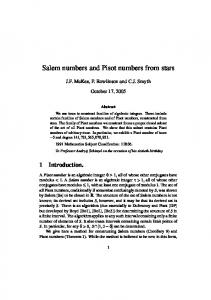
FIG. 1. – Horizontal velocity vectors at two levels separated by a distance δz, with the change in horizontal velocity given by (δu, δv). The sketches illustrate two extreme cases in which most of the shear is due to changes in velocity: (a) magnitude and (b) direction.

agating at different horizontal angles with respect to the mean flow. They found the fastest growing modes to be associated with local minima of the gradient Richardson number, consistent with observations of internal waves. Miller and Evans (1985), using data from ocean eddies initially generated as Gulf Stream rings, have shown that in most of the observations Ss is very similar to S. This indicates that usually the flow is locally almost parallel. However, they also showed that the relatively small proportion of cases in which shear is associated with changes in velocity direction accounts for almost as much shear as the cases in which shear is associated with changes in magnitude. Figure 1 illustrates the velocity vectors at two different depth levels (separated by a vertical distance δz) for rather different situations. In Figure 1a shear would be basically caused by changes in the magnitude of the current in the mean flow direction, so Equation (5) would closely apply. This case corresponds to shear instability in the direction of the mean alongstream flow, related to the background geostrophic flow as well as to ageostrophic contributions in the alongstream direction. In Figure 1b, on the other hand, shear is fundamentally caused by changes in the direction of the flow at both levels, so Equation (3) would be much more appropriate. One particular case leading to this situation could be a localised package of internal waves crossing a relatively weak mean alongstream flow. To calculate the geostrophic gradient Richardson number, Rig, we use the geostrophic velocity vg normal to a hydrographic section: ∂ρ −g ∂z Rig = 2 (6) ⎛ ∂v ⎞ , ρ⎜ g ⎟ ⎝ ∂z ⎠ where the vertical gradient ∂vg/∂z is calculated using the horizontal density gradients along a hydrographic section, by means of the thermal wind equation

∂vg

g ∂ρ . =− ∂z ρ f ∂x This leads to the following expression ∂ρ −ρ f 2 ∂z Rig = 2 ⎛ ∂ρ ⎞ . g⎜ ⎟ ⎝ ∂x ⎠

(7)

(6’)

The definition for the buoyancy frequency is the same as above, but we now define the geostrophic shear as Sg =

∂vg

∂z which allows us to write

=

Rig =

g ∂ρ , ρ f ∂x

N2 Sg

2

.

(8)

(6’’)

A comparison of Ss2 with Sg2 (equivalent to comparing Ris with Rig) should be informative on the role of ageostrophic along-stream motions leading to subcritical situations. At low vertical scales differences may arise because of the contribution of internal waves. At large vertical scales, we expect that the mean velocity of intense streams will approximately be in geostrophic balance, so when the hydrographic section is normal to the mean flow then these two Richardson numbers could give similar values. Deviations, however, may still arise because of frontogenetic processes in which the flow does not have enough time to reach geostrophy, something quite common in atmospheric jet streams with localised wind maxima (jet streaks). We expect that something similar may happen in intense largescale streams such as the Gulf Stream. Historical perspective and critical value The study of instabilities in stratified fluids started with the stability analysis of superposed fluids, i.e. fluids of different densities with an interface of


sm68n4459

7/12/04

10:19

Página 464

zero thickness (Helmholtz, 1868; Thomson (Lord Kelvin), 1910; see Lamb, 1932, and Chandrasekhar, 1961). The unstable perturbations at these interfaces have been named Kelvin-Helmholtz instabilities, or class C disturbances according to Benjamin’s (1963) classification. Other early authors also examined the mathematical problem of several layers of fluid and non-zero interface thickness (Taylor, 1931a; Goldstein, 1931), but detailed experimental confirmation of many of these results came much later (e.g. Thorpe, 1971, 1973; Scotti and Corcos, 1972). The name of Kelvin-Helmholtz instabilities, or billows, is now also commonly used to refer to the unstable perturbations that develop within a stratified shear flow. The first analysis of these perturbations was done by Geoffrey I. Taylor in his essay for the 1915 Adams Prize award. He examined the particular case of uniformly stratified and sheared flow (both N and S constants) and proved that when the gradient Richardson number is above 0.25 the flow would be stable (these results, however, were only published much later, Taylor, 1931a). Taylor considered the case of parallel flow so his definition for the gradient Richardson number corresponds to Ris (Equation 4). Later on, Lewis F. Richardson considered an energy balance equation to prove that the energy of turbulent fluctuations will increase when Ri (Equation 1) is less than one. Also using energy arguments, first Prandtl (1929) obtained that the critical number was 0.5 and later Taylor’s (1931b) results agreed with Richardson’s critical value of one. Much later, several authors followed the energy feasibility line to obtain a critical value of 0.25 (Chandrasekhar, 1961; Ludlam, 1967; Hines, 1971), but Miles (1986) amended these results to confirm a critical number of one. After Taylor’s (1931a) work, the analysis of the behaviour of small disturbances in stratified flows was undertaken by Synge (1933), Long (1955), and Drazin (1958). It was, however, Miles (1961) who first proved that the gradient Richardson number in parallel flow (Equation 4) had a critical value of 0.25. In his proof John Miles assumed that the velocity was monotonic and that the velocity and density fields had no discontinuities, but these restrictions were rapidly removed by Howard (1961). As Miles (1986) points out, the energetic requirements for particle exchange consider finite displacements while the condition for the growth of perturbations deals with infinitesimally small displacements. An additional difference is that the energy 464 P. VAN GASTEL and J.L. PELEGRÍ

approach is not restricted to parallel flow, and this is reflected in the definition used for the actual Richardson number (Equation 1). Abarbanel et al. (1984, 1986) have shown that the condition for nonlinear (Liapunov) stability of 3D stratified shear flow, which should now take into account finite displacements, leads to a critical Ri value of one, precisely the same condition that arises from energy considerations. DATA SET Hydrographic and velocity data For our analysis we used three different data sets for a very intense ocean current, the Gulf Stream (Fig. 2). Only one of these data sets has actual velocity measurements although its vertical resolution is only 25 m. The other two data sets have much better vertical resolution (1 and 10 m) so they allow us to examine the density structure at those scales. These data sets, however, lack actual velocity data which has to be inferred using the geostrophic approximation. Cape Hatteras Between September 1980 and May 1983 a series of 20 bimonthly temperature and velocity sections across the Gulf Stream were obtained near 73˚W (Halkin and Rossby, 1985). Each section contained between four and ten stations down to a depth of 2000 m, the spacing between stations being 25 km. Temperature observations were made with expandable bathythermographs (XBTs), providing data every 2 m. There is no data available for salinity but this was estimated from the temperature values through Armi and Bray’s (1983) algorithm in order to obtain the density field. Horizontal velocities were obtained every 25 m with a freefalling profiler named Pegasus, which is tracked through transponders located on the ocean floor (Spain et al., 1981). Here we have analysed this whole data set in a stream coordinate system, i.e. after each transect has been rotated to become perpendicular to the instantaneous direction of the Gulf Stream (Halkin and Rossby, 1985), provided to us courtesy of Prof. Tom Rossby from the University of Rhode Island. An analysis of the errors in the dependent variables caused by the XBTs limited accuracy and the

sm68n4459

7/12/04

10:19

Página 465

FIG. 2. – Location of all three data-set transects over a grey-coloured sea-surface temperature satellite image (available from the National Oceanic and Atmospheric Administration web page) that shows the path of the Gulf Stream as a band of relatively warm (dark) surface waters: (1) 25 m interval Pegasus (2 m interval XBT) data off Cape Hatteras, (2) 10 m interval CTD data along the 36°N section , and (3) 1 m interval CTD data in the Blake Plateau.

lack of salinity measurement was provided by Rodríguez-Santana et al. (1999), and some of the accuracy limitations associated with the Pegasus instrument have been discussed by Halkin and Rossby (1985). These assumptions, especially the applicability of a standard T-S relation, may appear as a large source of error and deserve special attention. Using an error propagation analysis (e.g. RodríguezSantana et al., 1999) we have the following expressions for the maximum relative errors: δN2/N2 = δz/∆z + δρ/∆ρ, δS2/S2 = δz/∆z + δu/∆u, and δRi/Ri = δN2/N2 + δS2/S2 = 2δz/∆z + δρ/∆ρ + δu/∆u, where δz, δu, and δρ represent the errors involved in measuring changes in the variables (at x, y constant): ∆z, ∆u = ∂u/∂z ∆z, and ∆ρ = ∂ρ/∂z ∆z. The depth change is ∆z = 25 m and estimates for the changes in velocity and density (using mean velocity and density profiles) are ∆u = 0.05 m s-1 and ∆ρ = 0.03 kg m-3. The maximum depth measurement error is estimated as that given by the pressure transponder

nominal accuracy (0.5%), δz = 0.005 ∆z. The velocity error is obtained from the accuracy of the Pegasus instruments, namely δu = 0.01 m s-1, giving δu ≅ 0.2 ∆u. A density measurement error could be estimated from the XBT accuracy (0.01ºC) as δρ = α ρ δT ≅ 0.002 kg m-3, where α ≅ 2 × 10-4 ºC-1 is the thermal expansion coefficient. A greater density error could possibly occur at small scales because of the T-S relationship assumption. Rodríguez-Santana et al. (1998) have shown that this relationship leads to a mean density error that decreases with increased vertical smoothing, from 0.010 kg m-3 over 5 m to 0.007 kg m-3 over 10 m. We have estimated that further smoothing of this data set to ∆z = 25 m gives δρ = 0.003 kg m-3, which is of the same order as our previous estimate. Hence, we may add both sources of error to give δρ ≅ 0.17 ∆ρ. Using these values we may estimate the maximum relative errors for both N2 and S2 to be about 0.2, while for Ri they may double. These relative errors are considerably large and


sm68n4459

7/12/04

10:19

Página 466

could indeed modify some of the details of our results, but we believe that the main spatial patterns (particularly when plotting logarithms) remain and the main conclusions will still hold. This is particularly true if we consider that these maximum relative errors are certainly overestimates of the actual relative errors, as shown by Rodriguez-Santana et al. (1998) through a Montecarlo simulation. 36°N section In September 1993 a conductivity-temperaturedepth (CTD) hydrographic section was made along 36°N on board the R/V Multanovsky. The chief scientist was Dr. Valdimir Tereschenkov and the data are available from the WOCE database (http://whpo.ucsd.edu). The whole transect comprised a total of 133 sampling sites but here we have only considered the 28 westernmost stations which cover the Gulf Stream region. The distance between each pair of stations varies from 10 to 15 km, the total transect distance being 400 km. Observations of pressure, salinity, and temperature are available every 10 db down to the sea bottom, in this area deeper than 2000 m except over the narrow continental slope.

ing interval, a consistent procedure as discussed by Miller and Evans (1985). The filter we chose is a running average filter given by 1 (n−1)/ 2 (9) ∑ x (i − j ) , n j =−(n−1)/ 2 where x(i) and y(i) are the input and output functions at a location given by z = iδz, and n is an odd integer that defines the smoothing interval nδz, the original sampling interval being δz. The transfer function of this filter is given by (e.g. Koopmans, 1974) y(i) =

sin(mn / 2 ) , (10) n sin(m / 2 ) with the non-dimensional vertical wavenumber m = 2π/l defined in terms of the non-dimensional vertical wavelength l = λ/δz, where λ is the dimensional wavelength. The transfer function is positive (zero phase function) when |m| ≤ 2π/n, otherwise it alterB( m ) =

Blake Plateau In September 1980 seven conductivity-temperature-depth (CTD) hydrographic sections were run across Blake Plateau (Atkinson, 1983). For our analysis we selected a relatively small portion (about 80 km long) of the transect located at approximately 31°N, provided to us courtesy of Prof. Larry Atkinson from Old Dominion University. This consists of only five stations, with an irregular spacing interval, that completely cover the rather narrow Gulf Stream in this area. Observations of pressure, salinity, and temperature are available every 1 db down to the sea bottom, in this area located somewhere between 300 and 550 m. Smoothing procedure To calculate the smoothed buoyancy frequency and shear values we followed what we believe is the simplest possible procedure. This consists in first smoothing the density and velocity fields by means of a symmetric average linear filter and then calculating the gradients as differences in density and velocity over vertical distances equal to the smooth466 P. VAN GASTEL and J.L. PELEGRÍ

FIG. 3. – (a) Shape of the transfer function of the running filter, and (b) its squared (power) value, for two different smoothing intervals.

sm68n4459

7/12/04

10:19

Página 467

nates between negative and positive values. The values of the function are rather small over the wavenumber where the transfer function is negative, which means that relatively little power is transmitted by the filter in this range. Figure 3a shows the shape of the transfer function for several smoothing intervals and Figure 3b shows its squared (power) value, the latter illustrating the good behaviour of the symmetric running filter with most of the energy retained for wavelengths l > n.

log Sg2 versus log N2 for different degrees of smoothing, as obtained from the Blake Plateau data. The increase in smoothing clearly results in the suppression of both highly stratified and well mixed regions (towards the background stratification) while the shear values remain essentially unaltered. The dashed line illustrates the Rig = 1 critical condition

RESULTS Throughout this section we use the above definitions to calculate the logarithms of the squared buoyancy frequency, the squared vertical shear, and the gradient Richardson number. Logarithms have two major advantages for our study. One advantage is that their distributions are well represented by a normal curve, which allows us to characterise a region with mean (or median) and standard deviation values. A second advantage is that their contouring permits a rather neat view of a large range of values, which is impossible with the actual number distributions. The logarithms of the squared buoyancy frequency and the squared vertical shear are always negative, the latter usually with a greater absolute value. The Richardson number, on the other hand, is computed as the difference between the two quantities, e.g. log Ri ≡ log N2 – log S2, and turns out to be a positive quantity except in subcritical regions. Recall that low (high) absolute log N2 values imply strong (weak) stratification, and low (high) absolute log S2 values imply strong (weak) shear. Hence, subcritical conditions take place when shear is strong and/or stratification is weak. As a reference, note that subcritical, critical and supercritical Ri values of 0.25, 1 and 10 correspond to log Ri values of -0.6, 0 and 1 respectively. We will see that subcritical conditions (log Ri < 0) do take place but in a very limited number of situations; the data, however, should also be able to indicate those conditions and regions that are prone to mixing and what happens with them after smoothing of the density and velocity fields. Geostrophic gradient Richardson number Let us first show some results obtained solely from the CTD data, with the help of the geostrophic approximation. Figure 4 shows a scatter diagram of

FIG. 4. – Scatter diagram of log Sg2 as a function of log N2 for the Blake Plateau data with (a) no smoothing, (b) 7 m smoothing, and (c) 21 m smoothing. The dashed line illustrates the Rig = 1 condition (log N2 = log Sg2).


sm68n4459

7/12/04

10:19

Página 468

FIG. 5. – Distribution of log Rig from the Blake Plateau data: (a) no smoothing, (b) 3 m smoothing, (c) 7 m smoothing, (d) 11 m smoothing, (e) 21 m smoothing, and (f) 51 m smoothing. Panels (a) and (b) show the 0.25, 0.5, and 1 contours, while the other panels have the 1 and 1.5 contours lines.

(log N2 = log Sg2), which is barely met by some original data points (where both shear and stratification are very weak) but disappears with smoothing as the low log N2 (well-mixed regions) vanish, while the log Sg2 values remain essentially unaltered. A close inspection of the actual log N2 distribution (not shown) indicates that most stratified regions are located at the base of the seasonal mixed layer and 468 P. VAN GASTEL and J.L. PELEGRÍ

within the top 200 m of the Gulf Stream, while wellmixed regions are spread over the whole section. As we smooth the data most patches of low and high stratification disappear, although a 51 m smoothing is necessary to eliminate some persistent well-stratified patches located either near the base of the seasonal thermocline (some 50 m deep) or at depths of some 100 m within the Gulf Stream.

sm68n4459

7/12/04

10:19

Página 469

Figure 5 presents the distribution of the minimum log Rig values for different smoothing intervals, again from the Blake Plateau data. This distribution reflects the controlling roles of stratification all the way up to a smoothing of 21 m, with the minimum values clearly associated with well-mixed regions. The distribution of log Sg2 (not shown) consists of a band of moderately large values (|log Sg2| ≈ 5.5) at the location of the Gulf Stream, below the surface mixed layer. When one of the well-mixed regions is associated with a moderately high velocity shear then we get log Rig values below one. Values below zero (subcritical regions) only appear when one is using the original 1 db data, usually coinciding with density inversions in the water column. Only for smoothing over distances above 11 m does shear become the dominant factor controlling the log Rig distribution. Figure 6 displays similar results for log Rig but now obtained from the 36°N data set (note the change in the cross-stream scale as compared with

Figure 5). The low Richardson values are partly controlled by stratification only at the highest vertical resolution of these data (10 m), this case being characterised by a more patchy structure. As smoothing increases, the patchiness is rapidly reduced and the values increase, so when smoothing reaches 110 m we have a rather broad band of moderately low values that follows the shape of the Gulf Stream. The less stable regions (log Ri below 1) again follow the shape of the Gulf Stream, except near the surface mixed layer where shear is small. Figures 7 to 10 present the effect of smoothing on the distribution of log N2, log Sg2, and log Rig, as obtained now from the Pegasus data set off Cape Hatteras (again note the change in the cross-stream scale as compared with the previous figures). Since the velocity data is available at 25 m intervals our first step was to smooth the original density data (available every 2 m) over this longer vertical interval to obtain what we used as the 25 m density data. The distribution of the maximum buoyancy frequen-

FIG. 6. – Distribution of log Rig from the 36°N transect data with (a) no smoothing, (b) 30 m smoothing, (c) 70 m smoothing, and (d) 110 m smoothing. All panels show the 0.25, 0.5, and 1 contour lines.


sm68n4459

7/12/04

10:19

Página 470

FIG. 7. – Distribution of log N2 from the Cape Hatteras data showing the strongly stratified regions with (a) 25 m smoothing, (b) 75 m smoothing, (c) 175 m smoothing, and (d) 275 m smoothing. All panels show the -4.1, -4.0, -3.9, and -3.8 contour lines.

FIG. 8. – Distribution of log Sg2 from the Cape Hatteras data with (a) 25 m smoothing, (b) 75 m smoothing, (c) 175 m smoothing, and (d) 275 m smoothing. All panels show the -5.6, -5.5, -5.4, and -5.3 contour lines.


sm68n4459

7/12/04

10:19

Página 471

cies (Figure 7) changes very little for smoothing intervals greater than 25 m, with the most stratified regions being located immediately below the seasonal thermocline and in the top few hundred metres within the Gulf Stream. High absolute values (not shown) appear in the shallow surface mixed layer or towards the less stratified deep layers. The distribution shows very little structure within the Gulf Stream core for these large vertical smoothing intervals, in accordance with our previous results for smoothing intervals of 10 m or more. Figure 8 illustrates the distribution of the lowest log Sg2 absolute values (maximum shear regions), which are associated with both the base of the seasonal thermocline and the Gulf Stream itself. Increased smoothing gets rid of the high shear at the base of the thermocline, but the high shear Gulf Stream regions remain essentially unchanged. Figure 9 presents the distribution of the lowest log Rig values (less stable regions). At these relatively large vertical scales (> 25 m) the Richardson values mainly respond to the structure of the shear, even at the base of the seasonal mixed layer. The shape of the region with relatively small log Rig values is tilted following the shape of the Gulf Stream maximum

velocity axis, again aside from the surface mixed layer. For the 25 m data the values are roughly between 0.8 and 1.5, i.e. actual Ri values approximately between 6 and 30, and increase little with smoothing. Figure 10 presents the corresponding scatter diagrams of log Sg2 versus log N2. The diagram suffers very minor modifications as smoothing increases, being always far away from the critical regions illustrated by the dashed line in this figure. Synoptic and actual gradient Richardson numbers Let us now turn to the estimates for shear and gradient Richardson number obtained with the actual Pegasus velocity measurements off Cape Hatteras. As mentioned above the data is analysed in a coordinate system rotated to be aligned with the instantaneous Gulf Stream direction, as defined by the maximum depth-integrated transport (Halkin and Rossby, 1985). This selection ensures that crossstream motions are not simply due to any misalignment between the direction of the stream and the orientation of the geographic system (defined by the location of the bottom transducers).

FIG. 9. – Distribution of log Rig from the Cape Hatteras data with (a) 25 m smoothing, (b) 75 m smoothing, (c) 175 m smoothing, and (d) 275 m smoothing. All panels show the 1.0, 1.25, and 1.5 contour lines.


sm68n4459

7/12/04

10:19

Página 472

FIG. 10. – Scatter diagram of log Sg2 as a function of log N2 for the Cape Hatteras data with (a) 25 m smoothing, (b) 75 m smoothing, (c) 175 m smoothing, and (d) 275 m smoothing. The dashed line illustrates the Rig = 1 condition (log N2 = log Sg2).

FIG. 11. – (a) Measured and (b) geostrophic velocity fields off Cape Hatteras for March 1982. Units are in m s-1.

Halkin and Rossby (1985) provided a very careful description of the along-stream and cross-stream velocity components for the March 1982 realisation (their Figure 6) and the mean ensemble (their Figures 10 and 11). Figure 11a illustrates the along-stream velocity component as obtained from the actual velocity data, which essentially reproduces Figure 6b 472 P. VAN GASTEL and J.L. PELEGRÍ

in Halkin and Rossby (1985). This may be compared with the along-stream geostrophic velocity field, as determined from the temperature data and with the help of Armi and Bray’s (1983) algorithm to obtain the salinity values, after its projection onto the stream coordinate system (Fig. 11b). The velocity fields are indeed quite similar, in concordance with

sm68n4459

7/12/04

10:19

Página 473

FIG. 12. – Distribution of log Ss2 from the Cape Hatteras data with (a) 25 m smoothing, (b) 75 m smoothing, (c) 175 m smoothing, and (d) 275 m smoothing. Distribution of log S2 from the Cape Hatteras data with (e) 25 m smoothing, and (f) 75 m smoothing. All panels show the -5.4, -5.2, -5.0 and -4.8 contour lines.

the results of Johns et al. (1989). The actual velocity field, however, is not only slightly more intense but exhibits more small scale variability. Figures 12a-d present the log Ss2 distributions for different smoothing intervals. The high shear regions are located within the Gulf Stream axis or along its cyclonic side (to the left of the stream core when facing downstream), with maximum values

taking place at the base of the seasonal thermocline. As smoothing increases the high shear in the surface layers disappears but the maximum shear regions within the upper thermocline layers of the Gulf Stream experience few changes. Figures 12e,f illustrate the log S2 for the original (25 m) data and low smoothing (75 m) interval. They show that the actual shear is usually slightly higher than the synoptic


sm68n4459

7/12/04

10:19

Página 474

FIG. 13. – Distribution of log Ris from the Cape Hatteras data with (a) 25 m smoothing, (b) 75 m smoothing, (c) 175 m smoothing, and (d) 275 m smoothing. Distribution of log Ri from the Cape Hatteras data with (e) 25 m smoothing, and (f) 75 m smoothing. All panels show the 0.25, 0.5, 0.75 and 1.0 contour lines.

shear in the cyclonic side of the current and, most noticeably, it also presents high values within the surface layers of the anticyclonic side of the stream. The log S2 distributions for greater smoothing intervals differ very little from the log Ss2 ones (Figs. 12c,d) and are not shown. Figure 13 displays the corresponding log Ris (Figs. 13a-d) and log Ri (Figs. 13e,f) distributions, calculated from the fields shown in Figures 7 and 474 P. VAN GASTEL and J.L. PELEGRÍ

12, and according to the definitions (1’) and (4’). For the 25 and 75 m smoothing intervals the high shear in the surface anticyclonic layers has little impact on the Richardson values, which is indicative that these are also well stratified layers. Perhaps surprisingly, the 25 m distributions display many subcritical regions (negative log Ri) scattered away from the stream itself. These respond to moderate shear and little stratification in relatively deep

sm68n4459

7/12/04

10:19

Página 475

FIG. 14. – Scatter diagram of log Ss2 as a function of log N2 for the Cape Hatteras data with (a) 25 m smoothing, (b) 75 m smoothing, (c) 175 m smoothing, and (d) 275 m smoothing. The dashed line illustrates the Ris = 1 condition (log N2 = log Ss2).

regions, in contrast to the high shear regions within the Gulf Stream. For smoothing intervals of 75 m and above the distributions of both log Ri (not shown) and log Ris are very similar, with relatively low Richardson values only within the upper-thermocline high-shear layers of the Gulf Stream. These would correspond to those statically stable but dynamically unstable regions discussed by Pelegrí and Csanady (1994) and Pelegrí and Sangrà (1998), where the diapycnal shear (the rate of change of velocity with density) is the critical quantity. Figure 14 presents the scatter diagram of log Ss2 versus log N2 for different smoothing intervals (the corresponding scatter diagrams of log S2 versus log N2 are not shown because they are very similar). A comparison with the corresponding geostrophic results (Fig. 10) shows that for the 25 m data interval the maximum actual shear is about twice the maximum geostrophic shear, with the difference diminishing as the vertical smoothing interval increases. The minimum actual shear values, on the other hand, are about two orders of magnitude greater than the minimum geostrophic shear values. The results indicate that at these scales the flow in

some regions approaches but never reaches the subcritical condition. DISCUSSION Effect of smoothing on gradient Richardson values Table 1 and Figure 15 correspond to the Blake Plateau data. Table 1 presents the median values for the Gaussian curves adjusted to log N2, log S2, and log Rig for the original and smoothed data. The original, 1-m data have a number of inversions (about 10% of the data) which have been removed from the calculations. The table also displays the standard deviation and regression coefficients of the highly smoothed log Rig data with respect to the 3-m smoothed log Rig data. Figure 15 shows the Gaussian curves fitted to the log Rig distribution for 7 m, 51 m, and 201 m smoothing intervals. These results clearly show that the overall distributions are little affected by smoothing, though we are dealing with a relatively small section through the Gulf Stream.


sm68n4459

7/12/04

10:19

Página 476

TABLE 1. – Summary of results obtained with the Blake Plateau data. Median and standard deviation values from the original and smoothed (3, 7, 11, 21 and 51 m) log N2, log Sg2, and log Rig data. Also shown are the regression coefficients of the greatly smoothed log Rig data with respect to the 3 m smoothed log Rig data.

No smoothing 3 m smoothing 7 m smoothing 11 m smoothing 21 m smoothing 51 m smoothing

Median (s.d.) log N2

Median (s.d) log Sg2

-4.05 -4.11 -4.14 -4.14 -4.14 -4.14

-6.86 -6.86 -6.89 -6.90 -6.90 -6.92

(3.77) (3.93) (3.99) (4.02) (4.05) (4.09)

FIG. 15. – Gaussian curves adjusted to log Rig, obtained with several smoothing intervals of the Blake Plateau data (7 m, dashed line; 51 m, solid line; 201 m, dotted line).

This indicates that most fine density structure occurs at vertical scales below 7 m, and that horizontal temperature gradients (geostrophic vertical shear) change little with depth. Nevertheless, it is important to realise that if we were to choose a very specific region, such as the one with relatively small Rig values in Figure 5, this result would not necessarily hold any longer. Table 2 summarises the results for log Rig but now obtained from the 36°N data set. The median Richardson values in the 36°N section are considerTABLE 2. – Summary of results with the 36°N transect data. Median and standard deviation values for log Rig from the original and smoothed (30, 70, 110 and 210 m) data. Also shown are the regression coefficients of the smoothed values with respect to the unsmoothed data. Median (s.d) log Rig No smoothing 30 m smoothing 70 m smoothing 110 m smoothing 210 m smoothing

3.63 3.72 3.74 3.74 3.78

(1.39) (1.53) (1.54) (1.53) (1.54)


Reg. Coeff.

1.00 1.01 1.02 1.02 1.02

(5.54) (5.54) (5.54) (5.55) (5.56) (5.79)

Median (s.d) log Rig 2.93 2.82 2.82 2.84 2.85 2.89

(1.22) (1.25) (1.17) (1.15) (1.17) (1.29)

Reg. Coeff. 1.00 0.98 0.98 0.99 1.02

ably larger than those obtained from the Blake Plateau section, and the standard deviations are also significantly larger. This shows that the absolute values depend very much on the extent and location of the section under consideration. The higher median values for the 36°N section, for example, should be expected simply because the 36°N section encompasses many interior gyre stations (i.e. a smaller fraction of the stations are within the potentially dynamically unstable Gulf Stream waters). Let us finally turn to the Cape Hatteras data in which we have available actual velocity values. Figure 16 presents the data histograms of log Ris and log Rig for the Cape Hatteras data with different degrees of smoothing. On these histograms we have drawn the corresponding Gaussian curves which adjust rather well to the end values in the distribution, which would not have happened if we had not used the logarithm of the variables. In concordance with our previous results, the distribution of log Rig is very little affected by smoothing. The log Ris histogram, however, is clearly affected by smoothing, particularly when going from 25 to 175 m, which is indicative of the existence of ageostrophic motions on these vertical scales. At vertical scales over 75 m these motions are in the alongstream direction, but below this scale a significant contribution comes from cross-stream motions (Fig. 13). Figure 17 and Table 3 summarise the main results for the Cape Hatteras data. Figure 17 clearly shows the difference between the Gaussian curves adjusted to the log Ris and log Rig data, illustrating the small (high) effect of smoothing on the geostrophic (synoptic) values. Table 3 includes the median and standard deviation values for log N2, log Sg2 (log Ss2 and log S2), and log Rig (log Ris and log Ri), for different smoothing intervals. The median and standard deviation values for log Rig are very similar to the 36°N values, as could be expected both because of the geographical closeness between

sm68n4459

7/12/04

10:19

Página 477

FIG. 16. – Histograms of log Ris from the Cape Hatteras data with (a) 25 m smoothing, (b) 75 m smoothing, (c) 175 m smoothing, and (d) 275 m smoothing. Histograms of log Rig from the Cape Hatteras data with (e) 25 m smoothing, (f) 75 m smoothing, (g) 175 m smoothing, and (h) 275 m smoothing.


sm68n4459

7/12/04

10:19

Página 478

FIG. 17. – Gaussian curves adjusted to log Ris (solid line: unsmoothed; dashed line: 275 m smoothed) and log Rig (dotted line: unsmoothed; dotted-dashed line: 275 m smoothed), obtained with the Cape Hatteras data.

the two sections and because of the similar fraction of Gulf Stream stations (though the 36°N transect is longer than the Cape Hatteras one). The median Ris values are between one and two orders of magnitude lower than the median Rig, the difference decreasing with smoothing because of the noticeable increase in Ris. The standard deviation is little affected by smoothing, being about 0.5 for log Ris and 1.2 for log Ris. The regression coefficients of the greatly smoothed data with respect to the 25 m smoothed data are also included in Table 3 for both log Ris and log Rig. These coefficients are always very close to one for log Rig, but for log Ris they increase considerably with smoothing. Table 3 also illustrates how the Gaussian distributions behave when the amount of available data is decimated through a block average (in opposition to a running average). This procedure would approximately resemble the case of instruments measuring over vertical bins, such as Doppler profilers. In this case the 75, 175 and 275 m decimated data would

have only one out of every three, seven, and eleven original data points respectively. The geostrophic values are not substantially modified, in contrast with the median synoptic values which increase with the decimating interval. Table 3 shows that the median values for log N2 are indeed not affected by smoothing, their values being those of the background stratification. Nor can vertical smoothing change the large-scale slope of the isopycnals, which determines the geostrophic flow and the geostrophic shear log Sg2. Fine structure (such as that induced by localised mixing and/or the passage of internal waves) may change the local slope of the isopycnals but this change would occur over distances much shorter than the internal Rossby radius of deformation, so any associated change in the flow would not be in geostrophic balance. The (smoothed and unsmoothed) geostrophic velocities are solely calculated from the density values, so we could have anticipated the similar behaviour in the median values for the squared buoyancy and geostrophic gradient Richardson number. The median values of the synoptic shear log Ss2, on the other hand, clearly decrease with smoothing at a similar rate as log Ris does. The actual median shear, log S2, and Richardson, log Ri, values display a similar pattern as the synoptic ones, but their absolute values are about 0.3-0.5 units lower. Finally, in Figure 18 we present several scatter diagrams that illustrate the effect of smoothing on both log Ris and log Rig, with the smoothed data plotted as a function of the unsmoothed data. Smoothing has a very great effect on the individual Ris values, changing them typically by two orders of magnitude and as much as four orders of magnitude. On the other hand, the individual Rig values usually retain the same original order of magnitude after smoothing, with the maximum increase being two orders of magnitude when smoothing is performed with a 275 m vertical interval.

TABLE 3. – Summary of results obtained with the Cape Hatteras data. Median and standard deviation values for the log Ris, log Rig, log Ri, log N2, log Sg2, log Ss2, and log S2 original and smoothed (75, 175, 275 and 525 m) data. Also shown are the median and standard deviation values for the log Ris and log Rig decimated (75, 175 and 275 m) data, and the regression coefficients of the highly smoothed and decimated log Rig and log Ris values with respect to the 25 m log Rig and log Ris data respectively.

No 75 m smo. 175 m smo. 275 m smo. 525 m smo. 75 m dec. 175 m dec. 275 m dec.

Median (s.d) Reg. Median (s.d) Reg. log Ris Coeff. log Rig Coeff.

Median (s.d) Median (s.d) Median (s.d) Median (s.d) Median (s.d) log Ri log N2 log Sg2 log Ss2 log S2

1.33 1.63 2.02 2.20 2.40 1.88 2.02 2.37

0.89 1.25 1.58 1.76 2.03

(0.50) (0.47) (0.52) (0.54) (0.61) (0.54) (0.49) (0.57)

1.000 1.165 1.331 1.412 1.513 1.263 1.361 1.539

3.52 3.55 3.55 3.44 3.47 3.95 3.23 3.09


(1.19) (1.16) (1.18) (1.16) (1.15) (1.25) (1.21) (1.16)

1.000 0.990 0.994 0.995 0.997 1.069 0.816 0.860

(1.11) (1.46) (2.01) (1.91) (2.23)

-4.33 -4.33 -4.33 -4.33 -4.35

(4.75) (4.72) (4.79) (4.84) (4.84)

-7.88 -7.87 -7.84 -7.78 -7.82

(6.10) (6.12) (6.15) (6.18) (6.32)

-6.71 -7.03 -7.33 -7.42 -7.63

(5.78) (5.90) (6.02) (6.01) (6.05)

-6.21 -6.57 -6.99 -7.08 -7.35

(5.53) (5.79) (5.99) (5.99) (6.04)

sm68n4459

7/12/04

10:19

Página 479

FIG. 18. – Scatter diagrams with the Cape Hatteras data. Smoothed log Ris values (a: 75 m, b: 175 m, and c: 275 m) plotted as a function of 25 m log Ris values. Smoothed log Rig values (d: 75 m, e: 175 m, and f: 275 m) plotted as a function of 25 m log Rig values.

Shear mixing from high to low vertical wavenumbers The vertical resolution of our Gulf Stream data is only suitable for examining the effect of geostrophic shear at fine structure scales (1 to 3 m) and actual shear at relatively large scales (25 m or more). Let

us first briefly consider the potential role of geostrophic shear at fine structure scales, and how this may be enhanced through internal waves. One remarkable feature in our 1-m interval data (Fig. 5a) is the existence of numerous density inversions within the Gulf Stream stations, reaching close to 10% of the observations. After removing all these


sm68n4459

7/12/04

10:19

Página 480

inversions we still have several locations (at 1 and 3 m vertical resolution) where the geostrophic gradient Richardson values are near critical. Further vertical smoothing removes these well-mixed regions and N2 increases, while the geostrophic shear (S2) remains essentially unchanged. This suggests that the small-scale, well-mixed regions have their origin in high-shear at small scales, such as that caused by internal waves. It is probable that the relatively intense background shear in the Gulf Stream sets up the right near-critical conditions, but actual subcritical conditions appear to occur through the reinforcement of this mean shear by internal waves (Garrett and Munk, 1972b; Turner, 1973; Munk, 1981; Thorpe, 1999). At large vertical scales, on the other hand, the localised effect of internal waves can only play a minor role. At these scales we may expect that critical conditions will be attained whenever the Gulf Stream becomes sufficiently intensified, possibly related to some meander phases. The variability in the Stream’s maximum velocity and structure (Rossby and Gottlieb, 1998; Rossby and Zhang, 2001) appears to be largely related to changes in its structure during different meander phases (Newton, 1978; Bane et al., 1981; Rodríguez-Santana et al., 1999). During these meanders the mean stratification (∂z/∂ρ) remains essentially unchanged, while the slope of the isopycnals is largely modified— quite the opposite of what happens at small vertical scales. Following Pelegrí and Csanady (1994), we may take this fact into consideration by writing the geostrophic gradient Richardson number (Equation 6) in isopycnic coordinates: ∂z −g ∂ρ Rig = 2 , (6’’’) ⎛ ∂vg ⎞ ρ⎜ ⎟ ⎝ ∂ρ ⎠ and using the thermal wind equation in isopycnic coordinates ∂vg

g ∂z , ρ f ∂x

(7’)

∂z ∂ρ , Rig = 2 ⎛ ∂z ⎞ g⎜ ⎟ ⎝ ∂x ⎠

(6’’’)

∂ρ

=

to obtain f 2ρ


Observations on the northern Blake Plateau (Bane et al., 1981; Rodríguez-Santana et al., 1999) have shown that the slope of the isopycnals (∂z/∂x) increases by a factor of four in a time period of only six days, as a response to the compression of the cross-stream horizontal coordinate. Under these conditions the gradient Richardson number would decrease by a factor of 16 and possibly lead to critical values. Once these conditions are attained, shear instabilities could rapidly develop, with temporal and vertical scales being a function of the background stratification, and lead to mixing and fine structure. CONCLUSIONS We have examined the distribution of the buoyancy frequency, vertical shear and gradient Richardson number for several sections across a very intense oceanic current. The different data sets have been smoothed using several vertical intervals. The smoothing allows us to examine the differences that may arise when the gradient Richardson number is estimated with different types of instruments. Most important, however, this smoothing procedure together with the use of different complementary definitions (actual, synoptic, and geostrophic) provides information on how shear mixing may be taking place at different vertical scales as a result of several mechanisms. The results show that the logarithms of the buoyancy frequency, vertical shear and gradient Richardson number may be fairly well approximated with Gaussian distributions. The actual mean and standard deviation values depend primarily on the dynamic characteristics of the section under consideration. For distributions obtained from Gulf Stream sections with similar dynamic regimes, these values also depend on the relative fraction of Gulf Stream stations. As this fraction decreases, for example, the median gradient Richardson number increases. Within one specific section smoothing has little effect on the distribution of the log N2, log Sg2, and log Rig. It does have a major effect on the median values of the distribution of the synoptic (log Ss2 and log Ris) and actual (log S2 and log Ri) values, which increase by a factor approximately proportional to the smoothing factor, but a relatively minor effect on the respective standard deviations. The results suggest that within the Gulf Stream frequent shear-induced mixing takes place at the

sm68n4459

7/12/04

10:19

Página 481

fine-structure scale, as the combined result of the mean geostrophic velocity field and ageostrophic motions. Geostrophic shear within the Gulf Stream is associated with near-critical conditions in 1-m interval data, but only in already well-mixed regions that rapidly disappear with vertical smoothing. For vertical scales of 5-10 m or above, the geostrophic shear is not enough to induce shear-mixing. At these short vertical scales, hence, intense geostrophic shear preconditions the occurrence of near-critical conditions although actual mixing may only take place through the action of small-scale ageostrophic processes, probably internal waves. Actual velocity measurements show that for vertical scales of 25 m or larger the ageostrophic motions within the Gulf Stream are still intense enough to produce the near-critical conditions locally. At these scales the cross-stream ageostrophic contributions are smaller than the corresponding along-stream contributions, though they are not negligible. We propose that actual subcritical conditions at these vertical scales take place because of the local acceleration of western boundary currents during frontogenetic phases of meanders. ACKNOWLEDGEMENTS The authors are grateful to Tom Rossby, University of Rhode Island, and Larry Atkinson, Old Dominion University for kindly providing data sets. We would also like to thank Bob Haney, Naval Postgraduate School, and Bill Smyth, Oregon State University, for a number of very useful comments. Part of this work was written while J.L.P. was at University of Wisconsin-Madison with a grant from the Ministerio de Educación, Cultura y Deportes, Spanish Government. This work has been partly funded by the European Union through the OASIS project (contract No. EVK3-CT-2002-00073-OASIS). REFERENCES Abarbanel, H.D.I., D.D. Holm, J.E. Mardsen, and R. Ratiu. – 1984. Richardson number criterion for the nonlinear stability of threedimensional stratified flow. Phys. Rev. Lett., 52: 2352-2355. Abarbanel, H.D.I., D.D. Holm, J.E. Mardsen, and R. Ratiu. – 1986. Nonlinear stability analysis of stratified fluid equilibria. Phil. Trans. R. Soc. Lond., 318: 349-409. Alford, M.H. and R. Pinkel. – 2000. Observations of overturning in the thermocline: The context of ocean mixing. J. Phys. Oceanogr., 30: 805-832. Armi, L. and N.A. Bray. – 1982. A standard analytic curve of potential temperature versus salinity for the western North Atlantic. J. Phys. Oceanogr., 12: 384-387.

Atkinson, L.P. – 1983. Distribution of Antarctic Intermediate Water over the Blake Plateau. J. Geophys. Res., 88: 4699-4704. Bane, J.M., Jr., D.A. Brooks and K.R. Lorenson. – 1981. Synoptic observations of the three-dimensional structure and propagation of Gulf Stream meanders along the Carolina continental margin. J. Geophys. Res., 86: 6411-6425. Benjamin, T.B. – 1963. The threefold classification of unstable disturbances in flexible surfaces bounding inviscid flows. J. Fluid Mech., 16: 436-459. Bruno M., J.J. Alonso, A. Cozar, J. Vidal, A. Ruiz-Cañavate, F. Echevarría and J. Ruiz. – 2002. The boiling-water phenomena at Camarinal Sill, the Strait of Gibraltar. Deep-Sea Res. II, 49: 4097-4113. Chandrasekhar, S. – 1961. Hydrodynamic and Hydromagnetic Stability. Oxford, 654 pp. Cisneros-Aguirre, J., J.L. Pelegrí and P. Sangrà. – 2001. Experiments on layer formation in stratified shear flow. Sci. Mar., 65(S1): 117-126. De Silva, I.P.D., H.J.S. Fernando, F. Eaton and D. Herbert. – 1996. Evolution of Kelvin-Helmholtz billows in nature and laboratory. Earth. Planet. Sci. Lett., 143: 217-231. Drazin, P.G. – 1958. The stability of a shear layer in an unbounded heterogeneous inviscid fluid. J. Fluid Mech., 4: 214-224. Evans, D.L. – 1982. Observations of small-scale shear and density structure in the ocean. Deep-Sea Res., 29: 581-595. Gargett, A.E., P.J. Hendricks, T.B. Sanford, T.R. Osborn and A.J. Williams III. – 1981. A composite spectrum of vertical shear in the upper ocean. J. Phys. Oceanogr., 11: 1258-1271. Gargett, A.E., T.R. Osborn and P.W. Nasmyth. – 1984. Local isotropy and the decay of turbulence in a stratified fluid. J. Fluid Mech., 144: 231-280. Garrett, C., and W. Munk. – 1972a. Space-time scales of internal waves. Geophys. Fluid Dyn, 3: 225-264. Garrett, C., and W. Munk. – 1972b. Oceanic mixing by breaking internal waves. Deep-Sea Res., 19: 823-832. Garrett, C., and W. Munk. – 1975. Space-time scales of internal waves: A progress report. J. Geophys. Res., 80: 291-297. Garrett, C., and W. Munk. – 1979. Internal waves in the ocean. Ann. Rev. Fluid Mech., 11: 339-369. Goldstein, S. – 1931. On the stability of superposed streams of fluids of different densities. Proc. R. Soc. London A, 132: 524-548. Gregg, M.C., E.A. D’Asaro, T.J. Shay and N. Larson. – 1986. Observations of persistent mixing and near-inertial internal waves. J. Phys. Oceanogr., 16: 856-885. Gregg, M.C., D.P. Winkel and T.B. Sanford. – 1993a. Varieties of fully resolved spectra of vertical shear. J. Phys. Oceanogr., 23: 124-141. Gregg, M.C., H.E. Seim and D.B. Percival. – 1993b. Statistics of shear and turbulent dissipation profiles in random internal wave fields. J. Phys. Oceanogr., 23: 1777-1799. Halkin, D. and T. Rossby. – 1985. The structure and transport of the Gulf Stream at 73°W. J. Phys. Oceanogr. 15: 1439-1452. Hazel, P.G. – 1972. Numerical studies of the stability of inviscid parallel shear flows. J. Fluid Mech., 51: 39-62. Helmholtz, H. – 1868. Uber discontinuirliche Flüssigkeitsbewegungen. Berl. Monatsber. Dtsch. Akad. Wiss Berlin, 23: 215-228. Hines, C.O. – 1971. Generalizations of the Richardson criterion for the onset of atmospheric turbulence. Quart. J. R. Met. Soc., 97: 429-439. Howard, L.N. – 1961. Note on a paper of John W. Miles. J. Fluid Mech., 10: 509-512. Itsweire, E.C., J.R. Koseff, D.A. Briggs and J.H. Ferziger. – 1993. Turbulemce in stratified shear flows: Implications for interpreting shear-induced mixing in the ocean. J. Phys. Oceanogr., 23: 1508-1522. Johns, E., D.R. Watts and H.T. Rossby. – 1989. A test of geostrophy in the Gulf Stream, J. Geophys. Res., 94: 3211-3222. Koopmans, L.H. – 1974. The spectral analysis of time series. Academic Press, London, 366 pp. Kundu, P.K. and R.C. Beardsley. – 1991. Evidence of a critical Richardson number in moored measurements during the upwelling season off Northern California. J. Geophys. Res., 96: 4855-4868. Kunze, E., A.J. Williams, and M.G. Briscoe. – 1990. Observations of shear and vertical stability from a neutrally buoyant float. J. Geophys. Res., 95: 18127-18142. Lamb, H. – 1932. Hydrodynamics. Cambridge University Press, Cambridge, 738 pp.


sm68n4459

7/12/04

10:19

Página 482

Ledwell, J.R., E.T. Montgomery, K.L. Polzin, L.C. St. Lauren, R.W. Schmitt and J.M. Toole. – 2000. Evidence for enhanced mixing over rough topography in the abyssal ocean. Nature, 403: 179-182. Long, R.R. – 1955. Some aspects of the flow of stratified fluids. III. Continuous density gradients. Tellus, 7: 342-357. Ludlam, F.H. – 1967. Characteristics of billow clouds and their relation to clear-air turbulence. Quart. J. R. Met. Soc., 93: 419435. Marmorino, G.O., L.J. Rosenblum and C.L. Trump. – 1987. Finescale temperature variability: The influence of near-inertial waves. J. Geophys. Res., 92: 13049-13062. Miles, J.W. – 1961. On the stability of heterogenous shear flows. J. Fluid Mech., 10: 496-508. Miles, J.W. – 1986. Richardson’s criterion for the stability of stratified shear flow. Phys. Fluids, 29: 3470-3471. Miller, J.L. and D.L. Evans. – 1985. Density and velocity fine structure enhancement in oceanic eddies. J. Geophys. Res., 90: 4793-4806. Moin, P. and K. Mahesh. – 1998. Direct numerical simulation: A tool in turbulence research. Annu. Rev. Fluid Mech., 30: 539-578. Munk, W. – 1981. Internal waves and small-scale processes. In: B.A. Warren and C. Wunsch (eds.), Evolution of Physical Oceanography, pp. 264-291. MIT Press, Cambridge. Newton, C.W. – 1978. Fronts and wave disturbances in Gulf Stream and atmospheric jet stream. J. Geophys. Res., 83: 4697-4706. Pelegrí, J.L. – 1988. Tidal fronts in estuaries. Est. Coastal Shelf Sci., 27: 45-60. Pelegrí, J.L. and G.T. Csanady. – 1991. Nutrient transport and mixing in the Gulf Stream. J. Geophys. Res., 96: 2577-2583. Pelegrí, J.L. and G.T. Csanady. – 1994. Diapycnal mixing in western boundary currents. J. Geophys. Res., 99: 18275-18304. Pelegrí, J.L. and G.T. Richman. – 1993. On the role of shear mixing during transient coastal upwelling. Cont. Shelf Res., 12: 1363-1400. Pelegrí, J.L. and P. Sangrá. – 1998. A mechanism for layer formation in stratified geophysical flows. J. Geophys. Res., 103: 30679-30693. Pelegrí, J.L., A. Rodríguez-Santana, P. Sangrá and A. MarreroDíaz. – 1998. Modeling of shear-induced diapycnal mixing in frontal systems. Appl. Sci. Res., 59: 159-175. Pingree, R.D. and A.L. New. – 1989. Downward propagation of internal tidal energy into the Bay of Biscay. Deep-Sea Res. A, 36: 735-758. Polzin, K.L., J.M. Toole, J.R. Ledwell and R.W. Schmitt. – 1997. Spatial variability of turbulent mixing in the abyssal ocean. Science, 276: 93-96. Prandtl, L. – 1930. Einfluß stabilisierender Fräfte auf die Turbulenz. Vorträge aus dem Gebiete der Aerodynamik und verwandten Gebieten, pp. 1-7. Springer, Berlin. Richardson, L.F. – 1920. The supply of energy from and to atmospheric eddies. Proc. R. Soc. London A, 97: 354-373. Rodríguez-Santana, A., J.L. Pelegrí, P. Sangrà and A. MarreroDíaz. – 1999. Diapycnal mixing in Gulf Stream meanders, J. Geophys. Res., 104: 25891-25912. Rossby, T. and E. Gottlieb. – 1998. The Oleander project: monitor-


ing the variability of the Gulf Stream and adjacent waters between New Jersey and Bermuda. Bull. Amer. Meteor. Soc., 79: 5-18. Rossby, T and H.M. Zhang. – 2001. The near-surface velocity and potential vorticity structure of the Gulf Stream. J. Mar. Res., 59: 949-975. Scotti, R.S., and G.M. Corcos. – 1972. An experiment on the stability of small disturbances in a stratified shear layer. J. Fluid Mech., 52: 499-528. Simpson, J.H. – 1975. Observations of small scale vertical shear in the ocean. Deep-Sea Res., 22: 619-627. Smyth, W.D. and J.N. Moum. – 2000. Length scales of turbulence in stably stratified mixing layers. Phys. Fluids, 12: 1327-1342. Smyth, W.D., J.N. Moum and D.R. Caldwell. – 2001. The efficiency of mixing in turbulent patches: inferences from direct simulations and microstructure observations. J. Phys. Oceanogr., 31: 1969-1992. Spain, P.F., D.L. Dorson and H.T. Rossby. – 1981. PEGASUS, a simple, acoustically tracked, velocity profiler. Deep-Sea Res., 28: 1553-1567. Squire, H.B. – 1933. On the stability of three dimensional disturbances of viscous flow between parallel walls. Proc. Roy. Soc. London A., 142: 621-628. Sun, C., W.D. Smyth and J.N. Moum. – 1998. Dynamic instability of stratified shear flow in the upper equatorial Pacific, J. Geophys. Res., 103: 10323-10337. Synge, J.L. – 1933. The stability of heterogenous liquids, Trans. R. Soc. Can., 27: 1-17. Taylor, G.I. – 1931a. Effect of variation in density on the stability of superposed streams of fluid. Proc. R. Soc. London A, 132: 499-523. Taylor, G.I. – 1931b. Internal waves and turbulence in a fluid of variable density. Rapp. P-v réun.-Cons. int. explor. Mer, 76: 35-43. Thomson, W. (Lord Kelvin). – 1910. Mathematical and Physical Papers, iv, Hydrodynamics and General Dynamics. Cambridge, England. Thorpe, S.A. – 1971. Experiments on the stability of stratified shear flows: miscible fluids. J. Fluid Mech., 46: 299-319. Thorpe, S.A. – 1973. Turbulence in stably stratified fluids: A review of laboratory experiments. Boundary Layer Meteor, 5: 95-119. Thorpe, S.A. – 1978. On the shape and breaking of finite amplitude internal gravity waves in a shear flow. J. Fluid Mech., 85: 7-31. Thorpe, S.A. – 1979. Breaking internal waves in shear flows. Twelfth Symposium Naval Hydrodynamics, pp. 623-628. National Academy of Science, Washington D.C. Thorpe, S.A. – 1999. On internal wave groups. J. Phys. Oceanogr., 29: 1085-1095. Toole, J.M., H. Peters and M.C. Gregg. – 1987. Upper ocean shear and density variability in the equator during Tropic Heat. J. Phys. Oceanogr., 17: 1397-1406. Turner, J.S. – 1973. Buoyancy Effects in Fluids. Cambridge University Press, Cambridge, 367 pp. Scient. ed.: J. Font

Estimates of gradient Richardson numbers from vertically ... - ICM-CSIC

Estimates of gradient Richardson numbers from vertically ... - ICM-CSIC

Suggest Documents