Sep 9, 2002 - parameter when using packet pairs to estimate available bandwidth. Based on this insight, we .... active measurement tool for available bandwidth is PBM (Packet Bunch Mode) [19]. It extends ..... We monitor the difference ...
Estimating Available Bandwidth Using Packet Pair Probing Ningning Hu, Peter Steenkiste September 9, 2002 CMU-CS-02-166
School of Computer Science Carnegie Mellon University Pittsburgh, PA 15213 Abstract The packet pair mechanism has been shown to be a reliable method to measure the bottleneck link bandwidth of a network path. However, the use of packet pairs to measure available bandwidth has had more mixed results. In this paper we study how packet pairs and packet trains can be used to estimate the available bandwidth on a network path. As a starting point for our study, we construct the gap model, a simple model that captures the relationship between the competing traffic and the input and output packet pair gap for a single hop network. We validate the model using measurements on a testbed. The gap model shows that the initial probing gap is a critical parameter when using packet pairs to estimate available bandwidth. Based on this insight, we propose a new technique to measure the available bandwidth – the Initial Gap Increasing (IGI) algorithm, which experimentally determines the best initial gap for measuring available bandwidth. Our experiments show that measurements that take 4-6 round trip times allow us to estimate the available bandwidth to within about 10%. This research was sponsored in part by the Defense Advanced Research Project Agency under contracts F3060299-1-0518, monitored by AFRL/IFGA, Rome NY 13441-4505, and F30602-96-1-0287, monitored by Rome Laboratory, Air Force Materiel Command, USAF. The views and conclusions contained in this document are those of the authors and should not be interpreted as representing official policies, either expressed or implied, of DARPA or the U.S. Government.
Keywords: Network measurements, available bandwidth, packet pair, probing
1 Introduction Characterizing the end-to-end network throughput that users can expect is a problem that is both intellectually intriguing and of practical importance. However, the scale of the Internet, traffic volume, and diversity of technologies make this a very challenging task. Furthermore, regular Internet users do not have access to network internals, adding to the complexity of understanding, characterizing, and modeling the performance of the Internet. While the problems of characterizing end-to-end latency and bottleneck link capacity have received a lot of attention [14] [8] [9] [11] [6] [15], the path property that is probably of most interest to applications is the throughput an application can expect on a path through the network. In this paper, we focus on measuring the available bandwidth, which we define as the difference between the link capacity and the competing traffic volume on the link that limits end-to-end throughput. Techniques for estimating available bandwidth can be classified into two categories: passive measurement [20] [21] and active probing [14] [8] [9] [11] [6] [15]. Passive measurement tools use the trace history of existing data transfers. While potentially very efficient and accurate, their scope is limited to network paths that have recently carried user traffic. Active probing, on the other hand, can explore the entire network. Among the active probing techniques, packet pair techniques have proven to be the most successful. The basic idea is that the sender injects a pair of packets into the network to the destination of interest; the destination host then sends an echo for each packet. By measuring the changes in the spacing between the two packets, the sender can estimate bandwidth properties of the network path. While the packet pair mechanism has been shown to be a reliable method to measure the bottleneck link capacity on a path through the network [6] [8] [14], the use of packet pairs to measure the available bandwidth has had more mixed results. Let us first define the terms available bandwidth, bottleneck link, and tight link more precisely. ��������� ��
����� , their capacities are � ��� � � ��
� � � , and Assume an end-to-end path includes links � � � � � � �
� � . We define the bottleneck link as ������������� �� , � � the traffic loads on these links are � �!#"%$ � � ��� � � ��
� � � � , and the tight link as ��&'�(�)�+*,� -� , where � &/. � &-#"%$ � � �0. where � � � � � � . � � � ����
� � �1. � � � . The unused bandwidth on the tight link, � &2. � & , is also the available bandwidth of the path. In the first part of the paper we assume that the tight link is a bottleneck link; we consider the case where the two are different in Section 6. Note that applications may not be able to fully utilize the available path bandwidth since other factors (the application, TCP (mis)configuration, ...) can limit throughput. This paper has two contributions. First, we develop a gap model that captures the relationship between the competing traffic on the bottleneck link and the change in the gap of a packet pair probe in a single-hop network. We use this gap model to identify under what conditions changes in the packet pair gap can be used to accurately characterize the competing traffic on the bottleneck link. Next, we develop a new packet pair technique, called the Initial Gap Increasing (IGI) algorithm, to characterize the available bandwidth on a path through the network. This is done by experimentally determining the input packet pair gap that gives a high correlation between changes in the packet gap and the competing traffic on the bottleneck link. We evaluate the IGI algorithm using both simulations and experiments. This paper is organized as follows. In Sections 3 we introduce the gap model for single hop networks. We use measurements on a controlled local testbed to validate our analysis. The IGI algorithm is introduced in Section 4 and evaluated in Section 5. In Section 6 we study how non1
bottleneck links can affect the gap. We first discuss related work.
2 Related Work The problem of characterizing the bottleneck link bandwidth using active probing is reasonably well understood. The work in [7] classifies the tools into single packet methods and packet pair methods, according to how probing packets are sent. Single packet methods measure link capacity by measuring the time difference between the round trip time from one end of the link to the other. This requires a large numbers of probing packets to filter out the effect of other factors that affect delay such as queueing delay. Tools using this technique include pathchar [11], clink [9] and pchar [15]. The idea behind packet pair techniques is to send groups of back-to-back packets, i.e., packet pairs, to a server which echos them back to the sender. As pointed out in earlier research on TCP dynamics [10], the spacing between the packet pairs is determined by the bottleneck link and is preserved by higher-bandwidth links. Example tools include NetDyn probes [4], packet pairs [13], bprobe [5] [6], and nettimer [14]. Most of these tools use statistical methods to estimate the bandwidth, based on the assumption that the most common value for the packet pair gap is the one that captures the bottleneck link transmission delay. In practice, the interactions between a packet pair and the network traffic on different links can be very complex, and it is not always appropriate to use the most common packet pair gap value [19]. Recent work on Pathrate [8] addresses these problems by explicitly analyzing the multi-model nature of the packet gap distribution. Characterizing the available bandwidth is more difficult since it is a dynamic property. This means that the available bandwidth must be averaged over a reasonable time interval, so packet pair techniques often use packet trains, i.e., longer sequences of packets. A typical example of an active measurement tool for available bandwidth is PBM (Packet Bunch Mode) [19]. It extends the packet pair technique by using different-sized groups of back-to-back packets. If routers in the network implement fair queueing, the bandwidth indicated by the back-to-back packet probes is an accurate estimate of the “fair share” of the bottleneck link’s bandwidth [13]. Another example, cprobe [6], sends a short sequence of echo packets between two hosts. By assuming that “almost-fair” queueing occurs during the short packet sequence, cprobe provides an estimate for the available bandwidth along the path between the hosts. Treno [16] uses flow control and congestion control algorithms similar to those used by TCP to estimate available bandwidth. The work in [8] mentions a technique for estimating the available bandwidth based on the Asymptotic Dispersion Rate (ADR). Part of our work is related to ADR and we share the view that the ADR is the effect of all the competing sources along the transmission path. However, we also identify the initial input probing packet gap as a critical parameter that need dynamically determined during probing. The Pathload [12] tool proposes to characterize the relationship between probing speed and available bandwidth by measuring the one way delay of probing packets. By trying different probing speeds, a reasonable estimate for the available bandwidth can be found. The work closest to ours is the TOPP method [18]. This method provides a theoretical model for the relationship between available bandwidth and probing packet spacing at both end points. Simulation results are used to validate the method. Both of these methods analyze the relationship between probing trains
2
and available bandwidth, but their analysis does not capture the fine-grain interactions between probes and competing bandwidth, which is useful to, for example, understand the limitations of the techniques.
� �gI � � ����������������P2 ��������������������P1 ������� �
router
���� ���������
P2
����������������� �
gB P1
������������������� �
go
Bc
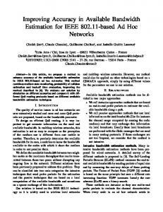
Figure 1: Interleaving of competing traffic and probing packets.. �� is the input gap, � is the probing packet length on the output link, � is the gap after interleaving with the competing traffic, ��� is the competing traffic throughput.
3 Single Hop Gap Model The idea behind using packet pairs to measure available bandwidth is to have the probing host send a pair of packets in quick succession and to measure how the gap between the two packets changes as a result of traversing the network (Figure 1). As the packets travel through the network, packets belonging to competing traffic will be inserted between them, thus increase the gap. As a result, the gap value at the destination host will be a function of the competing traffic rate, making it possible to estimate the amount of competing traffic. Unfortunately, how competing traffic affects the gap of a packet pair is much more complex than this description suggests. In the remainder of this section, we describe and evaluate a simple model that captures the relationship between the gap value and the competing traffic throughput for a single-hop network. JQR
Bc
go
gI
gB
0
DQR
Bo(1−r)
Bo*gI(1−r)
Q
Figure 2: Single hop gap model. The output gap � changes in two different ways: in the ����� region, � is not affected by ��� , while in the ����� region, � is proportional to ��� .
3
3.1 Single Hop Gap Model The gap model models the value of the output gap , i.e. the time between when the first bit of P1 and the first bit of P2 leave the router. The 3-D figure in Figure 2 shows the value of as a function of Q, the output queue size when packet P1 arrives at the router, and � � , the competing traffic for the time interval between the arrival of packets P1 and P2. �� is the gap value when P1 and P2 enter the router, and we call it input gap. Note that �� includes P1’s transmission delay 1 on the input link. � is the transmission delay of the probing packet on the output link. Since is also the gap value of two back-to-back probing packets on the bottleneck link, we call the bottleneck gap. Note that when the link capacity �� , the probing packet length, and �� are fixed,
and (defined as
� � ) in Figure 2 are constant. The model in Figure 2 assumes that we use FIFO queueing and that all probing packets have the same size. It also assumes that the competing traffic is constant between the arrival of packets P1 and P2; given that this input value is of the order of 1 msec, this is a reasonable assumption. We observe that the model has two regions. As we show below, the regions correspond to cases when the two packets P1 and P2 do or do not fall in the same queueing period. Queueing period is defined to be a time segment during which the queue is not empty; different queue periods are separated by a period when queue is empty. For this reason, we call the regions the Disjoint Queuing Region (DQR) and the Joint Queuing Region (JQR). In the DQR region, P2 will find an empty queue; this is directly result of the fact that P1 and P2 are in separate queueing periods and of our assumption that the competing traffic is constant for the P1-P2 period. In this situation, the output gap will be the input gap minus the queueing delay experienced by P1, i.e. . � ��
�
�
�
�
�
Under what condition will the queue be empty when P2 arrives? For that to happen, the router needs to complete three tasks before P2 arrives: process the queue � ( � � ), process P1 ( � ), and process the competing traffic that arrives between the probing packets ( � � � � ). The router has � time to complete these three operations, so the condition for operating in region DQR ��� � �� � , which is the triangular region labeled DQR in Figure 2. In this is � �� region, the output gap � does not depend on the competing traffic throughput ��� . Under all the other conditions, when P2 arrives at the router the queue will not be empty, i.e. P1 and P2 are in the same queueing period. This corresponds to the JQR region and the output gap consists of two time segments: the time to process P1 ( � ) and the time to process the competing traffic that arrives between the two probing packets ( � � � � ). So in this region, the output gap will be
��� � ��
� �� �� � �� ��
� �
� �� �
�� �
That is, in this region, the output gap � is a function of the competing traffic throughput ��� . This model directly points at a first problem in using packet pairs for estimating the competing traffic rates. If the packet pair happens to operate in the DQR region of the bottleneck router, the output will bear no relationship with the competing traffic and a user using the JQR equation (since the user does not know what region applies) will yield an arbitrary result. Furthermore, the estimate of the competing traffic obtained using a single packet pair will provide the average 1
Transmission delay is defined as the time for a packet to be placed on a link by a sender.
4
Ps
100Mbps
R1
10Mbps
R2
100Mbps
100Mbps
Pd
100Mbps
Cs
Cd
Figure 3: Testbed configuration for single hop network experiment.
competing traffic over � , which is a very short period. Since the competing traffic is likely to fluctuate, one will want to average the results of multiple samples, corresponding to independent packet pairs, but this increases the chance that some of the samples will fall in the DQR region. Note that these conclusions do not apply to packet train methods [8] [19], since the “pairs” that make up the a packet train are not independent. We discuss this further in Section 4.1.
3.2 Testbed Experiment To illustrate the gap model, we ran experiments on an isolated testbed. The testbed topology is shown in Figure 3. Ps and Pd are the probing source and destination, while Cs and Cd are used to generate competing TCP traffic. R1 and R2 are FreeBSD-based routers that run tcpdump on all relevant interfaces to record the packet timestamp information. We send out a probing train consisting of a series of evenly spaced 100B packets; each consecutive pair of packets in the train can serve as a probing pair. The competing traffic is generated using Iperf [22], which allows us to simulate typical user traffic such as FTP traffic. We can also control the competing traffic throughput by adjusting the TCP window size, which is useful in illustrating the features of the gap model. 3.2.1 Effect of JQR: capturing competing traffic
"
In this experiment, we use 1024 probing packets 2 and the input gap is set to 0.31 . We use a competing load of 7.2Mbps. A typical set of experimental results is shown in Figure 4; the top graph shows the output gap measured on R1 and the bottom graph shows the corresponding output gaps measured on R2. The increase in gap value on router R1 is caused by competing traffic on the bottleneck link. " (the time The increased gap values in the top graph of Figure 4 fall into three clusters: 1.2 " " to transmit a 1500B TCP competing packet on a 10Mbps link), 2.3 , and 3.8 . This is because these probing pairs are interleaved by exactly 1, 2, and 3 competing packets. The fact that at most " (note 3 packets are inserted in a probing gap should not be a surprise since the input gap is 0.31 that the input links are 10 times faster than the bottleneck link). Besides the increased gap values, " we also have some decreased gaps. Most of them are 0.08 , which is the transmission delay of the probing packet (100B) on the 10Mbps bottleneck link. The bottom graph shows that the increased gap values are maintained through router R2, because R2 has a higher output rate than input rate. 2
We use such a large number in order to get a large enough probing period, but we make sure it does not cause packet drops so as not to affect the competing flow’s throughput.
5
−3
4
x 10
input gap output gap Gap value (s)
3
2
1
0 380
390
400
410 420 430 Probing packet sequence number (R1)
440
450
−3
4
x 10
input gap output gap Gap value (s)
3
2
1
0 380
390
400
410 420 430 Probing packet sequence number (R2)
440
450
Figure 4: Effect of JQR. Input and output gap for routers R1 (top) and R2 (bottom). t1 input
t2 t3
output
*��
Figure 5: Competing packets at the input and output interface of R1. is the transmission * � � * � delay of the 3 competing packets on R1’s input link, is their transmission delay on the output * link, is the interval between the time when the first 3 packets finish transmission and the time when the second 3 packets arrive.
�
The observed changes in the gap values are a result of the burstiness of the competing traffic. In some cases, as is shown in Figure 5, the source Cs sends out three 1500B packets back-to-back *�� ( period in Figure 5). This builds up the queue in router R1 and the queue will drain during the *�� * period . After period , more competing traffic arrives. A packet pair that overlaps with period *�� will see an increased gap, corresponding to 1, 2, or 3 competing packets. A packet pair that falls *(� " *�� * in period will see its gap reduced to 0.08 . Packet pairs can also straddle the and periods, " " in which case their gap values reduce to values between � (0.08 ) and � (0.31 ). This effect corresponds to the DQR region, and in this experiment it is not very common.
6
−4
5
x 10
input gap output gap
Gap value (s)
4
3
2 400
410
420
430 440 450 460 470 Probing packet sequence number (R1)
480
490
500
Figure 6: Effect of DQR. The output gaps measured on router R1.
3.2.2 Effect of DQR: losing competing traffic We now change the competing traffic by setting the source TCP window size to 512B and the destination TCP window size to 128B. This forces the competing source to send one 128B packet each round trip time, i.e., the competing traffic is a low-bandwidth CBR load. The results in Figure 6 show that the increased gap values no longer cluster around a small set of discrete values. Instead, the output gap values take on a set of values fairly evenly distributed between about 2 and 4.3 msec. To explain this, we show a detailed snapshot of the starting and ending time of 2 competing packets (A and B) and 6 probing packets (1-6) in Figure 7 for both the input and output interfaces of router R1. The lines show the transmission delays of the packets 3 . Given the nature of the competing traffic, probing packets will always encounter an empty or very short queue. In some cases we see a gap increase because P2 is delayed (e.g. the gap for pair (2, " 3) increases to 0.414 ). In other cases P1 is delayed, and we end up in region DQR (e.g. pair (3, 4)). The delays experience by P1 or P2 correspond to the transmission time of a partial packet so they can take on any value.
3.3 Discussion The single hop gap model and our experiments show the challenges associated with using packet pairs to estimate competing traffic on the bottleneck link. To what degree the measured gap on the destination reflects the competing traffic load depends on what region the bottleneck router is operating in. The good news is that when we are operating in the right region, there is a proportional relationship between the output gap and the competing traffic. In the next section we will use this relationship to develop a new method for measuring the competing traffic. The bad news is that the 3
Because the time stamp recorded by tcpdump is the time the last bit of a packet passes through the network interface, for the segments in Figure 7, only the right end points are raw trace data. The left end points are calculated using packet length and the corresponding interface’s transmission rate. The small overlap between some of the packets, such as “3” and “A”, is not possible and is probably due to the timing error of tcpdump.
7
2
1
4
3
A
0
B
0.5 1 Time stamp at the input interface of R1 (s)
1
3
2
0.2
0.4
1.5 −3
x 10
4
A
0
6
5
5
6
B
0.6 0.8 1 1.2 Time stamp at the ouput interface of R1 (s)
1.4
1.6 −3
x 10
Figure 7: Snapshot of the interleaving between two competing packets and six probing packets. The top figure is the trace from the R1’s input interfaces, and the bottom figure is from R1’s output interface.
DQR region can introduce errors, so it is important to design the bandwidth probing experiments to avoid the DQR region.
4 Estimating Available Bandwidth We introduce a new method for estimating the competing traffic on the bottleneck link.
4.1 The IGI formula The experiments in Section 3.2.1 suggest a way of estimating competing throughput using packet trains instead of individual packet pairs. Note that the DQR effect is very small in this experiment, so there is a correlation between the increased gap values and the amount of competing traffic. gaps are inWe compute the competing traffic throughput as follows. Assume �� ��� � $� � ��
� � ; gaps are unchanged andprobing creased, the values are ��� they are represented � � � � $ � ��
� ; and � gaps decrease and they are denoted as ��� � �� � $ as �� � ��
� � . We use �� to denote the link capacity of R1, R2 � , i.e., the bottleneck link. Then � � � � . � is the amount of competing traffic that arrive at R1 during the probing period. ���
����
�
8
As a result, we can estimate the competing bandwidth on the bottleneck link as
� �� �
� �� �� � � � � . � � � �
�� � � � � � � � � �
�
(1)
This method of computing competing traffic load will be used by the IGI algorithm in Section 4.3, and we call it IGI formula. In this formula, the denominator is in general the length of the entire packet train. This is indeed the case when there are no out of order packets. When there are out of order packet, the gap involving the out of order packet are not valid and are excluded, thus reducing the denominator. For the experiments in Section 3.2.1, the IGI formula estimates a competing traffic throughput of 7.3Mbps. This compares well with the throughput of 7.2Mbps reported by Iperf. But IGI formula only works if we are in region JQR. When we apply the IGI formula to the experiments of Section 3.2.2, we obtain a throughput of 3.8Mbps, which is much higher than the real throughput of 1.4 Mbps.
4.2 Methodology A second part of our method is that we must control the measurements so that we use the JQR region. There are three parameters that we can control: 1. Probing packet size. Experiments with small probing packets are very sensitive to interference. The work in [8] also points out there can be significant post-bottleneck effects for small probing packet size. This argues for sending fairly large probing packets. 2. The number of probing packets. It is well known that the Internet traffic is bursty, so a short snapshot is not enough to tell the average traffic load. That argues for sending a fairly large number of probing packets. Note however that sending too many packets can cause queue overflow and packet loss and also increases the network load. 3. Initial probing gap. The single hop gap model in Figure 2 shows that increasing the input gap will increase the DQR area, where the output gap is independent of the competing traffic. � the DQR area does not even exist. This argues for using small input gaps. In fact, if � � , we are flooding the bottleneck link, which may cause packet loss However, when � and disrupt traffic. Our experiments show that our results are not very sensitive to the probing packet size and packet number and there is a fairly large range of good values for those two parameters. For example, a 700B packet size and 60 packets per train work well on the Internet. How to determine a good value for the initial probing gap is much more difficult. To clarify the trade-offs, imagine an experiment in which we send a sequence of packet trains with increasing initial probing gaps. For small initial probing gaps (smaller than , the transmission time on the bottleneck link), we are clearly flooding the network, and measurements will not provide any information on the available bandwidth. When the initial probing gap reaches , the DQR region appears in the gap model. Note that, unless the network is idle, we are still flooding the bottleneck link. So far, the average final output gap at the destination will be larger than the initial input gap. 9
When we continue to increase the initial probing gap, at some point, the average probing rate of the packet train will be equal to the available bandwidth on the bottleneck link. At that point, the final output gap will be equal to the initial input gap. This will continue to be the case as we continue to increase the initial probing gap, since all packets on average will experience the same delay. We believe that the initial input gap value for which the average final output gap is equal to the initial input gap is the right value to use for estimating the available bandwidth. That is the smallest initial input gap value for which we are not flooding the bottleneck link and hence we can expect to get the most accurate measurements. The IGI algorithm is based on this observation.
4.3 IGI Algorithm The IGI algorithm sends a sequence of packet trains with increasing initial packet gap. We monitor the difference between the average output gap and the input gap for each train and use the first train for which the two are equal. This point is called turning point. At this point, we use the IGI formula to compute the competing bandwidth. The available bandwidth is obtained by subtracting the estimated competing traffic bandwidth from an estimate of the bottleneck link bandwidth. The pseudo code of this algorithm is listed in Figure 8, and we call it Initial Gap Increasing (IGI) algorithm. In this algorithm, the bottleneck bandwidth can be measured using, for example, bprobe [6], nettimer [14], or pathrate [8]. Note that any errors in the bottleneck link capacity measurement will also affect the accuracy of the available bandwidth estimate. We will see an example in the next section. A key step in the IGI algorithm is the automatic selection of the turning point. We use the procedure GAP EQUAL() to do that. It tests whether the source gap “equals” the destination gap, where equality is defined as � �� �� �� . �� � * �� � �
� �� �� �� � �� � * �� � ��
�
In our experiments, � is set to 0.1.
5 Experiment and Analysis We implemented two versions of the IGI tool to accommodate the different network hosts we have access to: a kernel version for hosts on which we can change the operating system and a user-level version that can be run on any host. The kernel version sends out raw TCP packets as probing packets, and the timestamp is measured in the kernel with the help of libpcap [1] [17]. The user-level version uses UDP packets as probing packets, and the timestamp is the time when the probing application on the destination host receives the UDP packets. The kernel version has higher accuracy than the user-level version since it can get more accurate timestamps. Unless specifically mentioned, the measurements are carried out using the kernel version.
5.1 Testbed Experiment The experiments in this section are used to study the behavior of the IGI algorithm. The testbed topology used is the same as in Figure 3. 10
Algorithm IGI: �������
� ��
��������
S MALL G AP ; P ROBE N UM ; ��! �" PACKET S IZE ;
������
�� ������� �����
� ��
+ � �
� �
�
� ���� # ������$�
�����&%'�������
�����, .-/)
while 0 ! GAP ������� �����
EQUAL 0
+ ���
� �� 879 :�(�
� ��
� ��
� ���213� ���
��(�������
+ � �
�(�
����!>�?16�������
�����,
A � ��
� ���,
� ��
�����