Estimating Forest Structural Parameters Using Canopy Metrics ... - MDPI

Article

Estimating Forest Structural Parameters Using Canopy Metrics Derived from Airborne LiDAR Data in Subtropical Forests Zhengnan Zhang, Lin Cao * and Guanghui She Co-Innovation Center for Sustainable Forestry in Southern China, Nanjing Forestry University, Nanjing 210037, China; [email protected] (Z.Z.); [email protected] (G.S.) * Correspondence: [email protected] Received: 14 June 2017; Accepted: 6 September 2017; Published: 11 September 2017

Abstract: Accurate and timely estimation of forest structural parameters plays a key role in the management of forest resources, as well as studies on the carbon cycle and biodiversity. Light Detection and Ranging (LiDAR) is a promising active remote sensing technology capable of providing highly accurate three dimensional and wall-to-wall forest structural characteristics. In this study, we evaluated the utility of standard metrics and canopy metrics derived from airborne LiDAR data for estimating plot-level forest structural parameters individually and in combination, over a subtropical forest in Yushan forest farm, southeastern China. Standard metrics, i.e., height-based and density-based metrics, and canopy metrics extracted from canopy vertical profiles, i.e., canopy volume profile (CVP), canopy height distribution (CHD), and foliage profile (FP), were extracted from LiDAR point clouds. Then the standard metrics and canopy metrics were used for estimating forest structural parameters individually and in combination by multiple regression models, including forest type-specific (coniferous forest, broad-leaved forest, mixed forest) models and general models. Additionally, the synergy of standard metrics and canopy metrics for estimating structural parameters was evaluated using field measured data. Finally, the sensitivity of vertical and horizontal resolution of voxel size for estimating forest structural parameters was assessed. The results showed that, in general, the accuracies of forest type-specific models (Adj-R2 = 0.44–0.88) were relatively higher than general models (Adj-R2 = 0.39–0.77). For forest structural parameters, the estimation accuracies of Lorey’s mean height (Adj-R2 = 0.61–0.88) and aboveground biomass (Adj-R2 = 0.54–0.81) models were the highest, followed by volume (Adj-R2 = 0.42–0.78), DBH (Adj-R2 = 0.48–0.74), basal area (Adj-R2 = 0.41–0.69), whereas stem density (Adj-R2 = 0.39–0.64) models were relatively lower. The combination models (Adj-R2 = 0.45–0.88) had higher performance compared with models developed using standard metrics (only) (Adj-R2 = 0.42–0.84) and canopy metrics (only) (Adj-R2 = 0.39–0.83). The results also demonstrated that the optimal voxel size was 5 × 5 × 0.5 m3 for estimating most of the parameters. This study demonstrated that canopy metrics based on canopy vertical profiles can be effectively used to enhance the estimation accuracies of forest structural parameters in subtropical forests. Keywords: forest structural parameter; LiDAR; canopy metric; canopy vertical profile; subtropical forest

1. Introduction Forested ecosystems are spatially dynamic and continuously changing and therefore comprise complex and heterogeneous forest structures [1,2]. Forest structure, defined as the spatiotemporal arrangement of structural components in specific vertical and horizontal spatial patterns within a forest stand [3–5], is recognized as both a product and driver of forest biophysical processes [6] and Remote Sens. 2017, 9, 940; doi:10.3390/rs9090940

www.mdpi.com/journal/remotesensing

Remote Sens. 2017, 9, 940

2 of 26

represents important forest information, which is useful for guiding multi-functional forest management [7]. Forest structural parameters (e.g., tree height, volume, biomass or stem density etc.) provide considerable information on the spatial and temporal distribution of forests as well as structural properties, and are considered critical components of forest inventory [8] and reliable diversity indicators across forest successional stages [3]. So obtaining spatially continuous estimates of forest structural parameters is valuable for supporting long-term sustainable forest management [9]. Subtropical forests are distributed in a transition zone between tropical and temperate zones, i.e., the region lying largely from 23.5° to 40° latitude in the northern or southern hemispheres [10]. Subtropical forests consist of both subtropical humid and subtropical dry forests, which have unique ecological characteristics when compared to tropical and temperate regions [11]. Subtropical forests, which account for approximately 9% of the world’s forest area [12], are considered a carbon sink contributing to global forest carbon sequestration, and have high species richness, complex structure of forest, high biodiversity and high net ecosystem productivity (NEP) [11]. Quantitative measurements of forest structural parameters of subtropical forests are required to understand forest ecological mechanisms, promote regional ecological developments, maintain biodiversity and enhance regional carbon balance [13]. Traditionally, forest structural parameters are assessed by conventional field inventories, which is time-consuming, costly and limited in spatial extent [2,14]. As a promising earth observation technique, remote sensing has shown great potential for providing multi-scale, multi-dimensional and multi-temporal earth surface information [15] for instantaneous, quantificational and accurate measurements of spatially continuous wall-to-wall properties of forest structure over large-scale areas in lieu of time-consuming and labor-intensive inventory [16]. Furthermore, integrating information from remotely sensed data with a high level of precision and temporal consistency has been recognized as having the ability to describe forest biophysical properties and effectively enhance the performance of forest structure estimations [17]. Estimates of forest stand structural parameters have been derived from optical remote sensing data for several decades [17,18]. However, passive remote signals are generally reflected or absorbed in the uppermost canopy layers and tend to “saturate”, especially in dense forest(i.e., high canopy closure), limiting the ability to characterize vertical structure [19,20]. Similarly, Radar (Radio Detection and Ranging) technology also reveals the aforementioned data saturation problems, due to noise introduced by terrain, surface moisture and other factors [20,21]. Conversely, as a promising active remote sensing technology, Light Detection and Ranging (LiDAR) can be used to directly estimate a spatially explicit three-dimensional (3D) canopy structure with submeter accuracy by transmitting short laser pulses and receiving returned signals [22,23]. Furthermore, LiDAR systems have the ability to overcome the data saturation problems in optical or Radar remote sensing, as a laser beam can strongly penetrate through even dense and multilayered forest canopies to the earth’s surface [24]. Means et al. (2000) [25] estimated forest structural parameters, i.e., tree height, basal area, and volume, using airborne LiDAR data over a Douglas-fir-dominated temperate forest in the Western Cascades of Oregon. They found that the estimation of tree height predicted by the metrics of height percentiles and resulted in R2 values of 0.93–0.98. The R2 values were 0.94–0.95 and 0.95–0.97 for basal area and volume, which were predicted using the metrics of height percentiles and canopy densities as independent variables. Silva et al. (2016) [26] predicted and mapped volume using LiDAR metrics in Eucalyptus plantations in tropical forests (located in São Paulo, Brazil), and found that volume (Adj-R2 = 0.84) was well predicted by the coefficient of variation of return height and the 99th height percentile from LiDAR. Tesfamichael and Beech (2016) [27] used height-related metrics (e.g., height percentiles, maximum height) and canopy density metrics to estimate plot-level structural attributes (i.e., mean height, maximum height, crown diameter and aboveground biomass) over a savanna ecosystem region located in the south western part of Zambia, and resulted in R2 values of 0.48–0.95. However, these studies often include height and density predictors with little physical justification for model formulation. Moreover, they usually neglected a mechanism to summarize complex canopy characteristics into simple parameters, which can potentially be used for estimates of forest


3 of 26

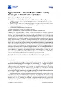
structural parameters in different forest conditions [14,28], and the standard metrics (i.e., heightbased and density-based metrics) tend to be strongly inter-correlated, and depend on forest conditions, plot sizes, point cloud density and geometrical distributions of point clouds etc. [29–33], and a large subset of these metrics are linked to only a few forest stand characteristics. Thus, these metrics generally have a relatively low transferability and are limited in describing the vertical heterogeneity of forest structure [24]. Canopy vertical profiles, defined as the distributed curves about the characteristic of forest structural components as a function of height above ground, are intimately linked to the vertical distributions of forest structural elements (e.g., foliage, branches, trunks etc.), and have strong potential in enhancing the theoretical explanations of vertical forest structure [4,34,35]. Canopy vertical profiles are important descriptors of forest structure. Lefsky et al. (1999) [36] developed an approach termed “canopy volume models (CVM) ” to characterize three-dimensional (3D) volumetric structure of forest canopies by quantifying the differences in the total volume and spatial organization of the tree foliage, and this approach is beneficial to distinguish specific volumetric canopy architecture. They found relatively high accuracies (R2 = 0.52–0.91) for estimating forest structural parameters using the metrics derived from canopy vertical profiles (i.e., canopy volume profiles (CVP) and canopy height profiles (CHP)). Lovell et al. (2003) [37] used airborne and terrestrial LiDAR data to derive foliage profiles (FP) and estimated effective leaf area index (LAI) in temperate forests located in southern Australia. They found that results compared with LAI derived from classified hemispherical photographs with agreement within 8%. Coops et al. (2007) [38] refined the CVM approach to adapt discrete return LiDAR data. In addition, a Weibull fitting approach was conducted to fit FP profiles and further obtain relevant LiDAR metrics, and finally a number of forest structural parameters (i.e., mean height, basal area) (R2 = 0.65–0.85) were estimated. Hilker et al. (2010) [39] assessed and compared canopy metrics derived from canopy vertical profiles using airborne and terrestrial LiDAR data. The results showed that airborne and terrestrial LiDAR were both able to accurately determine canopy height (absolute error of height was less than 2.5 m) and LAI (R2 = 0.86– 0.90). However, most previous studies that estimate forest structural parameters using canopy metrics derived from canopy vertical profiles were conducted in temperate, tropical and boreal forests, and published studies of the subtropical forests are few. In this study, the standard metrics and canopy metrics derived from airborne LiDAR data are used to estimate plot-level forest structural parameters (i.e., mean diameter at breast height, Lorey’s mean height, stem density, basal area, volume, and aboveground biomass) individually and in combination over a north subtropical secondary forest in southern Jiangsu Province, China. The objectives of this study are: (1) to derive two suites of canopy metrics, i.e., canopy volume (CV) metrics and Weibull-fitted (WF) metrics, using voxel-based CVM and Weibull fitting approaches separately; and (2) to assess the capability of standard metrics and canopy metrics based models and combination models for estimating forest structural parameters and to evaluate the accuracies of the models; and (3) to explore the optimal horizontal and vertical resolution of voxels for the predictive models. 2. Materials and Methods An overview of the workflow for calculating plot-level forest structural parameters estimation is shown in Figure 1. Firstly, a 1-m Digital terrain model (DTM) was created by the last return points. The data was filtered to remove the above-ground returns, and then the DTM was created by calculating the average elevation from the remaining (ground) LiDAR returns within a cell. Cells that contain no points are interpolated by neighboring cells. The point cloud was then normalized against the ground surface height. Secondly, standard metrics (i.e., height-based (HB) metrics and densitybased (DB) metrics) and canopy metrics (i.e., canopy volume (CV) metrics and Weibull-fitted (WF) metrics) were extracted. The suite of canopy volume (CV) metrics was derived by a voxel-based CVM approach, and another suite of WF-metrics was derived by calculating α (scale) and β (shape) parameters of Weibull function fitting to canopy height distribution (CHD) and FP. Thirdly, the estimation capability of standard metrics-based (SM) models, canopy metrics-based (CM) models


4 of 26

and combination models were examined for estimating forest structural parameters separately. Finally, the accuracies of the models were assessed and validated by field measured data.

Figure 1. An overview of the workflow for forest structural parameters estimation. DTM: Digital Terrain Model.

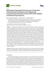
2.1. Study Area This study was conducted in Yushan Forest, a state-operated forest and national park located near the town of Changshu in Jiangsu Province, southeastern China (120°42′9.4″E, 31°40′4.1″N). The total site area is approximately 1260 ha, which covers approximately 1140 ha of forests. Topographically, the site’s mountain terrain extends from northwest to southeast and the ridge line is more than 6500 m, with the elevation range between approximately 20 and 261 m above sea level. This site is situated in the north-subtropical monsoon climatic region with an annual mean temperature of 15.4 °C, and precipitation of 1047.7 mm, and annual mean relative humidity of approximately 80%. The highest monthly precipitation occurs from June to September. The soil type in Yushan is composed mainly of mountain yellow-brown earth. The forest in Yushan belongs to the north-subtropical mixed secondary forest with three main forest types: conifer-dominated, broadleaved dominated and mixed forests. The dominant broad-leaved tree species include Oriental oak (Quercus variabilis Bl.), Chinese sweet gum (Liquidambar formosana Hance) and Sawtooth oak (Quercus acutissima Carruth.) of deciduous broad-leaved trees species, mixed with other evergreen broadleaved tree species including Camphorwood (Cinnamomum camphora (L.) Presl.) and Chinese holly (Ilex chinensis Sims.). The primary coniferous forests are dominated by evergreen coniferous tree species, including Masson pine (Pinus massoniana Lamb.), Chinese fir (Cunninghamia lanceolata (Lamb.) Hook.), slash pine (Pinus elliottii Engelm.) and Japanese Blackbark Pine (Pinus thunbergii Parl.). Figure 2 shows an overview of the study site and distribution of sample plots and Figure 3 shows the field photos of three forest types.


5 of 26

Figure 2. Study site and distribution of sample plots.

Figure 3. Examples of the three main forest types in study site. (a) Coniferous forest; (b) broad-leaved forest; (c) mixed forest.

2.2. Data Acquisition and Pre-Processing 2.2.1. LiDAR Data Small footprint airborne LiDAR data were acquired on 17 August 2013 using a Riegl LMS-Q680i sensor flown at 900 m above ground level, with a flight speed of 55 m·s−1 and a flight line side-lap of ≥60%. The sensor recorded returned waveforms of laser pulse with a temporal sample spacing of 1 ns (approximately 15 cm). The LiDAR system was configured to emit laser pulses in the near-infrared band (1550 nm) at a 360 kHz pulse repetition frequency and a 112 Hz scanning frequency, with a scanning angle of ±30° from nadir and a swath of 1040 m. The dataset had an average beam footprint size of 0.45 m (nadir) in diameter. The average ground point distances of the dataset were 0.49 m (flying direction) and 0.48 m (scanning direction) in a single strip, with pulse density of approximately 5.06 pulse m−2. The final extracted point clouds and associated waveforms were stored in LAS 1.3 format (American Society for Photogrammetry and Remote Sensing, Bethesda, MD, USA). In order to obtain the relative height of trees, raw point cloud data were first filtered by removing outliers. The data were filtered to remove non-ground points using an algorithm adapted from Kraus


6 of 26

and Pfeifer (1998) [40], which was based on a method of linear least-squares interpolation, and then the data were smoothed by the median filter (moving square windows of size 5 × 5 m). After filtering the non-ground points, a 1-m Digital terrain model (DTM) was created by calculating the average elevation from the ground points within a cell (cells that contain no points were filled by interpolation using neighboring cells). Then, the point cloud was then normalized against the ground surface height and extracted for each plot. Point clouds for all plots (n = 51) were finally extracted using the coordinates of the lower left and upper right corners. 2.2.2. Field Data The field data for the study site were collected from June to August in 2012 and in August of 2013. Throughout the Yushan study region, a total of 51 square sample plots (30 × 30 m) were established, covering the forest type, dominant species compositions, age classes, and site indices, according to an historical forest resource inventory data (2012). All plots were divided into broadleaved forest (n = 14), coniferous forest (n = 14), and mixed forest (n = 23). The centers of each plot and plot corners were located using Trimble GeoXH6000 Handheld GPS (Trimble, Sunnyvale, CA, USA) units equipped with a dual frequency GNSS antenna, and corrected with high precision real-time differential signals received from the Jiangsu Continuously Operating Reference Stations (JSCORS), resulting in a submeter positional of accuracy of less than 0.5 m [41]. The plot directions and inclined angles were recorded by forest compass, and the border lengths were measured by PI tape. For all live trees with a diameter at breast height (DBH) over 5 cm, tree type, diameter, height, height to crown base, crown width in both cardinal directions, crown class, and crown transparency were measured. DBH was measured on all trees using a diameter tape. Heights of all trees were measured using a Vertex IV hypsometer (Haglöf, Långsele, Sweden). Crown widths were obtained by measuring the average of two values measured along two perpendicular directions from the location of the tree top. In addition, small trees (DBH < 5 cm) and dead wood were also tallied for total stem density, but not used in biomass calculations. Several forest structural parameters were assessed in this study, including mean DBH, Lorey’s mean height (i.e., the basal area weighted height), stem density, basal area, volume and aboveground biomass. In addition, aboveground biomass of each tree was calculated by means of the species specific allometric equations from local or nearby province [42–47] (Table A1), and the tree-based calculation results were summed within each plot to determine plot-level forest aboveground biomass. Plot-level volume was similarly calculated using provincial species specific volume equations of individual trees, which were based on DBH as predictor variables. A summary of plotlevel forest structural parameters data is presented in Table 1. Table 1. A summary of plot-level forest structural parameters data. Parameters DBH/cm hLorey/m N/(ha−1) G/(m2·ha−1) V/(m3·ha−1) AGB/(Mg·ha−1)

Coniferous Forest (n = 14) Range Mean SD 8.08–19.22 12.62 2.53 4.47–12.97 9.50 2.00 656–3167 1690.64 643.15 6.97–34.07 23.08 6.79 32.19–178.08 116.53 34.75 11.02–127.39 69.74 27.76

Broad-Leaved Forest (n = 14) Range Mean SD 11.63–20.99 15.32 3.29 7.70–18.52 11.35 2.75 322.00–1833.00 1126.00 428.55 12.11–28.10 21.92 3.89 90.62–212.45 132.77 32.30 32.03–219.67 94.28 44.93

Mixed Forest (n = 23) Range Mean SD 10.58–19.69 13.90 2.51 7.79–14.18 10.79 1.71 689.00–2344.00 1431.78 438.40 16.84–35.37 23.98 4.46 82.78–187.91 131.98 28.67 49.65–141.73 89.36 25.95

Notes: DBH: Mean diameter at breast height; hLorey: Lorey’s mean height; N: Stem density; G: Basal area; V: Volume; AGB: Aboveground biomass.

2.3. Derived Metrics 2.3.1. Canopy Volume Model Approach A voxel-based CVM approach was applied for point cloud data to derive metrics in this study. The canopy spaces were first organized as a matrix composed of voxels (5 × 5 × 0.5 m3), and these voxels were classified as either “filled” or “empty” volume depending on the presence or absence of


7 of 26

LiDAR points within each voxel. “Filled” voxels were further classified as either “euphotic“ zone, if they were located in the uppermost 65% of all filled voxels, or as “oligophotic” zone if they were located below the point, whereas “empty” voxels were located either below (“closed gap”) or above the canopy (“open gap”) [38]. Open gap, euphotic, oligophotic and closed gap were determined as four canopy structure classes, with units defined as the volume of each class per unit area. All volume elements (Open gap, Oligophotic, Euphotic, Closed gap, Filled, Empty) were derived as canopy volume (CV) metrics using the CVM method and canopy volume profile (CVP) was visualized. Figure 4 shows the illustration of voxel-based CVM approach. Point clouds of a plot (30 × 30 m2) were voxelized, and divided into 36 vertical columns of voxels, and each column was further stratified with four canopy structure classes. All columns of a plot were expanded in a panel and the canopy volume distribution (CVD) was presented (Figure 4c). Finally, the volume percentages of canopy structure classes of each height interval (0.5 m) were calculated, resulting in CVP (Figure 4d). Notably, an appropriate voxel volume size for CVM in this study was been considered because various voxel sizes likely change the distributions and proportions of canopy structure classes. Thus, this study also investigated the influence of various voxel sizes on the accuracies of the models. Given the average beam footprint size of 0.45 m, average ground point distances of 0.49 m (flying direction) and 0.48 m (scanning direction) and pulse density of approximately 5.06 pulse·m−2, horizontal resolutions of 1 m to 10 m were chosen (which were multiples of the footprint size and average ground point distances). Vertical resolutions of 0.5 m and 1 m were chosen to correspond to roughly three and six sampling intervals of the returned waveform. A sensitivity analysis was performed using CV-metrics (i.e., Open gap, Oligophotic, Euphotic, Closed gap, Filled, Empty).

Figure 4. The illustration of voxel-based canopy volume model. (a) A plot (30 × 30 m2) was stratified with voxelization and height bin is 0.5 m; (b) a voxel column was stratified in four structure classes (open gap, euphotic, oligophotic, closed gap) with canopy volume model approach; (c) canopy volume distribution, which shows the distribution of canopy structure classes after all columns were expanded in a panel; (d) the canopy volume profile, which was transformed from the canopy volume distribution diagram, shows the volume percentage of each class of total volume in each height interval.

2.3.2. Weibull Fitting Approach Canopy height distributions (CHD), which describe vertical distributions of foliage elements and non-photosynthetic tissues within canopy spaces, were used to measure the distribution of laser returns within the 0.3-m bins (i.e., a 30 × 30 × 0.3 m3 rectangular section) from the ground to canopy top [48,49]. In this study, a two-parameter Weibull density function (PDF) was used to describe CHD on each plot. As a Weibull model is highly adaptive, ranging from an inversed J-shape to unimodal skewed and unimodal symmetrical curve, the Weibull model has flexibility in characterizing distributions of a range of forest attributes [50,51]. The two parameters, i.e., Weibull scale (α1) and


8 of 26

Weibull shape (β1), were derived by the maximum likelihood estimation method. Weibull scale determines the basic shape of the distribution density curve and Weibull shape controls the breadth of the distribution [52]. Foliage profile (FP) can delineate the vertical distribution of canopy phytoelement (e.g., leaf, stem, twig, etc.) density above the ground within a forest stand [37]. FP is defined as the total one-sided leaf area that is involved in photosynthesis per unit canopy volume at canopy height z, and describes changes in the leaf area distribution with increasing height [53]. FP is highly related to leaf area index (LAI), which was demonstrated in previous studies [35,54], and the relationship between FP and LAI is: z2

L ( z ) =  FP ( z ) dz ,

(1)

z1

where L(z) is the cumulative leaf area index (LAIc) from the ground to a given height z; FP(z) represents the foliage area volume density at height z (is the vertical foliage profile in a thin layer or “slice” through a canopy as a function of height z); z1 and z2 are different canopy height. A height interval or each vertical “slice” was 0.3 m. Meanwhile, we assumed that foliage elements in a thin “slice” were very small so that occlusion can be neglected, and leaves presented Poisson random distribution. Because airborne LiDAR is incapable of resolving foliage angle distribution, clumping and non-foliage elements, the foliage profiles derived from airborne LiDAR are referred to here as “apparent” foliage profiles and effective LAI [37]. In this study, LAI can be indirectly determined from LiDAR by estimating the derived gap probability in the canopy [37,38], and the gap probability be estimated as the total number of laser hits up to a height z relative to the total number of LiDAR shots as follows:

 (# z j | z j > z )  , L (z ) = −ln (Pgap (z )) = −ln  1 −   N  

(2)

where Pgap (z) is a gap probability measurement at height z, #z is the number of hits down to a height z above the ground, and N is the total number of shots emitted up to the sky. Previous studies have showed that Weibull distribution function can also delineate vertical foliage profiles distributions [37,55]. In this study, the Weibull fitted scale parameter (α2) and shape parameter (β2) were derived from the apparent FP by linking Weibull cumulative function to cumulative projected foliage area index [37,38]:

 −  1− z / H max   α2  L( z ) = 1 −  e   

β2

 ,   

(3)

where α2 and β2 are fitted parameters, z is the height, and H is the maximum height in a plot. Moreover, another suite of standard metrics were calculated, including height-based (HD) metrics (h25, h50, h75, h95, hmean, hcv, hskewness and hkurtosis) and density-based (DB) metrics (d1, d3, d5, d7, d9, CC2m). A summary of these metrics with corresponding descriptions is shown in Table 2.


9 of 26

Table 2. The description of LiDAR canopy metrics. LiDAR Metrics

Height-based

Density-based

Canopy volume

Weibull-fitted

Description Standard metrics The percentiles of the canopy height distributions Percentile heights (h25, h50, h75 and h95) (25th, 50th, 75th and 95th) of first returns. Mean height (hmean) Mean height above ground of all first returns. Coefficient of variation of heights (hcv) Coefficient of variation of heights of all first returns. Skewness and Kurtosis of heights The skewness and kurtosis of the heights of all points. (i.e., hskewness and hkurtosis) The proportion of points above the quantiles Canopy return density (d1, d3, d5, d7 and d9) (10th, 30th, 50th, 70th and 80th) to total number of points. Canopy cover above 2 m (CC2m) Percentages of first returns above 2 m. Canopy metrics Filled and Empty zones of CVM The voxels contained point clouds and voxels contained (i.e., Filled and Empty) no point clouds within canopy spaces. Open and Closed gap zones of CVM The empty voxels located above and below the canopy (i.e., Open gap (OG) and Closed gap (CG)) respectively. The voxels located within an uppermost percentile (65%) Euphotic and Oligophotic zones of CVM of all filled grid cells of that column, and voxels located (i.e., Euphotic (Eu) and Oligophotic (Oligo)) below the point in the profile The scale parameter α and shape parameter β of the α1 and β1 parameter of Weibull distribution Weibull density distribution fitted to CHD. The scale parameter α and shape parameter β of the α2 and β2 parameter of Weibull distribution Weibull density distribution fitted to FP.

2.4. Metrics Selection and Statistical Analysis All of the LiDAR metrics in Table 2 were used to analyze pair-wise relationships among different forest structural parameters (DBH, Lorey’s mean height, stem density, basal area, volume and AGB) by Pearson’s correlations (r). Then the metrics with low correlations (r < 0.2) were excluded and candidate metrics were used in the regression analysis. In the multiple regression analysis, all of the dependent variables and independent variables were transformed using the natural logarithm to improve linearity and corrected for bias using a bias correction factor (BCF) [56]. Some studies have applied log transformations to both dependent variables and independent variables for estimations of forest parameters [57,58]. Multiple regression models including forest type-specific (coniferous forest, broad-leaved forest, and mixed forest) models and general models of all plots were then established. Both stepwise variable selection and the maximum coefficient of determination (R2) improvement variable selection techniques were applied to select the metrics to be included in the models [59]. Independent variables were left in the model using an F-test with a p < 0.05 significance level. The standard least-squares method was used [60]. To ensure that the independent variables were not highly correlated, multicollinearity was evaluated using Principal Component Analysis (PCA) based on the correlation matrix. Models with condition number (k) lower than 30 were accepted to ensure that there was no serious multicollinearity in the selected models [57]. The best fitting models were then selected based on the lowest Akaike information criterion value [61]. The accuracies of predictive models were evaluated using adjusted coefficient of determination (Adj-R2), Root-Mean-Square Error (RMSE), which has been transformed back to original scale, and relative RMSE (rRMSE), which are defined as the percentage of the ratio of RMSE and the observed mean values. In this study, dummy variables (or class variables) were added to the selected models as the dependent variables to assess whether these models differ between forest types [62]. Once the best models were chosen, leave-one-out crossvalidation was performed to evaluate the predictive accuracies of the models [63].

Adj-R2 = 1 − RMSE =

n −1 (1 − R2 ) n − p −1 1 n ( x i − xˆi )2 n i =1

(4)

(5)


10 of 26

rRMSE = where x

i

is the observed value for plot i,

RMSE × 100% , x

x

is the observed mean value for plot i, xˆ i

(6)

is the

estimated value for plot i, n is the number of plots i, and p is the number of variables. 3. Results 3.1. Profile Analysis The plots of each forest type were stratified into three groups (low, medium, and high), according to the Lorey’s mean height from low to high. In each group, three plots were selected, and a total of nine typical plots were selected. For the typical plots, CVD, CVP and FP were extracted, as shown in Figures 5–7. In addition, Figure 8 shows the mean LAIc for plots in different forest types and mean CVD. Figure 5 shows the spatial arrangements of four canopy structure classes for coniferous, broadleaved, and mixed forest plots. Generally, Oligophotic zones were larger than euphotic zone in filled volume; coniferous forests had the largest open gap zone and the smallest closed gap zone, whereas broad-leaved forests plots had a larger and wider spread of closed gap zone than mixed forest. Similarly, the percentage of closed gap volume was larger in broad-leaved forests than in mixed forests, and the lowest percentage of closed gap volume was in coniferous forests (Figure 6). The mean CVPs (Figure 6d,h,l) show that the percentages of open gap volume were the highest in coniferous forests, and the differences were not significant between the percentages of open gap volume in broad-leaved forests and mixed forests. The percentages of filled volume in coniferous and mixed forests were significantly higher than in broad-leaved forest, and the differences for the percentage of filled volume between coniferous and mixed forest were not significant.

Figure 5. Canopy volume distributions for the plots in different forest types. (a–c) Three typical plots of coniferous forest; (d–f) three typical plots of mixed forest; (g–i) three typical plots of broad-leaved forest.


11 of 26

Weibull models were fitted to canopy foliage distribution and matched the shape of foliage profile relatively well (Figure 7). In general, the FP profiles first exhibited a strong increasing trend, followed by a decreasing trend. Particularly, the peaks of FP in coniferous and mixed forests occurred in the lower or middle portions of the canopies whereas the peaks of broad-leaved forests were distributed more toward middle and upper portions of the canopies. Comparing with the mean foliage profiles and Weibull curves of three forest types, the curve showing the spatial distribution of FP values was smoother in broad-leaved forests than those of coniferous or mixed forests. The Weibull shapes of mixed forest canopy were slightly steeper than those of coniferous forest stands, indicating a wider spread of foliage within the canopy (Figure 7d,h,l). This same trend can be seen in the mean CHDs (Figure 8b–d). The mean LAIc values below the threshold of 12 m (approximately middle canopy) were relatively high for mixed forests, followed by coniferous forests and broad-leaved forests (Figure 8a). Above the tree height of 12 m, the increasing slope of the mean LAIc of the broad-leaved forests with increasing tree height was higher than that of coniferous forests, and maintained a relative high increasing trend, whereas the increasing trend of coniferous forests and mixed forests gradually tended to saturate. As a result, the mean LAIc value of broad-leaved forests was eventually higher than that of mixed forests, and lowest for coniferous forests.

Figure 6. Canopy volume profiles for the plots in different forest types. (a–c) Three typical plots of coniferous forest; (e–g) three typical plots of mixed forest; (i–k) three typical plots of broad-leaved forest; (d,h,l) the mean canopy volume profiles in each forest.


12 of 26

Figure 7. Foliage profiles for the plots in different forest types. (a–c) Three typical plots of coniferous forest; (e–g) three typical plots of mixed forest; (i–k) three typical plots of broad-leaved forest; (d,h,l) the mean foliage profiles in each forest type.

Figure 8. The mean cumulative leaf area index profiles for plots in different forest types (a) and mean canopy height distribution: (b) coniferous forest; (c) mixed forest; (d) broad-leaved forest.

3.2. Accuracy Assessments The selected metrics and accuracy assessment results of all the multi-regression models (i.e., SM models, CM models, and combination models) are shown in Tables A1–A3 and Table 3 summarizes their accuracies. All of the forest structural parameters were generally well estimated (Adj-R2 = 0.39– 0.88, rRMSE = 5.13–29.86%). Overall, Lorey’s mean height (Adj-R2 = 0.61–0.88, rRMSE = 5.13–12.79%) and AGB (Adj-R2 = 0.54–0.81, rRMSE = 12.19–28.42%) was predicted most accurately. For volume,


13 of 26

DBH and basal area, the R2 values were slightly lower and ranged from 0.42 to 0.78, 0.48 to 0.74 and 0.41 to 0.69, respectively. The lowest accuracy was found for stem density (Adj-R2 = 0.39–0.64, rRMSE = 18.68–29.86%). In comparison, most of forest structural parameters in type-specific models (Adj-R2 = 0.44–0.88, rRMSE = 5.13–28.42%) had higher accuracies than in general models (Adj-R2 = 0.39–0.77, rRMSE = 8.54–29.86%), indicating that the accuracies of forest type-specific models were generally improved rather than general models. Furthermore, the fitted models of the forest structural parameters were relatively more accurate for coniferous forests (Adj-R2 = 0.54–0.81, rRMSE = 8.59– 26.55%) than broad-leaved forests (Adj-R2 = 0.50–0.88, rRMSE = 6.39–28.42%) and mixed forests (R2 = 0.44–0.84, rRMSE = 5.13–29.52%). Compared with canopy metrics based models (Adj-R2 = 0.39–0.83, rRMSE = 6.94–29.26%), standard metrics based models had a relatively higher performance (Adj-R2 = 0.42–0.84, rRMSE = 5.60–29.86%) and the combination models performed best (Adj-R2 = 0.45–0.88, rRMSE = 5.13–28.96%), indicating the inclusion of canopy metrics potentially improved the estimation performances of structural parameters. For all of the general SM models, the standard metrics that were regressed against for fitting models included most of the standard metrics, indicating those had a relatively strong correlation with forest structural parameters. Overall, h95 (selected by four out of six models), d7 (selected by four out of six models), d3, hcv and d9 (each of them was selected by three out of six models) were the most frequently selected, indicating these metrics are more sensitive and representative to the forest structural parameters. For general CM models, all of CV metrics and WF metrics were selected for estimating forest structural parameters. Within CV metrics, the statistic of Oligophotic (all selected by six models), Empty (selected by four out of six models) and Open (selected by four out of six models) were sensitive to forest structural parameters and these metrics were selected both in the general models and forest type-specific models, suggesting that the three metrics have a strong ability to explain variations. Within WF metrics, α1 was relatively sensitive to structural parameters (selected two out of six models). In six general combination models, most of standard metrics (nine out of 14) and canopy metrics (four out of total 10) were used in combination for parameter estimations. The metrics of Oligophotic, Empty, h95 remained sensitive to structural parameters (selected by 2–4 out of six general combo models). Moreover, h75, d1 and β1 (selected by 2–3 out of 6) became more sensitive for DBH, Lorey’s mean height, and stem density in combination models than SM models. Figure 9 shows the LiDAR estimated versus the field measured forest structural parameters as well as the results for cross-validation in all plots models based on standard metrics and canopy metrics. As indicated, Lorey’s mean height and AGB models were fitted best and resulted in R2 values of 0.79 and 0.66, followed by DBH (R2 = 0.60), volume (R2 = 0.60) and basal area (R2 = 0.52), whereas the accuracy of stem density model was the lowest (R2 = 0.49). For Lorey’s mean height, AGB, DBH, and volume estimations, their relationships were close to the 1:1 line whereas basal area and stem density had a relationship that deviated from the 1:1 line, with a slightly larger deviation in broadleaved forests.


14 of 26

Table 3. A summary of selected metrics and accuracy assessment results of predictive models. Forest Types

All plots

Coniferous forest

Broad-leaved forest

Mixed forest

Parameters DBH/cm hLorey/m N/(ha−1) G/(m2·ha−1) V/(m3·ha−1) AGB/(Mg·ha−1) DBH/cm hLorey/m N/(ha−1) G/(m2·ha−1) V/(m3·ha−1) AGB/(Mg·ha−1) DBH/cm hLorey/m N/(ha−1) G/(m2·ha−1) V/(m3·ha−1) AGB/(Mg·ha−1) DBH/cm hLorey/m N/(ha−1) G/(m2·ha−1) V/(m3·ha−1) AGB/(Mg·ha−1)

Standard Metrics h95, d1, d7 hcv, h95, d7, d9 hcv, d1, d7, d9 h95, d3, d7 hcv, h25, h50, d3 hkurtosis, h95, d3, d9 h95, d1, d7 hcv, h95, d7, d9 hcv, d1, d7, d9 h95, d3, d7 hcv, h25, h50, d3 hkurtosis, h95, d3, d9 h95, d1, d7 hcv, h95, d7, d9 hcv, d1, d7, d9 h95, d3, d7 hcv, h25, h50, d3 hkurtosis, h95, d3, d9 h95, d1, d7 hcv, h95, d7, d9 hcv, d1, d7, d9 h95, d3, d7 hcv, h25, h50, d3 hkurtosis, h95, d3, d9

SM Models Adj-R2 RMSE 0.60 *** 1.72 0.75 *** 0.97 0.42 *** 423.75 0.44 *** 3.99 0.46 *** 22.34 0.64 *** 19.17 0.67 ** 1.20 0.66 1.09 0.60 315.78 0.62 ** 4.53 0.69 ** 22.40 0.72 ** 16.86 0.61 ** 1.70 0.84 *** 0.78 0.60 298.99 0.54 2.62 0.56 19.49 0.57 26.80 0.48 ** 1.66 0.81 *** 0.60 0.48 ** 336.73 0.45 ** 3.08 0.60 *** 16.76 0.64 *** 13.20

rRMSE % 12.33 9.15 29.86 17.23 17.46 22.47 9.50 11.47 18.68 19.63 19.22 24.17 11.12 6.91 26.55 11.96 14.68 28.42 11.94 5.60 28.52 12.86 12.70 14.77

CM Models Canopy Metrics Adj-R2 OG, Oligo, Empty, β2 0.50 *** Oligo, Filled, Empty, α1 0.61 *** OG, Eu, Oligo, β1 0.39 *** Oligo, Empty, α2 0.41 *** OG, Eu, Oligo, α1 0.42 *** OG, Oligo, CG, Empty 0.54 *** OG, Oligo, Empty, β2 0.54 Oligo, Filled, Empty, α1 0.64 OG, Eu, Oligo, β1 0.58 Oligo, Empty, α2 0.55 OG, Eu, Oligo, α1 0.72 ** OG, Oligo, CG, Empty 0.74 ** OG, Oligo, Empty, β2 0.51 Oligo, Filled, Empty, α1 0.83 *** OG, Eu, Oligo, β1 0.52 Oligo, Empty, α2 0.50 OG, Eu, Oligo, α1 0.58 OG, Oligo, CG, Empty 0.60 OG, Oligo, Empty, β2 0.48 Oligo, Filled, Empty, α1 0.75 *** OG, Eu, Oligo, β1 0.44 Oligo, Empty, α2 0.45 *** OG, Eu, Oligo, α1 0.65 *** OG, Oligo, CG, Empty 0.71 ***

RMSE 1.86 1.18 415.17 3.67 22.36 19.84 1.40 1.21 431.65 4.73 18.32 18.51 1.81 0.88 299.82 2.74 18.97 26.45 1.78 0.75 324.73 3.12 16.31 13.00

rRMSE % 13.31 11.13 29.26 15.82 17.48 23.25 11.09 12.79 25.53 20.48 15.72 26.55 11.79 7.72 26.63 12.48 14.28 28.05 12.79 6.94 22.68 13.01 12.36 14.55

Combination Models All Metrics Adj-R2 RMSE hcv, h75, d1, Oligo 0.61 *** 1.67 h50, d1, Empty, β1 0.77 *** 0.90 d1, Oligo, α1, β1 0.45 *** 410.02 hkurtosis, h25, h95, Empty 0.50 *** 3.47 h75, Oligo, Empty, β1 0.58 *** 21.07 h95, d3, CC2m, Oligo 0.66 *** 18.25 hcv, h75, d1, Oligo 0.74 ** 1.08 0.77 ** 0.99 h50, d1, Empty, β1 d1, Oligo, α1, β1 0.64 339.29 hkurtosis, h25, h95, Empty 0.69 ** 4.23 h75, Oligo, Empty, β1 0.78 ** 18.21 h95, d3, CC2m, Oligo 0.81 ** 14.53 hcv, h75, d1, Oligo 0.68 1.54 h50, d1, Empty, β1 0.88 *** 0.72 d1, Oligo, α1, β1 0.62 273.49 hkurtosis, h25, h95, Empty 0.63 2.49 h75, Oligo, Empty, β1 0.67 16.65 h95, d3, CC2m, Oligo 0.66 26.67 hcv, h75, d1, Oligo 0.55 ** 1.58 h50, d1, Empty, β1 0.84 *** 0.55 d1, Oligo, α1, β1 0.50 *** 319.05 hkurtosis, h25, h95, Empty 0.56 ** 2.77 h75, Oligo, Empty, β1 0.71 *** 15.87 h95, d3, CC2m, Oligo 0.79 *** 10.89

rRMSE % 11.97 8.54 28.90 14.96 16.47 21.39 8.59 10.43 20.07 18.32 15.63 20.83 10.06 6.39 24.29 11.34 12.54 28.29 11.34 5.13 22.28 11.56 12.02 12.19

Notes: Level of significance: NS = not significant (>0.05); **