Lonestar and Parsec benchmark suites, as test data (speedup range of 5.9Ã to 276Ã), ... level frameworks like GPU-enabled MATLAB [2], python wrappers [1] ...
Estimating GPU Speedups for Programs Without Writing a Single Line of GPU Code Newsha Ardalani Karthikeyan Sankaralingam Xiaojin Zhu University of Wisconsin Madison Technical Report Abstract Heterogeneous processing using GPUs is here to stay and today spans mobile devices, laptops, and supercomputers. Although modern software development frameworks like OpenCL and CUDA serve as a high productivity environment, software development for GPUs is time consuming. First, much work needs to be done to restructure software and data organization to match the GPU’s many-threaded programming model. Second, code optimization is quite time consuming and performance analysis tools require significant expertise to use effectively. Third, until the final optimized code has been derived, it is almost impossible today to know what performance advantage will be provided by porting a code to a GPU. This paper focuses on this last question and seeks to develop an automated “performance prediction” tool that can provide accurate estimate of GPU speedup when provided a piece of CPU code prior to developing the GPU code. Our paper is built on two insights: i) Ultimately speedup on a GPU for a piece of code is dependent on fundamental microarchitecture-independent program properties like available parallelism, branching behavior etc. ii) By examining a vast array of previously implemented GPU codes alongwith their CPU counterpart, we can use machine learning to learn this correlation between program properties and GPU speedup. In this paper, we use linear regression, specifically, a technique inspired by regularized regression, to build a model for speedup prediction for GPUs. When applied to a never-seen test data selected randomly from Rodinia, Parboil, Lonestar and Parsec benchmark suites, as test data (speedup range of 5.9× to 276×), our tool makes accurate predictions with an average weighted error of 32%. Our technique is also robust - the errors remain similar across other “unseen” GPU platforms we test on. Essentially, we deliver an automated tool that programmers can use to estimate potential GPU speedup before writing any GPU code.
1. Introduction Heterogeneous processing using GPUs is here to stay and today spans mobile devices, laptops, and supercomputers. Software development frameworks for GPUs include highlevel frameworks like GPU-enabled MATLAB [2], python wrappers [1], auto-tuners and domain-specific language runtimes [6, 5, 7, 8], and more conventional C/C++ programming using CUDA or OpenCL. Of these, the last approach of programmers directly using CUDA or OpenCL is the most prevalent, mature, and provides highest performance.
The common software development scenario in the context of CUDA/OpenCL development is that programmers are porting some existing CPU code to a GPU in the interest of performance improvements. While CUDA and OpenCL are without a doubt high-productivity development environments, they suffer from three problems. First, programmers must perform much work to restructure software and data organization to match the GPU’s many-threaded programming model. Second, code optimization is quite time consuming and performance analysis tools require significant expertise to use effectively. Third, until the final optimized code has been derived, it is almost impossible today to know what performance advantage will be provided by porting code to a GPU. Thus, if porting the code ultimately does not provide performance improvements, much of this effort is rendered useless. This paper focuses on this last question and seeks to develop an automated “performance prediction” tool that can provide accurate estimates of GPU speedup when provided a piece of CPU code prior to developing the GPU code. We anticipate programmers will use this tool early in the software development process, before writing a single line of GPU code to determine whether certain program regions can be profitably ported to a GPU. Our paper is built on the two following insights: i) Ultimately performance on a GPU for a piece of code is dependent on fundamental microarchitecture- and architecture- independent program properties or features like available parallelism, branching behavior etc. - i.e. program properties from the CPU code can be used to obtain insight on how well the GPU implementation will perform. ii) By examining a vast array of previously implemented GPU codes along-with their CPU counterparts, we can use machine learning to learn this correlation between quantified program features and GPU speedup. Specifically, we use the CPU code from a “training set” to obtain several microarchitecture independent program properties which provides the features. We then use the available GPU implementation and execute it on GPU hardware to obtain speedup compared to the CPU code. This provides the response. In this paper, we use linear regression, specifically, a technique inspired by regularized regression, to build a model for performance prediction of speedups for GPUs. Rationale and insight We elaborate briefly on our insights and why it is effective. Figure 1(a) shows a code-snippet from a real GPU benchmark kernel from the Rodinia benchmark suite. For pedagogical purposes, we have picked something
N = 502*458; for (i = 0; i < N; i++) { img[i] = exp(img[i]/255); }
(a)
for ( tid = 0; tid < n_nodes; tid++) { if (mask[tid] == true) { mask[tid]=false; int j = nodes[tid].start; for(i = 0; i < nodes[tid].n_e; i++) { int id = edges[i+j]; if(!graph_visited[id]) { cost[id] = cost[tid] + 1; mask[id]=true;
(b)
x0 x1 .....xp Speedup prog0 prog1 . . . . progn
Machine Learning tool
Speedup estimate
new program
Model
(c)
Figure 1: Code snippets to highlight program feature to GPU mapping and machine learning to infer speedup
simple. Without looking at any details, some features are quite apparent: the outer-loop has no loop carried dependence, it has a large loop bound, the memory accesses are regular, the computation relies quite heavily on a function (exp) which has native hardware support on GPUs, and there are no branches in the loop body making this quite amenable for a GPU. Looking at code-snippet (b), some other features are immediately apparent — there are many branches within the loop and there is some memory address indirection making addresses “irregular”. Most codes have some combination of helpful/harmful features found in (a) and (b) and simple eyeballing can not estimate the speedup. Many of the aforementioned features which are immediately apparent can be quantified and measured by executing non-GPU code. With some deeper understanding of GPUs, we can develop more features to characterize programs. The speedup or performance of a program on a GPU is dictated in some fashion by the extent or quantitative value of these different features i.e. one can mathematically write speedup = f (feature1 value, feature2 value, feature3 value...). If we have some observations for speedups for corresponding quantitative values of the f eaturei , we essentially have a standard machine learning problem as outlined in Figure 1(c). Any number of established techniques can then be used to build a model that can then make predictions given new values for features. In the context of our problem, the key thing to note is that the f eatures can be measured/obtained from CPU code. What the model is inherently learning is how different program features are influenced by underlying CPU-GPU hardware to contribute to speedup.
to train the model. ii) from a machine learning perspective, the challenge is that we do not know what are the important features a priori and the speedup function has many variables that influence it. iii) from a practical perspective we are unable to build large training sets with 20× programs compared to the number of features1 . In this work, we leverage a technique inspired by regularized regression to guide feature selection. Assumptions Our fundamental assumption here is that our training data sufficiently characterizes the p-dimensional feature space. When p is very high, vast number of observations are required. Although we start with a very high value of p (39), in practice, we show that a small number is sufficient (4), and about 92 observations (training data) are enough to characterize this 4-dimensional space for making predictions. Summary of results Using some in-house codes, benchmarks codes from Parboil [40], Rodinia [10], SHOC [12], Lonestar [26] and Parsec subset [39], we assembled a data set of 52 programs, providing a total of 104 kernels, with each kernel having well defined corresponding C/C++ code on CPU. We set aside 12 as test and the remaining 92 form our training data. We obtained program features (properties) using MICA [17] and some in-house instrumentation tools built on Pin [31] to add features that are fundamental to GPU performance. We then built a regression model using R [3]. Model construction, which is a one-time occurrence for a platform, takes about 5 hours and involves no programmer involvement. Gathering program features for the candidate program takes minutes to hours — the instrumentation run introduces a 10× to 20× slowdown to native execution. Getting speedup projection takes just milliseconds — it is a matter of computing the linear function obtained in the model construction phase. We ultimately found the following four features to be most important: available parallelism, local branch divergence ratio, global branch divergence ratio, and memory divergence ratio. A linear-regression model that allows multi-way interactions between them proved best. When applied to a set-aside test data set, selected randomly from Rodinia, Parboil, Lonestar and Parsec subset (speedups ranges 5.90× to 276×), our tool makes accurate predictions with an average weighted error of 32% and maximum error of 73%. Our technique is robust - we applied our technique on two other GPU platforms (speedup ranges 10× to 656×) and average weighted error
Terms To avoid ambiguity we define train and test data. This paper adopts the machine learning parlance for these terms. By training data (or training data-set) we mean benchmarks together with their speedups that are used to train our regression model (not to be confused with the benchmarks’ input itself – for which we use reference inputs). By test data (or test data-set) we mean benchmarks together with the speedups that are used to test the accuracy/effectiveness of our model (again the inputs for the benchmarks itself is reference inputs). Why is this hard? The key novelty of our paper is to approach the high level architecture question from the machine learning perspective that allows us to leverage established techniques. The challenges are subtle: i) from a logistical and software engineering standpoint, we need to prepare reasonably representative training data by creating CPU and GPU code
1 Generally
2
accepted to be required for a good linear regression model.
was 37% and 53%. The rest of this paper is organized as follows. Section 2 provides background on linear regression theory, Section 3 describes our regression model, Section 4 details our experimental infrastructure and detailed methodology, Section 5 presents quantitative evaluation, Section 6 discusses related work, and Section 7 concludes and discusses limitations.
goodness of the overall model. Feature interaction and Non linearity Often times, variables interact with each other in how they influence the output response which can be modeled by defining derived features. For example, if the product of three features (x p , xq , xr ) influences the response, we can define an additional feature as the product of those three: xs = x p ∗ xq ∗ xr . Similarly, some variables may be non-linearly related or as higher order powers. Modern statistics tools like R provide out-of-the box methods for these. In practice, linear regression is hit by often conflicting goals. In the best case scenarios there is ample training data, informative features, and the training data covers the design space well. Having 20× observations compared to features is considered good. But as the need for descriptive features increases, the amount of training data needed increases in order to prevent overfitting. Furthermore, good features that are descriptive of the model are usually not known until the model is constructed. Regularization and feature selection address these problems.
2. Background In this section, we first present background on linear regression covered in standard texts [9, 43]. We discuss the basics of how the response is modeled as linear combination of features. We then discuss regularized regression which is useful to overcome issues in overfitting and is suited for problems where the number of training observations is not much higher than the number of features. Finally we discuss our feature selection method that allows some controlled non-linearity. 2.1. Basic linear regression We are given a set of n observations as training data. Each observation consists of a vector of p features (also known as explanatory or independent variables) xi = (x1i . . . x pi ) and a response yi . The purpose of regression analysis is to predict the value of the response variable yi from the feature vector xi . The predicted value yˆi is defined by the regression coeffi-
2.2. Regularized regression An issue with linear regression is to prevent overfitting to the training data. If the model family is overly rich (i.e. if there are too many noisy / irrelevant features compared to the number of observations), it is possible for linear regression to fit the training data very well with very small (even zero) residual error on the training set. On the other hand, it may perform poorly on previously unseen test data. The reason is that an overly rich model family will fit both the true feature–response relation as well as noises incidental to the training set. The state-of-the-art technique to prevent overfitting is regularization. In particular, regularized regression using LASSO [41] is a method that controls overfitting. In addition, LASSO tends to produce so-called sparse solutions: all but a few of the resulting coefficients β j will be zero. This is useful as a feature selection tool: the features with nonzero coefficients are selected by the model as being important to explain the responses. LASSO is also meant for wide data sets where the number of features could be larger than the number of observations. We borrow from canonical descriptions of LASSO [4] below. LASSO minimizes a regularized version
p
cients β = (β0 , β1 , ..., β p ): yˆi = β0 + ∑ β j x ji . An underlying j=1
assumption of standard linear regression is that the error between prediction and response (ei = yi − yˆi ) is a Gaussian random variable with zero mean. The linear regression is a simple optimization problem where its goal is to find coefficients β , in such a way to minimize the sum of squared errors. Mathematically this is exn
pressed as follows. Minimize SSE = ∑ e2i , where ei = yi − yˆi . i=1
If the goal is to minimize the sum of squared “relative” errors, the objective function becomes a weighted sum of squared errors, shown as follows. Minimize SSE =
1 y2i
n
∑ e2i , which in-
i=1
dicates each sample is weighted by the squared reciprocal of its response. This is referred to as weighted linear regression. How well a model explained the training data is assessed using various statistics measures like residual standard error, R2 , T -test and F-test which are defined as follows. Residual standard error (RSE) is defined as the standard deviation of the residual errors ei . R2 is the coefficient of determination and it shows the fraction of variation explained by the regression. Intuitively, it measures how much better a regression-based model is compared to simply predicting that output response is always the average of observed responses. Mathematically,
n
p
i=1
j=1
of residual error: minβ ∑ (yˆi − yi )2 + λ ∗ ∑ |β j |, where λ is a regularization weight that can be automatically tuned using a technique called cross-validation. Consider a fixed λ value. Cross-validation randomly partitions the training data into K folds. The k-th fold (k = 1, . . . , K) with n/K observations is set aside in turn as a “mini test set,” while a model yˆ(k) is trained on the remaining K − 1 folds. The residual of yˆ(k) is (k) then computed on the set-aside fold: ∑i∈ fold k (yˆi − yi )2 . This is repeated for each of the K folds, and the residual is then averaged to obtain the so-called cross-validation residual: (k) 1 K 2 K ∑k=1 ∑i∈ fold k (yˆi − yi ) . This cross-validation residual represents an approximation to future performance on test
n
we define a term total sum of squares (SST) as ∑ (yi − y) and i=1
use this to define R2 as, R2 = 1 − SSE SST . The T -test can be used to determine whether each feature contributes to the overall model. Similarly, the F-test can be used to determine the 3
Step 1
Run training benchmarks on host CPU Run training benchmarks on host GPU
Speedup vector
(β0 , β1,..., β p )
New program with region annotations
Step 3
Prepared u-architecture independent features’ matrix Step 2
zation of the training data. Before the model can be built, we need the correct observed speedups for the GPU of interest. Of course the user can plug in speedups by considering the execution time on a CPU that is different than the CPU that is connected as host to the GPU of interest.
Find best regression model
Pin tools
Speedup Projection
(x1, x2 ,..., x p ) Feature vector
Step 2: Gathering program properties They then take their program of interest for which they have C or C++ code, identify the region of interest and add two source code markers around it called: RegionStart() and RegionEnd(). They then run the CPU code using MICA and our Pin tools to obtain the program properties. These markers allow us to collect program properties only within a specific region of code. From an implementation standpoint, our tool is sophisticated enough to mark multiple regions and collect properties concurrently from multiple regions from one execution.
Figure 2: Performance prediction model overview
data under that fixed λ . The whole procedure is then repeated for a different λ value. In the end, one chooses the λ that resulted in the best cross-validation residual. The LASSO method itself is as follows: 1. Start with all coefficients β j equal to zero. 2. Find the feature x j most correlated with y 3. Increase the coefficient β j in the direction of the sign of its correlation with y. Take residuals r along the way. Stop when some other feature xk has as much correlation with r as x j has. 4. Increase (β j , βk ) in their joint least squares direction, until some other feature xm has as much correlation with the residual r. 5. Continue until the coefficients are sufficiently large as determined by λ . In many problems this technique has shown to be efficient in preventing overfitting and guiding feature selection.
Step 3: Speedup projection These are then fed to the model created in step 1 to obtain speedup projections for the code when ported to that GPU. Step 4: Interpreting features We also report a set of feature measures, coefficients, and interactions, which give some guidance to the programmer on why the GPU provides speedup. This could help in code development. 3.2. Problem definition
2.3. Feature Selection
We now describe the problem in regression terms by formally defining the response and list of features.
When algorithmic techniques like regularized regression are insufficient to select features, machine learning often turns to domain experts who manually selects features by examining details of the model and looking at the results of the training data and the test data. Essentially, the domain expert uses some intuition on which features are important together with some automated state-space search. In our work, we use an automated state-space search to select a subset of four features (and all interactions between them) across our feature space to build the final model, while borrowing ideas from LASSO for avoiding overfitting.
Output response: The output response function is the relative speedup of GPU execution time over CPU execution time on that platform. Although we could consider GPU execution time, ultimately the speedup is what we are interested in, so we directly use that as the response function. We also consider different transformation function on the output - specifically the logarithm and square root of the speedup, since speedup range has a wide spread. Features: The insight of our work is that program properties ultimately decide speedup on a GPU. To obtain quantitative and descriptive program properties we use the MICA toolkit and develop some additional properties we felt are intuitively relevant to the GPU’s execution model. We considered various microarchitecture independent program properties previously identified in the MICA toolkit [17] and these are listed in Table 1. MICA has a total 38 features of which we excluded 20 since they were not intuitively relevant to GPU speedup. We make some minor changes to MICA’s definition of these features. In addition, to model the GPU’s control behavior and warp-based execution, we defined some additional program properties. These are shaded gray in Table 1. For these additional properties we developed custom Pin-based tools to measure them. In total there are 39 features. The table also shows for each feature, how it is intuitively related to GPU performance and speedup. Note here that, we intentionally select many features at this stage and do not curtail ourselves to
3. The Model In this section we describe our specific problem definition in terms of goals, the list of features, and output response. We then describe the construction of our model. 3.1. Toolchain flow The goal of our performance prediction regression model is to predict the performance speedup that one can obtain from a piece of CPU code by porting it to a GPU, prior to developing any GPU code. We envision our regression model to be used as outlined in Figure 2. Step 1: Model construction On the end-user’s platform, the user runs our training data programs on the CPU and GPU, to build a model specific to that CPU/GPU machine combination. This step is completely automated and involves no source code modifications or examination. Our tool comes pre-prepared with microarchitecture independent characteri4
Feature
Range
Description
Relevance for GPU speedup
ilp.(25 , 28 , 211 , 216 )
1 - Window-size
Captures the ILP exploitation in certain GPUs
mem ctrl arith fp locStride. (0,8,128,Other)
0% -100% 0% -100% 0% -100% 0% -100% 0 to 1
gStride. (0,8,128,Other) memInt
0 to 1
pages coldRef
0 to 1 0% - 100%
reuseDist4
0% - 100%
ilpRate
1-16384
mul div rem spf Lbdiv.(24 − 210 )
0% -100% 0% -100% 0% -100% 0% -100% 0% -100%
Gbdiv.(24 − 210 )
0% -100%
# of independent operations in window size; Window sizes of (25 , 28 , 211 , 216 ) examined Fraction of memory operations Fraction of control operations Fraction of integer arithmetic operations Fraction of floating-point operations For b in (0, 8, 128, and other); consider two consecutive instances of a static load/store, probability that the difference in address is (0, 1 to 8, 9 to 128, above 128). Similar to locStride but for consecutive instances of any load/store. Number of unique memory blocks (64 byte) per dynamic instruction executed Above at 4 KB granularity Fraction of memory references that are cold misses Fraction of memory refernces that their reuse distance is less than 4 ILP growth rate when window size changes from 32 to 16384 Fraction of multiplication operations Fraction of division operations Fraction of remainder operations Fraction of special function operations Consider local branch history per branch instruction, and a sliding observation window of size W, For W in (24 − 210 ), calculate the fraction of windows that branches within them are not going in the same direction Same as above but with global branch history for all branch instructions
0 to 1
Memory coalescing effectiveness (within warp)
Memory coalescing effectiveness (across warps) Captures locality and shared memory effectiveness Captures locality and shared memory effectiveness Captures GPU suitability for streaming applications Captures the cache effect Captures amenability to GPU’s many-threaded model by capturing distant parallelism across loop iterations Captures GPUs abundant multiplication units Captures GPUs more/efficient division units Captures GPUs more/efficient remainder operations Captures the GPU Special Function Units effect Captures branch divergence effect
Captures branch divergence effect
Table 1: List of program properties used as features
only important features that intuitively have strong correlation to GPU performance. As is apparent, the dynamic range is quite large across different properties, so before feeding to the regression model, we normalized the features.
duce non-linearity into our regression models by considering feature interactions and higher order polynomial terms. Regularized regression using LASSO: By considering all feature interactions, the total number of derived features becomes exponential in the number of single features, and simple linear regression will only become worse with more number of features. Therefore, a feature selection technique is required to overcome overfitting. LASSO regularized regression is an effective way to do automatic feature selection. We run LASSO for models with and without feature interactions and second order polynomials terms included, to study the impact of non-linearity. In all the models, LASSO is over-aggressive in feature selection, and predict speedup as a constant value. Moreover, there is no control on the number of features in the final model. Next, we consider exhaustive feature selection, in which we can control the number of features.
3.3. Model construction In this subsection, we describe in an incremental fashion the approach we used to build our final model. At each step we summarize the deficiencies which we will attempt to address in the next step. Table 2 summarizes our approach and the various models we considered. In terms of implementation, we use the R package (more details in the next section). Simple linear regression model: In this part, we construct simple linear and weighted linear regression models based on all the single features (no feature interactions included) for speedup, log(speedup) and sqrt(speedup) prediction. We consider weighted regression mainly because in speedup prediction, squared relative error matters more than squared error. These models are simple and run very quickly (matter of seconds). However, the accuracy on test data is extremely poor. In presence of many features and small dataset, simple linear regression tends to overfit. Moreover, it is too simplistic to assume that speedup is linear in basic features. Next, we intro-
Exhaustive feature selection and repeated random sub-sampling validation: An alternative to regularized regression is to exhaustively search the space of the models that can be constructed with certain number of features and select the one that minimizes the cross-validation error. We pick four features and all interactions in our baseline model(16 features in total). Details of our cross-validation framework 5
Approach
Description
Pros and cons
Simple linear regression
Consider all features and minimize for RSE
+ Simple − Too many features, too little training data − RSE too high, poor accuracy
LASSO
LASSO with all features
+ provides list of features to consider − By itself poor accuracy − Too aggressive in eliminating features
Exhaustive feature selection and repeated random sub-sampling validation
Exhaustive feature selection, higher-order powers, all interactions, and relax RSE minimization, and repeated random sub-sampling validation while building model
+ Good model − Longer run-time (about 5 hours)
Table 2: Summary of approach to build model
is as follows. We randomly split our dataset (104 datapoints) into mutually exclusive sets of train (92 datapoints) and test(12 datapoints), and test is set aside and not used in model construction. For cross-validation, we then split the training set into mutually exclusive sets of internal tests (12) and internal trains (80), in 100 different ways, using repeated random sub-sampling. As we exhaustively search through the space of models constructed with four features, for each set of four features, we build 100 models for every internal train set and measure the average of the absolute values of relative errors on its internal test set. Finally, to asses the goodness of a set of four features, we calculate the harmonic mean of all 100 average errors. This is referred to as cross-validation error. Applying this to all 39 features means, we have 39C4 = 82251 models to consider, and 100 cross-validation runs for each. We estimate this takes 40 days. Instead, we first randomly sample 10% of this model space (i.e. generate a random subset of 10000 models out of these) and perform 100 crossvalidation runs to determine good “initial” models to guide feature selection. Looking at the cross-validation results, we observed 122 features completely covered the best models in this sampled space. We then perform an exhaustive search by considering all 4-feature models with all interactions that can be constructed from these 12 features. This results in 12C4 = 495 models, and 100 cross-validation runs for each to select the final best model. In terms of run-time, this takes 5 hours and we call it our “final” model in the rest of the paper and proved the most accurate.
We use MICA and Pin to obtain program properties. The tools for Lbdiv, Gbdiv, and others we wrote are fairly straightforward and are hence not described in further detail here. We manually examined each benchmark, identified the CPU code that corresponds to each GPU kernel in an application and added instrumentation hooks to collect data only for those regions. For implementing the regression model itself, we used R with some libraries for regularized regression. 4.2. Benchmarks: Training and Test data . The choice of what to use for training and test data is interesting and merits some detailed discussion. We examined many prevalent GPU benchmarks suites, namely Parboil, Rodinia, Lonestar, SHOC, Parsec subset, and some in-house benchmarks based on the Intel throughput kernels [29]. We also looked at various source code repositories like https: //hpcforge.org/. Across benchmarks, we consider each kernel as a piece of training data, since kernels within a benchmark could have very different behavior. The criteria for something to serve as train data was the following: i) it must contain corresponding CPU source code written in C or C++; ii) The algorithm used in the GPU and CPU case should be similar. Note that we do not consider data layout transformations like loop reordering, loop blocking and overlapped tiling as algorithmic changes, i.e., if the GPU code does one of these, it is considered a valid candidate. iii) the CPU source code should have well defined regions that map to kernels on the GPU - to avoid human error we discarded programs where this was not obvious or clear. We started with a total of 140
4. Methodology
3 Due to space limits, list of benchmarks and speedups on Platform-1 is here. Note that some benchmarks have multiple speedups for different kernels/input sizes, and that no benchmark kernels are shared between test/train sets. [Train set] [In-house] fft:9, histogram:3, lbm:3.7, montecarlo:21, saxpy:7, sgemm:103, spmv:4, tsearch:30 [Parboil] lbm:30, mri-q:0.3, 2053, sad:9, sgemm:21, spmv:0.5, stencil:45, tpacf: 0, histo:0.8, cutcp:98 [Rodinia] backprop:12, backprop:26, bfs:21.5, b+tree:12, 13, euler3d:11.5, 7, heartwall:21.5, kmeans:323, leukocyte:217, 55, 59.5, mummergpu:21, myocyte:5, needle:10, particle_filter:1, srad_v1:1.5, 6, 153, srad_v2:653, sc:2.3 [Lonestar] bfs:63, 62, 51, dmr:14, 0, mst:21, 60, 81, 23, 29 sp:5.9, 6.3, 11.6, 21, 8, 6, 7, sssp:10.5, 11, 16, 8.5, bh:9.7, 24, 1.2, 5, 101, 12.3, 2.2, 12.3, 0.7, 2, 67.5, 5.4 [Parsec] fluidanimate:1.5, 0, 3, 0, 1.2, 0.4, 2.3, 0, 1.1, 0, 1.5, 0.7, blackscholes:248, 517, 31, 47, streamcluster:0.9, 0.1 swaptions:0.2, 1.8 [Test set]: bfs:6, mri-gridding:29.6, needle:11, srad_v1:276, 39 montecarlo:273, sgemm:30, raycasting:55, hotspot:21, nn:21, lavaMD:6, sad:62.5.
In this section we describe our methodology for the experimental framework on which we have implemented the regression model. We discuss the hardware platforms, software infrastructure for gathering program properties, benchmarks used and implementation in R. 4.1. Hardware platforms and software infrastructure To demonstrate robustness, we considered three different hardware platforms (summarized in Table 3) for which we automatically predict speedups. 2 Coincidence
this number is the same as the size internal/external test set.
6
Platform 1
Platform 2
Platform 3
GPU class GPU model # SMs # cores per SM Core freq. Memory freq.
Kelper GTX 660 Ti 7 192 0.98 GHz 3 GHz
Kepler K20Xm 14 192 0.73 GHz 2.6 GHz
Fermi GTX480 15 32 1.4 GHz 1.8 GHz
CPU model:
i7-3770K (Ivy Bridge)m 3.5 GHz
higher order polynomial terms into our model. Since linear regression only becomes worse with more number of features, some technique of feature selection will become necessary to reduce feature space. We will use LASSO regularized regression which is an automatic feature selection technique, well-suited for problems where the number of observations � number of features. Summary: Simple linear regression is susceptible to overfitting when there are so many features.
Table 3: Platforms considered.
candidate GPU kernels, and after applying these criterion we were left with 82 kernels3 . Also, running a kernel with different input parameters often times results in a very different program feature vector and speedup and can be considered as a new datapoint. By modifying the input parameters for a subset of kernels, we increased the number of datapoints to 104 of which we set aside 12 as test data. The 12 were selected randomly using stratified sampling to cover different types of code behavior and span a large speedup range of 5.9× to 276× — they span irregular kernels with limited number of threads and many branches to simple, highly regular kernels. To obtain the program properties i.e. features, we executed MICA or PIN on the training and test data. To obtain the execution time or speedup, i.e. the output response, we measured execution time using performance counters for each kernel on both the CPU and GPU.
LASSO Using LASSO, we constructed models for predicting speedup and log(speedup), with and without including 2-way and 3-way interactions and second degree of polynomial features. Considering these interaction, so many new features (9921 derived features) will be introduced into the model, which makes LASSO a necessity to prevent overfitting. Using the speedup as the output, LASSO was predicting speedup as a constant value (61). Using log(speedup) as the output, LASSO was performing slightly better. It selected 4 interacting features as important (average error of 62%, with a range of -96% to 48% on test), however its predictions across test and train was roughly two constant values (11 and 25), and hence likely non-robust when more test programs used. This constant prediction pattern can be explained by the small coefficients in the final model, which is dictated by LASSO’s objective, shrinking the sum of |coe f f icients| along with SSE. Intuitively this feels overly simple and is not expressive enough of the wide speedup range. Next, we will consider an alternative feature selection technique inspired by LASSO, where we can control the number of features in the final model.
5. Evaluation In this section, we present quantitative description of each of the different models we considered to finally develop our exhaustive feature selection and repeated random sub-sampling validation model. In terms of accuracy, we evaluate models based on their performance on test data, using the arithmetic mean of the absolute values of the relative errors, which we will shortly refer to as average error in the rest of the paper. We briefly summarize the intermediate models, and analyze the final model in detail, interpret the model to explain how it is able to accurately project speedups, control source experiments, and sensitivity studies.
Summary: For our problem, LASSO is over-aggressive in minimizing coefficients and can not span the large speedup range and yields unacceptable accuracy. 5.2. Final model: Exhaustively selected features and repeated random sub-sampling validation An alternative to LASSO is to perform an exhaustive search of the space of all 4-feature models (that includes all interactions terms – total of 16 derived features) that can be constructed with 39 features. As outlined in Subsection 3.3, we perform this in two steps. We first randomly sub-sample 10% of the model space and perform 100-fold cross-validation and determine the set of features that dominates the set of best models for each train datapoint. This reduced the feature space size down to 12. Next, we perform the exhaustive search of the space of all 4-feature models (interactions included) that can be constructed with 12 features. The resulting model proved the most accurate (details follows) and we picked it as our final model. There are several notable things in the final model. First, there are four features that appeal to intuition on the rootcause of GPU speedup: ILP16384, locStrideOther, Lbdiv64, Gbdiv256 (recall our model includes derived fea-
5.1. Intermediate models Simple linear regression The basic method of simple linear regression with speedup as the response and all the basic features (no interactions) has a high residual error, simply because the speedup range is widespread. As the next step, we apply logarithmic transformation on speedup to shrink its range. This reduces the residual error, however the average error on test data is still high (>1000%), which is a sign of overfitting. We then construct weighted linear regression models, since for speedup prediction, the main goal is to reduce relative error. This improves the accuracy on test data, however it is not still satisfactory(>100%). In presence of many features and small dataset, simple linear regression tends to overfit. Moreover, it is too simplistic to assume that speedup is linear in basic features. Next, we introduce non-linearity into our regression models by adding feature interactions and 7
Benchmarks bfs1 lavaMD1 needle2 hotspot1 nn1 mri-gridding1 sgemm1 srad_v13 raycasting sad1 montecarlo1 srad_v11 Average
Actual 5.86 5.9 11.26 20.96 20.99 29.63 29.81 39.07 54.87 62.49 272.98 276.64
Predicted 7.73 35.16 4.45 29.59 31.7 30.58 33.29 29.27 34.34 35.52 71.57 74.65
Err. wt. wt. Err. 32 1 32 496 1 496 -60 1 -60 41 1 41 51 1 51 3 1 3 12 1 12 -25 0.75 -19 -37 0.75 -28 -43 0.75 -32 -74 0.5 -37 -73 0.5 -37 41 32
Table 4: Final model evaluation
L1: for ( i = 0 ; i < N ; i++ ) { L2: img [ (31 * i) % N ] = exp ( img[( 31 * i) % N ] / 255) L3: } Highly Predictable for CPU, divergence for GPU I
S
L5: L6: L7: L8: L9: L10:
end = start + nodes[tid].n_edges; for ( i = start ; i < end ; i++) { int id = edges[i]; if ( !visited[id] ) { cost[id] = cost[ (32 * tid) % n_nodes] + 1; mask[id]=true;
L G Actual Predicted
Before 2.2 0 A;er
L1: for ( tid = 0 ; tid < n_nodes ; tid++ ) { L2: if ( mask [tid] == true ) { Unpredictable memory for L3: mask [tid]=false; CPU; Divergence for GPU L4: start = nodes[tid].start;
0 1 276
2.8 0.99 0 1 32
I
S
75
Before
12.7
0.14 0.39 0.62 5.9
7.7
54
A>er
11.4
0.18 0.39 0.62 7.7
21.8
(a) srad_v1
L
G
Actual Predicted
(b) bfs
Figure 3: Code snippets with modifications highlighted
tures which are all interactions between main features). Second, the pair-wise and higher-order interactions deemed important by linear regression are relevant (β values are non-trivial). In terms of accuracy, this model is significantly better than LASSO. Table 4 shows the accuracy of final model on our test data. Excluding one “outlier” (details below), the relative error range is quite good (-74% to +51%), with an average error of 41%. Furthermore, the accuracy is good on a dynamic range of speedup that spans 5.86 through 276. Some might argue that speedup prediction for irregular applications is harder and more important to be accurate than embarrassingly parallel codes. As a result, we define an average weighted error that penalizes mispredicting irregular applications’ speedup more than mispredicting embarrassingly parallel codes’. Irregular applications usually have speedup less than 30 and so we weight their errors by 1. Embarrassingly parallel codes usually have speedup above 100 and so we weight their errors by 0.5 and for applications which are neither embarrassingly parallel nor highly irregular, we weight their errors by 0.754 . The average weighted error for our model is 32%. There is one application (lavaMD from Rodinia) with relative error>100%, which our tool predicted 35× speedup while measured speedup was 5×. We examined the source code of this and discovered that our tool was actually predicting achievable speedup correctly and the GPU code was not well-optimized. lavaMD uses the array of structs on CPU side, and its GPU implementation simplistically copies the same structure, which results in a high bank conflicts in shared memory. By converting the array of structs, into multiple arrays and taking some unnecessary global memory accesses out of the loop, we could reduce the error by 30%. The key idea of capturing program behavior using a small number of features is inspired by Hoste and Eeckhout [16], who demonstrate that a 47-dimensional space of microarchitecture-independent features can be reduced to an 8-dimensional space to capture program behavior.
GPU speedup projection: average weighted error 32%. 5.3. Interpreting the model We interpret the model by looking at the four selected features instead of getting into the details of the product terms. We first explain our cryptic features locStrideOther, Lbdiv and Gbdiv, then explain the model. Our end goal is to demonstrate the features and the way they interact is responsible for the speedup on the GPU, and captures GPU hardware and GPU software interactions. To that end, Figure 4 presents a visualization of the model to represent the 4D space. After analysis, we are able to show that space can be separated into four disparate regions, shown by the boundaries. We explain each region and then pick two applications and show controlled source code modifications and direct connection to our model. What does locStrideOther capture? locStrideOther measures the percentage of dynamic instances of static loads/stores that their strides are more than 128, and it is a measure of memory divergence. What do Gbdiv and Lbdiv capture? Considering the global (local) history of all branches divided into groups of equal size, W , GbdivW (LbdivW ) ratio captures the percentage of branch-groups that branches within them are not going in the same direction. Gbdiv or global branch divergence along with Lbdiv or local branch divergence ratio captures the warp divergence and loop structures. For example, Lbdiv ≈ 0% and Gbdiv ≈ 0% implies that the code structure is a simple nested loop with no if statement in the body of its innermost loop or if any, all the branches are going in the same direction (not taken). Lbdiv ≈ 0% and Gbdiv ≈ 100% also implies no branch divergence and the code structure is one of the two followings. There can be one if-statement and all its branches go in the same direction(taken), or can be multiple if-statements, each of which is non-divergent but goes in different directions. Lbdiv ≈ 50% and Gbdiv ≈ 100% implies the innermost loop body contains exactly one highly divergent branch. Since the branch associated with the loop and divergent if-statement within it happens at the same frequency, the total Lbdiv is 50%, the average of Lbdiv ≈ 0% of for-loop and Lbdiv ≈ 100% of if-statements. If there were two divergent branches within the
Summary: Exhaustive feature selection and repeated random sub-sampling produces an accurate regression model for 4 These
cutoffs and weights are indeed arbitrary, but tries to capture the importance of being correct on small speedups.
8
Region1
Region2
Region3
Region4
Figure 4: Model behavior with test data set programs. In the series of graphs, the X-axis is LocStrideOther and Y-axis is speedup, and different lines in each graph represent different values of ILP16384 (blue:3, green:0.700, red:2000). Across a row, we change the value of Lbdiv ratio from 0.0 to 0.92 (which is the range observed in our data). Across a column, we sweep Gbdiv ratio from 0.02 to 0.98 to capture the interesting space.
body of the innermost for-loop, the total Lbdiv would have been 66%, the average of 0%, 100% and 100%. Lbdiv ≈ 99% implies one of the two following scenarios. One, there are more than 99 divergent branches inside the body of an innermost loop, which is highly unlikely. Two, the code has nested structure and innermost loops iterate less than the branchgroup size. Having or not having high-diverging branches does not change the Lbdiv since it is already at its highest. Note that by definition, Gbdiv is always greater than Lbdiv.
hidden through thousands of threads. Region2 (Low warp divergence) Lbdiv ≈ 0.2 implies 20% of branch-groups are divergent. In this region, speedup monotonically increases with increasing the memory divergence ratio. Unlike region1, speedup does not drop in this region for following reasons. First, at memory divergence zero, GPU does not have a perfect parallelism and short execution time and so going from perfect coalesced memory access pattern to non-coalesced would not inflate its execution time by orders of magnitude. Second, CPU also suffers from branch misprediction and pipeline flushing and its execution time will not stay almost unchanged for small memory divergence. As a result, we don’t see a sudden drop in speedup.
Region1 (No warp divergence) Lbdiv ≈ 0 implies all branches are going in the same direction and so no warp divergence. Figure 4 shows that for codes with high parallelism (red line and green line), speedup decreases and then increases as we sweep memory divergence ratio from zero to 1. When memory divergence ratio is zero, all memory accesses are coalesced on GPU side and since there is no warp divergence, very high speedup is expected. However, the introduction of a small memory divergence hurts memory coalescence on GPU a lot and increases its execution time by orders of magnitude. Meanwhile, CPU can tolerate small memory divergence through cache hierarchies. After memory divergence ratio passes the point where CPU can hide its latency through caches, CPU execution time will rapidly increase, but GPU execution time slowly inflates as it can be
Region3 (High warp divergence) Lbdiv ≈ 0.5 and Gbdiv ≈ 1 indicates the code structure is most likely a diverging if-statement in the body of the innermost loop. When the warp divergence is high, the speedup monotonically increases by increasing the memory divergence ratio, like region 2, but with a slower slope, which implies GPU has hard time in hiding memory latency when branch divergence is high. Region4 (No warp divergence) Lbdiv ≈ 1 has two implications as discussed before, high branch divergence or no-branch divergence. The second scenario is dominant and all our train9
ing datapoints in this region belong to this category, and so it has similar behavior as region 1.
GPU Model #Cores Final Model Plat.1 Plat.2 Plat.3
Control source experiments More importantly to close the loop on analysis, we can modify the CPU source code in such a way that we perturb a feature(s), make the corresponding modification in GPU code, measure speedup and see if the new speedup matches the model. This is time consuming, and isolating simple source code changes that can be easily explained is hard and takes space to explain. For exposition, we explain two cases. Figure 3 shows two examples with GPU code snippets and modifications we made to perturb the values annotated. The table below each figure shows the value of the features in the original code (first row) and after modification (second row). I(ILP16384 ), S(locStideOther), L(Lbdiv64 ), G(Gbdiv256 ) stand for the four features. For these cases, the CPU code is also virtually the same, and we make same change to CPU code. We explain each below and emphasize that changes are somewhat contrives and simplistic for exposition. For srad_v11, in the original code, consecutive instances of a static memory operation are accessing to consecutive memory addresses and so there is no memory divergence. By increasing the stride of accesses between consecutive instances of static memory operations, we introduce memory divergence in the code. On the measured GPU execution times, the impact of this change is 88% drop in speedup. Our model predicts 27% drop. The reason follows. On CPU side, every memory operation accesses to a new memory block but the access pattern is very predictable, and so CPU’s prefetcher can help CPU to partly hide memory latency (1.8 increase in CPU execution time). On GPU side, the initial short execution time which owes very much to coalescing impact will be adversely influenced by introduction of a slight memory divergence (11.6 increase in GPU execution time). Since GPU execution times grows faster than CPU execution time, speedup drops. For bfs1, the nature of the source code modification is same as before. As shown in the table, the modification decreases the ILP and increases the memory divergence behavior, and measured speedup increases by 68%. Our model predicts speedup will increase by 182%- correctly predicting the transformative and high impact effect. This example demonstrates two things - first our model is capturing the impact of how interaction between features can contribute to speedups. Second, the introduction of memory divergence, one would simplistically assume will hurt the GPU. However, in this example, where the code is very branchy and branch outcome is datadependent, memory divergence hurts CPU more than GPU. By introducing memory divergence on top of branch divergence, prefetching is not effective and CPU will have hard time to hide memory latency. On the GPU, the presence of many threads is able to hide the detrimental effects of divergence. In summary, our model’s behavior is intuitive and program analysis demonstrates that the way the features are affecting speedup is explainable.
GTX660 GTX480 K20
1344 480 2688
locStrideOther, Lbdiv64, Gbdiv256, ilp16384 locStrideOther, locStride128, Lbdiv512, ilp16384 locStride128, Lbdiv512, Lbdiv1024, Gbdiv1024
Table 5: Models for different platforms
5.4. Sensitivity studies Applying to other platforms We considered two other different platforms. A Fermi GPU and a server-class Kepler GPU5 . The Fermi GPU, GTX480 (Platform 2) has three times less number of CUs than our first platform, which implies there are less number of threads to hide memory latency and so irregularity in memory access pattern defines the variations in speedup. As a result, more features are required to capture the memory access patterns’ irregularity. As shown in Table 5, our model has two features (locStrideOther and locStride128 ) for capturing the memory access pattern and its average weighted error on the test data is 37%. For the server-class GPU, K20 (Platform 3), L2 cache size is four times larger, and the number of CUs is twice more. This implies memory access pattern is lesser a concern, since there are more threads to hide memory latency and larger cache to help further, so irregularity in memory access pattern hurts the speedup less, however warp divergence still hurts the speedup, and as a result more features are required to capture warp divergence. As shown in Table 5, our model has three features (Lbdiv512 , Lbdiv1024 and Gbdiv1024 ) for capturing the memory divergence behavior and its average weighted error on the test data is 53%. Changing the number of features We ran the “final” model by changing the number of features from 3 to 6. The average weighted error on our test data was 58%, 32%, 74%, and 2715%. The accuracy is best at 4 features and then drops precipitously, which is expected. For five and six features, the model will have 32 and 64 total derived features, respectively (since all interactions are allowed), and 80 datapoints is not enough to not get overfitted. We also considered models with less interactions and more features. For example, a model with 5 features with 2-way interactions included (15 features in total) had a better accuracy than a model with 5 features and full interactions (32 features). Generally, as we increase the number of datapoints in our training set, we can allow more number of features and interactions and capture more complex behavior and model and accuracy improves. Changing the amount of training data For this study, we use the same set of test as before and training set sizes of 42, 52, 62, 82 and 92 instances, randomly drawn from our training set. The average weighted errors are 174%, 111%, 103%, 94%, 86%, and 32%, respectively. As expected, with more and more training data the average absolute error improves. 5 Physically
these are connected to different hosts, but for sake of experiments we computed speedups to the first platform’s CPU time
10
Domain Performance projection
Technique Boat-hull [34, 33] Roofline model [44], [15, 38] GROPHECY [32] HPC projection [37]
Regression models
Machine learning
Design space exploration [28, 27, 35, 20, 25, 22], performance modeling [24, 21, 23], ANN models [19], applied for co-design [45] Factory of predictors [13, 14]
Relationship/what is lacking Hybrid mechanistic model based on algorithm of workload. Limited to “structured” algorithms like convolution and FFT; cannot handle arbitrary code Analytical models - requires GPU source code Novel combination of analytical models + code-skeletons for performance prediction. Writing codeskeleton is time consuming; relies on underlying GPU analytical models being accurate. Mechanistic model for HPC application performance using SPEC benchmark scores. Unclear/undemonstrated if the technique can be adapted where the target platform changes. In all these cases, benchmarks or code implemented for the target platform is available. Training data trivially obtainable (run more simulations).
Used for microarchitecture design space exploration using a small number of simulations of unseen programs. The approach of learning program behavior is similar to ours but they require some measurements of the output response of new programs — will not work for our problem, because no measured output response exists for new programs.
Table 6: Related work summary
Slow-down test Our training set contains 11 kernels that slow down on GPU more than twice (mostly belonging to PARSEC), and so we expect our model has learned how to capture the slow-down behavior. To check this, we got the CRC code, which is a well-known example of an ill-suited application for GPU. Our model predicts the speedup of 0.008, which accurately captures the slow-down behavior.
have only shown performance prediction for different frequencies for a CPU. It is unclear their approach can solve the GPU performance prediction problem. Regression modeling looking at program features is also related to our work. Hoste et al. [18] determine the similarity between programs and use that to predict the SPEC benchmark rank, using classification and clustering techniques. Other examples include [36, 11].
5.5. Limitations In this work, we do not deal with the intimate details of memory transfer - execution time and speedup is measured after CUDA memcopy is done. With integrated memory space becoming common, this is the better approach. It is straightforward to measure speedups factoring copy cost as well if users desire (simply move the region markers in the training data set source code instrumentation). We do not account for algorithmic changes that could help a GPU outperform CPU code. At minimum, our tool informs programmers that algorithmic change is necessary. Our approach should naturally work for OpenCL and AMD GPUs as OpenCL vs. CUDA is now mostly syntax and little to do with semantics (we simply don’t have that many kernels written in OpenCL).
7. Conclusion In this paper, we developed an automated “performance prediction” tool that can provide accurate estimates of GPU speedup when provided a piece of CPU code prior to developing the GPU code. Our work is built on two insights: i) Fundamental microarchitecture-independent program properties like branching behavior dictate the speedup. ii) By examining a vast array of previously implemented GPU codes, along-with their CPU counterpart, we can use machine learning to discover the correlation between program properties and GPU speedup. We built a model using linear regression and adapting a technique called regularized regression to allow judicious feature selection. Our final linear regression model uses four program properties to accurately predict GPU speedup. When applied to our test data, selected randomly from Rodinia, Parboil, Lonestar and Parsec benchmark suits, our tool makes accurate predictions with an average error of 32% and maximum error of 73%. To demonstrate the robustness, we built model across three very different hardware platforms.
5.6. When is our model known to be unreliable? Our approach is known to be unreliable when graphics-specific hardware is used to perform general purpose computation. One example is the GRASSY work [42], which uses the texture memory’s interpolation capabilities for asteroseismic data analysis. This is a type of non-algorithmic change, that our program features can not capture.
Our work can be extended in some straight-forward ways: more training data to increase accuracy, use power and energy measurements as another response function to learn energy improvements, it can be combined simulator-based design space exploration to project performance for non-existent/future hardware platforms, examine the value of features and the coefficients to provide guidance on how to port the code to GPU. In general, the overall approach of using machine learning to infer program behavior from CPU code to guide GPU code development looks promising for many uses.
6. Related work Table 6 contrasts with related work on performance projection and learning techniques. We elaborate on a few other related works below. Liu et al. seek to build a framework with similar goals as ours [30]. They argue that machine learning technique using M5P is more effective than techniques like regression. Although targeted at reconfigurability and heterogeneity, they 11
References
[23] P. J. Joseph, K. Vaswani, and Matthew J. Thazhuthaveetil. A predictive performance model for superscalar processors. In Microarchitecture, 2006. MICRO-39. 39th Annual IEEE/ACM International Symposium on, pages 161–170, 2006. [24] P. J. Joseph, Kapil Vaswani, and Matthew J. Thazhuthaveetil. Construction and use of linear regression models for processor performance analysis. In HPCA, pages 99–108, 2006. [25] A. Kerr, E. Anger, G. Hendry, and S. Yalamanchili. Eiger: A framework for the automated synthesis of statistical performance models. In High Performance Computing (HiPC), 2012 19th International Conference on, pages 1–6, 2012. [26] Milind Kulkarni, Martin Burtscher, Calin Casçaval, and Keshav Pingali. Lonestar: A suite of parallel irregular programs. In Performance Analysis of Systems and Software, 2009. ISPASS 2009. IEEE International Symposium on, pages 65–76. IEEE, 2009. [27] B.C. Lee and D.M. Brooks. Illustrative design space studies with microarchitectural regression models. In High Performance Computer Architecture, 2007. HPCA 2007. IEEE 13th International Symposium on, pages 340–351, 2007. [28] Benjamin C. Lee and David M. Brooks. Accurate and efficient regression modeling for microarchitectural performance and power prediction. In Proceedings of the 12th international conference on Architectural support for programming languages and operating systems, ASPLOS XII, pages 185–194, New York, NY, USA, 2006. ACM. [29] Victor W. Lee, Changkyu Kim, Jatin Chhugani, Michael Deisher, Daehyun Kim, Anthony D. Nguyen, Nadathur Satish, Mikhail Smelyanskiy, Srinivas Chennupaty, Per Hammarlund, Ronak Singhal, and Pradeep Dubey. Debunking the 100x gpu vs. cpu myth: an evaluation of throughput computing on cpu and gpu. In ISCA 2010. [30] Daofu Liu, Qi Guo, Tianshi Chen, Ling Li, and Yunji Chen. Performance prediction for reconfigurable processor. In High Performance Computing and Communication 2012 IEEE 9th International Conference on Embedded Software and Systems (HPCC-ICESS), 2012 IEEE 14th International Conference on, pages 1352–1359, 2012. [31] Chi-Keung Luk, Robert Cohn, Robert Muth, Harish Patil, Artur Klauser, Geoff Lowney, Steven Wallace, Vijay Janapa Reddi, and Kim Hazelwood. Pin: building customized program analysis tools with dynamic instrumentation. In PLDI ’05. [32] J. Meng, V.A. Morozov, K. Kumaran, V. Vishwanath, and T.D. Uram. Grophecy: Gpu performance projection from cpu code skeletons. In Proceedings of 2011 International Conference for High Performance Computing, Networking, Storage and Analysis, page 14. ACM, 2011. [33] Cedric Nugteren and Henk Corporaal. A modular and parameterisable classification of algorithms. Technical Report ESR-2011-02, Eindhoven University of Technology, 2011. [34] Cedric Nugteren and Henk Corporaal. The boat hull model: adapting the roofline model to enable performance prediction for parallel computing. In PPOPP ’12, pages 291–292, 2012. [35] Berkin Ozisikyilmaz, Gokhan Memik, and Alok Choudhary. Efficient system design space exploration using machine learning techniques. In Proceedings of the 45th annual Design Automation Conference, DAC ’08, pages 966–969, New York, NY, USA, 2008. ACM. [36] Beau Piccart, Andy Georges, Hendrik Blockeel, and Lieven Eeckhout. Ranking commercial machines through data transposition. In Proceedings of the 2011 IEEE International Symposium on Workload Characterization, IISWC ’11, pages 3–14, Washington, DC, USA, 2011. IEEE Computer Society. [37] S. Sharkawi, D. DeSota, R. Panda, R. Indukuru, S. Stevens, V. Taylor, and Xingfu Wu. Performance projection of hpc applications using spec cfp2006 benchmarks. In Parallel Distributed Processing, 2009. IPDPS 2009. IEEE International Symposium on, pages 1–12, 2009. [38] Jaewoong Sim, Aniruddha Dasgupta, Hyesoon Kim, and Richard Vuduc. A performance analysis framework for identifying potential benefits in gpgpu applications. In Proceedings of the 17th ACM SIGPLAN symposium on Principles and Practice of Parallel Programming, PPoPP ’12, pages 11–22, New York, NY, USA, 2012. ACM. [39] Matthew Sinclair, Henry Duwe, and Karthikeyan Sankaralingam. Porting CMP Benchmarks to GPUs. Technical report, Department of Computer Sciences, The University of Wisconsin-Madison, 2011. [40] John A. Stratton, Christopher Rodrigues, I-Jui Sung, Nady Obeid, LiWen Chang, Nasser Anssari, Geng Daniel Liu, and Wen mei W. Hwu. Parboil: A revised benchmark suite for scientific and commerical throughput computing. Technical Report IMPACT-12-01, University of Illinois at Urbana-Champaign, March 2012. [41] R. Tibshirani. Regression shrinkage and selection via the lasso. Journal of the Royal Statistical Society (Series B), 58:267–288, 1996.
[1] Cudamat: A python matrix class that uses cuda for performing computations. https://code.google.com/p/cudamat/. [2] Parallel computing toolbox: Perform parallel computations on multicore computers, gpus, and computer clusters. http://www. mathworks.com/products/parallel-computing/index.html. [3] The r project for statistical computing. http://www.r-project. org/. [4] A simple explanation of the lasso and least angle regression. http: //www-stat.stanford.edu/~tibs/lasso/simple.html. [5] Jason Ansel, Cy Chan, Yee Lok Wong, Marek Olszewski, Qin Zhao, Alan Edelman, and Saman Amarasinghe. Petabricks: a language and compiler for algorithmic choice. In PLDI ’09. [6] Joshua Auerbach, David F. Bacon, Perry Cheng, and Rodric Rabbah. Lime: a java-compatible and synthesizable language for heterogeneous architectures. In OOPSLA ’10. [7] Joshua S. Auerbach, David F. Bacon, Ioana Burcea, Perry Cheng, Stephen J. Fink, Rodric M. Rabbah, and Sunil Shukla. A compiler and runtime for heterogeneous computing. In DAC, 2012. [8] Kevin J. Brown, Arvind K. Sujeeth, HyoukJoong Lee, Tiark Rompf, Hassan Chafi, Martin Odersky, and Kunle Olukotun. A heterogeneous parallel framework for domain-specific languages. In PACT, pages 89–100, 2011. [9] Samprit Chatterjee and Bertram Price. Regression analysis by example. A Wiley-Interscience publication. Wiley, New York [u.a.], 2. ed edition, 1991. [10] Shuai Che, Michael Boyer, Jiayuan Meng, David Tarjan, Jeremy W. Sheaffer, Sang-Ha Lee, and Kevin Skadron. Rodinia: A benchmark suite for heterogeneous computing. In IISWC ’09. [11] Jian Chen, Lizy Kurian John, and Dimitris Kaseridis. Modeling program resource demand using inherent program characteristics. SIGMETRICS Perform. Eval. Rev., 39(1):1–12, June 2011. [12] Anthony Danalis, Gabriel Marin, Collin McCurdy, Jeremy S. Meredith, Philip C. Roth, Kyle Spafford, Vinod Tipparaju, and Jeffrey S. Vetter. The scalable heterogeneous computing (shoc) benchmark suite. In Proceedings of the 3rd Workshop on General-Purpose Computation on Graphics Processing Units, GPGPU ’10, pages 63–74, New York, NY, USA, 2010. ACM. [13] C. Dubach, T.M. Jones, and M. F P O’Boyle. Microarchitectural design space exploration using an architecture-centric approach. In Microarchitecture, 2007. MICRO 2007. 40th Annual IEEE/ACM International Symposium on, pages 262–271, 2007. [14] Christophe Dubach, Timothy M. Jones, and Michael F. P. O’Boyle. Rapid early-stage microarchitecture design using predictive models. In ICCD, pages 297–304. IEEE, 2009. [15] Sunpyo Hong and Hyesoon Kim. An integrated gpu power and performance model. In ISCA ’10. [16] K. Hoste and L. Eeckhout. Comparing benchmarks using key microarchitecture-independent characteristics. In Workload Characterization, 2006 IEEE International Symposium on, pages 83–92, 2006. [17] K. Hoste and L. Eeckhout. Microarchitecture-independent workload characterization. Micro, IEEE, 27(3):63 –72, 2007. [18] Kenneth Hoste, Aashish Phansalkar, Lieven Eeckhout, Andy Georges, Lizy K. John, and Koen De Bosschere. Performance prediction based on inherent program similarity. In In PACT, pages 114–122. ACM Press, 2006. [19] Engin Ïpek, Sally A. McKee, Rich Caruana, Bronis R. de Supinski, and Martin Schulz. Efficiently exploring architectural design spaces via predictive modeling. In Proceedings of the 12th international conference on Architectural support for programming languages and operating systems, ASPLOS XII, pages 195–206, New York, NY, USA, 2006. ACM. [20] Wenhao Jia, K.A. Shaw, and M. Martonosi. Stargazer: Automated regression-based gpu design space exploration. In ISPASS ’12. [21] Victor Jiménez, Francisco J. Cazorla, Roberto Gioiosa, Mateo Valero, Carlos Boneti, Eren Kursun, Chen-Yong Cher, Canturk Isci, Alper Buyuktosunoglu, and Pradip Bose. Power and thermal characterization of power6 system. In Proceedings of the 19th international conference on Parallel architectures and compilation techniques, PACT ’10, pages 7–18, New York, NY, USA, 2010. ACM. [22] Ali Jooya, Amirali Baniasadi, and NikitasJ. Dimopoulos. Efficient design space exploration of gpgpu architectures. In Ioannis Caragiannis, Michael Alexander, RosaMaria Badia, Mario Cannataro, Alexandru Costan, Marco Danelutto, Frédéric Desprez, Bettina Krammer, Julio Sahuquillo, StephenL. Scott, and Josef Weidendorfer, editors, Euro-Par 2012: Parallel Processing Workshops, volume 7640 of Lecture Notes in Computer Science, pages 518–527. Springer Berlin Heidelberg, 2013.
12
[42] Richard Townsend, Karthikeyan Sankaralingam, and Matthew D. Sinclair. Leveraging the untapped computation power of GPUs: fast spectral synthesis using texture interpolation. Addison-Wesley, 2010. [43] Sanford Weisberg. Applied Linear Regression. Wiley, Hoboken NJ, third edition, 2005. [44] Samuel Williams, Andrew Waterman, and David Patterson. Roofline: an insightful visual performance model for multicore architectures. Commun. ACM, 52(4):65–76, April 2009. [45] Weidan Wu and B.C. Lee. Inferred models for dynamic and sparse hardware-software spaces. In Microarchitecture (MICRO), 2012 45th Annual IEEE/ACM International Symposium on, pages 413–424, 2012.
13