Estimating Soil Moisture with Landsat Data and Its Application ... - MDPI

remote sensing Article

Estimating Soil Moisture with Landsat Data and Its Application in Extracting the Spatial Distribution of Winter Flooded Paddies Bolun Li 1,2 , Chaopu Ti 1 , Yongqiang Zhao 1,3 and Xiaoyuan Yan 1, * Received: 8 October 2015; Accepted: 25 December 2015; Published: 5 January 2016 Academic Editors: Ioannis Gitas and Prasad S. Thenkabail 1 2 3

*

State Key Laboratory of Soil and Sustainable Agriculture, Institute of Soil Science, Chinese Academy of Sciences, Nanjing 210008, China; [email protected] (B.L.); cpti@ issas.ac.cn (C.T.); [email protected] (Y.Z.) University of Chinese Academy of Sciences, Beijing 100049, China College of Geography and Tourism, Zhengzhou Normal University, Zhengzhou 450044, China Correspondence: [email protected]; Tel.: +86-25-8688-1530; Fax: +86-25-8688-1000

Abstract: Dynamic monitoring of the spatial pattern of winter continuously flooded paddies (WFP) at regional scales is a challenging but highly necessary process in analyzing trace greenhouse gas emissions, water resource management, and food security. The present study was carried out to demonstrate the feasibility of extracting the spatial distribution of WFP through time series imagery of volumetric surface soil moisture content (θ v ) at the field scale (30 m). A trade-off approach based on the synergistic use of tasseled cap transformation wetness and temperature vegetation dryness index was utilized to obtain paddy θ v . The results showed that the modeled θ v was in good agreement with in situ measurements. The overall correlation coefficient (R) was 0.78, with root-mean-square ranging from 1.96% to 9.96% in terms of different vegetation cover and surface water status. The lowest error of θ v estimates was found to be restricted at the flooded paddy surface with moderate or high fractional vegetation cover. The flooded paddy was then successfully identified using the θ v image with saturated moisture content thresholding, with an overall accuracy of 83.33%. This indicated that the derived geospatial dataset of WFP could be reliably applied to fill gaps in census statistics. Keywords: soil moisture; Landsat; tasseled cap transformation; TVDI; neural network; winter flooded paddy

1. Introduction China is an important rice-producing country, containing 22% of the world’s harvested area of rice and 34% of the world’s rice production [1]. Winter continuously flooded paddies (WFP) are widely distributed in the mountainous area of Southwest and South China, and remain flooded and fallow after harvest. This rice ecosystem type is formed as part of the process of long-term rice cultivation for the purpose of easing the problem of water shortage for the next rice growing period [2]. Therefore, timely and accurate information in the spatiotemporal distribution of WFP, at fine resolution (ď30 m), can help guide irrigation scheduling and water resource management in precision agriculture. Furthermore, because they are a recognized source of greenhouse gases (GHGs), there is increasing interest in the role of rice fields in global warming. Cai et al. [3] reported that flooding of rice paddies in the non-rice growing season can not only trigger continuous methane (CH4 ) emissions during that season, but also emit large amounts of CH4 in the subsequent rice growing season. As a result, the water regime represented by surface soil moisture in the season prior to rice cultivation is a primary concern when estimating CH4 emissions from anthropogenic sources [4]. However, no statistical data are available for this parameter in China, meaning it is usually judged subjectively when forming

Remote Sens. 2016, 8, 38; doi:10.3390/rs8010038

www.mdpi.com/journal/remotesensing

Remote Sens. 2016, 8, 38

2 of 18

estimations at the global scale. This has inevitably contributed to estimation error and a large degree of uncertainty with respect to such results. Over the past decade, satellite-based techniques, including optical-thermal and microwave remote sensing methods, have been used in many studies for the purpose of regular and regional determination of surface soil moisture [5–14]. Based on these data, the seasonal water status can then potentially be derived as a reliable substitute for expert judgment in estimating regional CH4 emissions. Microwave sensors are able to sense the land surface under all-weather conditions without the impact of cloud contamination [15]. However, approaches of this kind carry with them several well-known limitations. Passive microwave sensors have a coarse spatial resolution (ě25 km), which is far from adequate for field-scale monitoring owing to the small units of farmland in China. Despite achievements with fairly high spatially resolved data (10–100 m), the application of active microwave sensors (e.g., SAR) usually falls prey to data availability and high computational cost at large scales. Besides, the disturbance effects of soil roughness and vegetation coverage on the SAR backscatter data used in surface soil moisture estimates have also been identified [5]. These weaknesses could be largely overcome using optical-thermal remote sensing data, as they have adequate spatial and temporal resolution to capture the seasonal variation in surface soil moisture at large scales and most of the data are widely available free of charge (e.g., Landsat series data). Numerous attempts have been made to monitor surface soil moisture content using methods combining information from visible and near infrared (VNIR) bands and land surface temperature (LST) [7,12,16–19]. The temperature vegetation dryness index (TVDI) is a commonly used optical-thermal infrared remote sensing method that has proven to be feasible in retrieving surface soil moisture content over partially vegetated areas [10,12,20]. However, estimation errors have been found to be higher with low fractional vegetation cover surface when using the soil wetness index (SWI, similar to TVDI), which may constrain the application of TVDI [7]. A complementary solution suitable for sparsely vegetated surfaces (e.g., bare soil) is thus needed to improve the retrieval of soil moisture solely using TVDI. Tasseled cap transformation (TCT) is a linear transformation method for various remote sensing data. Not only can it conduct data volume compression, but it can also provide parameters associated with physical characteristics, such as brightness, greenness, and wetness indices [21–28]. Several studies have pointed out that soil moisture status is the primary characteristic expressed in wetness (TCTW) [22,23,25,28], and better water mapping results have been achieved using TCTW compared with other indices [29]. However, very little literature exists on the topic of quantifying the soil moisture content using TCTW. On the other hand, although TCT coefficients based on Landsat 8 Operational Land Imager (OLI) at-satellite reflectance were derived by Baig et al. [21], the method for transformation involved potential estimation error. First, the spectral coverage of Thematic Mapper (TM) differs somewhat from that of the OLI sensor, and the TM transform coefficients were developed based on digital number (DN) values [22]. Thereby, estimation error may have arisen if the targeted feature space was created by directly applying the DN-based TM transformation coefficients to OLI at-satellite reflectance data. Second, the six-band TCT coefficients may ignore the contribution of the new deep blue band to the TC feature derivation. Third, the transformed results were not validated using other reliable datasets. The main aims of the present study were: (1) To generate a updated set of Landsat 8 OLI TCT coefficients with an improved method; (2) To access the capability of the synergistic application of soil wetness–related indices involving TCTW and TVDI in combination with an advanced machine learning method for estimating soil moisture content; (3) To present a procedure for the extraction of WFP using multi-temporal surface soil moisture content imagery. The proposed method utilizes, for the first time, the TCTW based on Landsat 8 OLI to quantitatively estimate the soil moisture content, and can be regarded as a preparatory study for the use of future optical-thermal infrared sensors, such as Sentinel-2 and Worldview-3.

Remote Sens. 2016, 8, 38 Remote Sens. 2016, 8, 38

3 of 19 3 of 18

2. Materials and Methods 2. Materials and Methods 2.1. Study Area 2.1. Study Area Paddy rice agriculture in China can be roughly classified into four major rotation systems: Paddy rice agriculture in China can be roughly classified into four major rotation systems: (1) Single rice: The major cropping system in Northwest China, Northeast China, and the mountainous hilly partsThe of Southwest China. system in Northwest China, Northeast China, and the (1) and Single rice: major cropping (2) Double rice: Spans from theofnorth of Nanling mountainous and hilly parts Southwest China.to the middle and lower reaches of Yangtze River. (2) Double rice: Spans from the north of Nanling to the middle and lower reaches of Yangtze River. (3) Rice–upland (3) Rice–upland crop: crop: Adopted Adoptedacross across the the southern southern Liao Liao River, River, Huai Huai River River and and Hai Hai River River valley, valley, Yellow River area and the south of Huai River and Qinling. Yellow River area and the south of Huai River and Qinling. (4) Double rice–upland crop: crop:Mainly Mainlydistributed distributed from tropical subtropical area the (4) Double rice–upland from thethe tropical and and subtropical area to the to south south the middle and lower reaches of Yangtze of the of middle and lower reaches of Yangtze River. River.

Three major rice-producing provinces, namely Jiangsu, Sichuan and Hunan, were chosen for Three major rice-producing provinces, namely Jiangsu, Sichuan and Hunan, were chosen for soil soil moisture field sampling (Figure 1). Rice–upland crop rotation is the dominant cropping system moisture field sampling (Figure 1). Rice–upland crop rotation is the dominant cropping system across across Jiangsu province, where the landscape is typically flat and the soil surface is relatively Jiangsu province, where the landscape is typically flat and the soil surface is relatively homogenous. homogenous. In Hunan province, the subtropical monsoon climate brings abundant precipitation In Hunan province, the subtropical monsoon climate brings abundant precipitation and a long warm and a long warm season, and double rice and double rice–upland crop rotation systems mainly season, and double rice and double rice–upland crop rotation systems mainly occur. In Sichuan occur. In Sichuan province, rice–upland crop rotation is the major cropping system in rice paddies province, rice–upland crop rotation is the major cropping system in rice paddies of Chengdu plain, of Chengdu plain, while single rice cropping is commonly adopted in the mountainous and hilly while single rice cropping is commonly adopted in the mountainous and hilly regions, where a large regions, where a large fraction of the rice paddies are continuously flooded during winter. fraction of the rice paddies are continuously flooded during winter.

Figure 1. Locations of the 64 field sample sites in Jiangsu, Hunan and Sichuan provinces. Figure 1. Locations of the 64 field sample sites in Jiangsu, Hunan and Sichuan provinces.

A across thethe main ricerice planting regions (e.g.,(e.g., the Dongting Lake A case case study studyapproach approachwas wasapplied applied across main planting regions the Dongting region and the Xiangjiang River region) in Hunan and Jiangxi provinces (Figure 2) to provide detailed Lake region and the Xiangjiang River region) in Hunan and Jiangxi provinces (Figure 2) to provide illustrations for the identification of WFP from the from time series of volumetric surface soil moisture detailed illustrations for the identification of WFP the time series of volumetric surface soil content (θ ) images. The chosen area was representative owing to the presence of abundant WFP v moisture content (θv) images. The chosen area was representative owing to the presenceand of the major rice systems in China. abundant WFPcrop androtation the major rice crop rotation systems in China.



4 of 19

4 of 18

Figure Figure 2. Map2.ofMap the of Hunan and Jiangxi provinces study areaarea showing thethe distributions the Hunan and Jiangxi provinces study showing distributionsof ofrice rice paddies, paddies,and water bodies, and the six remotely sensed imageused scenesthe used the WFP extraction method. water bodies, the six remotely sensed image scenes WFP extraction method. 2.2. Field Sampling

2.2. Field Sampling

From 21 October 2013 to 19 March 2014, three field surveys were conducted in the study area

From 21 October 19 March 2014,a three surveys were conducted study to obtain the θv in2013 rice to paddy areas using mobilefield Delta–T WET–2 sensor [30] (Tablein1).the The soil area to obtain the θ v in was rice directly paddy areas using a mobile sensor [30]sampling (Table 1). The moisture measured between 9:00Delta–T a.m. andWET–2 4:00 p.m. for each day. A soil widemoisture range of soil moisture conditions the θfor v observations to enable rice of soil was directly measured between 9:00were a.m.identified and 4:00byp.m. each sampling day.sampling A wideofrange paddy areas, from 22.7% in dry rice–oilseed rape cropping areas, to 72.07% in flooded fallow moisture conditions were identified by the θ v observations to enable sampling of rice paddy areas, paddies. A total of 64 field sites (located with GPS), randomly distributed across the rice planting from 22.7% in dry rice–oilseed rape cropping areas, to 72.07% in flooded fallow paddies. A total of area with a transection of about 5 km, were sampled in Jiangsu, Sichuan, and Hunan provinces 64 fieldseparately, sites (located GPS), randomly distributed rice planting area a transection in thewith context of the θv retrieval algorithm across (Figure the 1). Each sample was thewith average of of about 5 km, were sampled in Jiangsu, Sichuan, Hunan separately, in the of three observations taken within a sampling area ofand about 30 × 30provinces m2 at 0–6 cm depth. Before the context θv measurements were made, a soil-specific calibration paddy soil measurements was performed the θ v retrieval algorithm (Figure 1). Each sample wasfor the average of three observations taken within 2 atgravimetric using area these of samples. measurements soilθ vmoisture were obtained a sampling aboutPermittivity 30 ˆ 30 mand 0–6 cm depth. Before of the measurements wereatmade, a several representative sampling sites as a reference dataset. The custom parameters for paddy soil soil-specific calibration for paddy soil measurements was performed using these samples. Permittivity were then determined by following the calibration procedure mentioned in the product user and gravimetric measurements of soil moisture were obtained at several representative sampling sites manual [31]. as a reference dataset. The custom parameters for paddy soil were then determined by following the Table 1. List of theinLandsat images acquired over the study calibration procedure mentioned the product user manual [31]. area in 2013–2014. Acquisition Date Scene Path/ Geographic Field Campaign 1. List of Location the Landsat imagesOLI acquired over theETM+ study area in 2013–2014. # Table Row Date 1 119/38 Jiangsu, China 23 October 2013 / 22 October 2013 2 120/37 Jiangsu, China / 22 October 2013 22 October 2013Campaign Acquisition Date Geographic Field Scene # 3 Path/Row 120/38 Jiangsu, China / 22 October 2013 22 October 2013Date Location OLI ETM+ 4 124/40 Hunan, China / 22 January 2014 22 January 2014 1 Jiangsu, China China 23 /October 2013 14 March 2014 / October 2013 5 119/38 129/39 Sichuan, 16 March22 2014 2 120/37 Jiangsu, China / 22 October 2013 22 October 2013 3 120/38 Jiangsu, China / 22 October 2013 22 October 2013 4 124/40 Hunan, China / 22 January 2014 22 January 2014 5 129/39 Sichuan, China / 14 March 2014 16 March 2014 124/40 Hunan, China / 19 November 2013 / 124/40 Hunan, China 14 January 2014 / / 6 124/40 Hunan, China 30 January 2014 / /


5 of 18

Table 1. Cont. Scene #

Path/Row 124/41 124/41 124/41 123/41 123/41 123/41 123/42 123/42 123/42 122/42 122/42 122/42 121/40 121/40 121/40

7

8

9

10

11

Acquisition Date

Geographic Location

OLI

ETM+

Field Campaign Date

Hunan, China Hunan, China Hunan, China Hunan, China Hunan, China Hunan, China Hunan, China Hunan, China Hunan, China Jiangxi, China Jiangxi, China Jiangxi, China Jiangxi, China Jiangxi, China Jiangxi, China

/ 29 December 2013 / / / 23 January 2014 / / 23 January 2014 22 November 2013 24 December 2013 / 29 November 2013 31 December 2013 1 February 2014

19 November 2013 / 22 January 2014 28 November 2013 30 December 2013 / 28 November 2013 30 December 2013 / / / 2 February 2014 / / /

/ / / / / / / / / / / / / / /

2.3. Remotely Sensed Data 2.3.1. Tasseled Cap Transformation A set of 10 consecutive pairs of clear/near cloud-free Landsat Enhanced Thematic Mapper Plus (ETM+) and OLI images that captured both leaf-on and leaf-off conditions under various geographical distributions were selected in this study (Table 2). Each pair of Landsat ETM+/OLI scenes shared the same spatial coverage with an 8-day interval between the OLI and the ETM+ images. The detailed spectral characteristics of Landsat ETM+ and OLI sensors were given in Table 3. Landsat 8 image has narrower visible red (R) and near infrared (NIR) bands than ETM+ image [32]. All of these L1T products, which have undergone radiometric and terrain correction processes, were freely provided by the Geospatial Data Cloud, Computer Network Information Center, Chinese Academy of Sciences [33]. Raw DN values were then calibrated to at-satellite reflectance prior to using them for image processing in order to eliminate the impact of sun illumination geometry and atmospheric scattering [25,34]. Table 2. Landsat images used for TCT derivation. Scene # 1 2 3 4 5 6 7 8 9 10

Path/Row 20/35 21/36 29/30 31/29 38/31 122/36 122/37 123/39 142/43 29/30

Acquisition Date

Geographic Location Tennessee, TN, USA Alabama, AL, USA South Dakota, SD, USA South Dakota, SD, USA Utah, UT, USA Jiangsu, JS, China Anhui, AH, China Hubei, HU, China Uttar Pradesh, UP, India South Dakota, SD, USA

OLI

ETM+

18 November 2013 22 September 2013 12 July 2013 27 August 2013 9 June 2013 21 May 2013 21 May 2013 31 July 2013 17 May 2013 29 August 2013

10 November 2013 14 September 2013 4 July 2013 19 August 2013 1 June 2013 13 May 2013 13 May 2013 8 August 2013 25 May 2013 6 September 2013

Table 3. Multispectral bands of Landsat 7 and Landsat 8.

Coastal aerosol Blue Green Red NIR SWIR 1 SWIR 2 Pan Cirrus

Landsat 8 OLI

Spectral Range (µm)

Spatial Resolution (m)

Landsat 7 ETM+

Spectral Range (µm)

Spatial Resolution (m)

Band 1 Band 2 Band 3 Band 4 Band 5 Band 6 Band 7 Band 8 Band 9

0.43–0.45 0.45–0.51 0.53–0.59 0.64–0.67 0.85–0.88 1.57–1.65 2.11–2.29 0.50–0.68 1.36–1.38

30 30 30 30 30 30 30 15 30

Band 1 Band 2 Band 3 Band 4 Band 5 Band 6 Band 7

0.45–0.52 0.52–0.60 0.63–0.69 0.77–0.90 1.55–1.75 2.09–2.35 0.52–0.90

30 30 30 30 30 30 30


6 of 18

2.3.2. Soil Moisture Retrieval The estimates of soil moisture in paddy rice areas were made during the winter periods of 2013 and 2014. The satellite dataset considered in the soil moisture estimation comprised two sets of Landsat images (Table 1). One set was obtained contemporaneously with the field surveys (#1–5) over the study area and were used to develop the procedure for soil moisture retrieval. The other set was gap-filled product and acquired for the extraction of WFP (#6–11). In order to convert the DN values into land surface reflectance, atmospheric correction was applied to each Landsat image using the Fast Line-of-sight Atmospheric Analysis of Spectral Hypercubes (FLAASH) module integrated in the software of Environment for Visualizing Images (ENVI, Version 5.1). Then, an automated cloud and cloud shadow detection algorithm—Fmask—was adopted to remove the cloud-contaminated pixels in all the images before further analysis [35]. 2.4. Ancillary Data First, because this study focused on soil moisture estimation at the paddy surface, a MODIS-based rice paddy map of Hunan and Jiangxi provinces produced from Li et al. [36] was used as a prerequisite to exclude the other land use types (Figure 2). The rice paddy map was georeferenced and resampled to the same resolution and coverage as the Landsat 8 imagery. Second, a 2-km water holding capacity (WHC) dataset for China was acquired from the Soil Information System of China (SISChina) [37]. The relationship between modeled WHC and in situ saturated moisture content (SMC) data in the study area is shown in Figure 3. The SMC data were all obtained from the saturated soil just beneath the flooded paddy. The result of linear regression analysis showed that WHC is highly correlated with SMC (R2 = 0.867) at saturated soil sample sites. The slope and intercept were 0.828 ˘ 0.086 and 0.252 ˘ 0.033, respectively. The soil SMC dataset was then derived from the WHC dataset using an empirical law (Equation (1)). These data were used to set the threshold for extracting the WFP. Remote Sens. 2016, 8, 38

SMC “ 0.828W HC ` 0.252

7 of 19

(1)

Figure 3. Relationship between WHC and in situ SMC at saturated soil sample sites. Figure 3. Relationship between WHC and in situ SMC at saturated soil sample sites.

2.5. Data Processing 2.5. Data Processing 2.5.1. 2.5.1. Methods for Tasseled Cap Transformation Methods for Tasseled Cap Transformation Different illumination and atmospheric conditions conditions ofofthe may disturb the the derived Different sun sun illumination and atmospheric theimages images may disturb derived tasseled cap value, thus each imagehas hasaasomewhat somewhat different ofof transformation coefficients. tasseled cap value, andand thus each image differentsetset transformation coefficients. To eliminate underlying influences,an anensemble ensemble average matrices across the input To eliminate thesethese underlying influences, averageofofrotation rotation matrices across the input images was calculated as the TCT for the Landsat 8 OLI imagery. The approach described below was designed to accomplish the derivation of the transformation. Firstly, a total of 5404 random pseudo-invariant samples, including deep water, dense vegetation and manmade surface, were evenly selected by visual interpolation from the first nine pairs of Landsat OLI/ETM+ scenes given in Table 2 to guide the rotations. The selected objects were considered to be invariant during an 8-day interval between the paired OLI and these ETM+ images


7 of 18

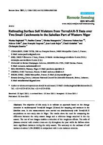
images was calculated as the TCT for the Landsat 8 OLI imagery. The approach described below was designed to accomplish the derivation of the transformation. Firstly, a total of 5404 random pseudo-invariant samples, including deep water, dense vegetation and manmade surface, were evenly selected by visual interpolation from the first nine pairs of Landsat OLI/ETM+ scenes given in Table 2 to guide the rotations. The selected objects were considered to be invariant during an 8-day interval between the paired OLI and these ETM+ images [25]. An Ordinary Procrustes analysis was then performed on all these nine pairs of Landsat scenes to align the Landsat 8 OLI principal component analysis (PCA) transformed space represented by the selected samples with the pair-wise linked Landsat 7 ETM+ tasseled cap space. The nine initial rotation matrices were subsequently defined through multiplication between the transformation coefficients developed by Procrustes and PCA. Secondly, a Generalized Procrustes analysis was adopted to obtain the consensus orthogonal rotation matrices from the nine input initial rotation matrices. The transformation was derived through a calculation of the ensemble average rotation matrix of all scenes. Finally, the Gram–Schmidt procedure was used to preserve the orthogonality of all seven axes, enabling the identification of a new set of orthogonal axes that highlighted the tasseled cap features the most for Landsat 8. A detailed description of the Procrustes analysis algorithms is provided in Supplementary Material 1. 2.5.2. Methods for Extracting the Spatial Distribution of Winter Flooded Paddies Miscellaneous rice cropping systems in the three representative provinces may pose challenges to the accurate acquisition of the soil moisture. To overcome this problem, an integrated approach was used to sense different fractional vegetation cover and soil moisture conditions from different rice cropping systems (Figure 4). With pairs of feature values (TCTW and TVDI) derived from the Landsat images and θ v measurements were obtained, the TCTW and TVDI indices were introduced as the regressors with θ v as the output in an advanced machine learning algorithm, the general regression neural network have Remote Sens.(GRNN) 2016, 8, 38 [38,39]. Over the past decade, probabilistic neural networks like GRNN 8 of 19 been widely used for solving nonlinear problems and preforming predictions because of their flexible ofstructures, their flexiblehigh network structures, highand faultrobustness tolerances, and robustness [39–46]. Additionally, the benefit network fault tolerances, [39–46]. Additionally, the primary primary benefit of GRNN over a traditional back propagation neural network is its ability to obtain of GRNN over a traditional back propagation neural network is its ability to obtain a satisfying fit a satisfying fit of the data rapidly, with only a few training samples available, and without of the data rapidly, with only a few training samples available, and without additional parameter additional parameter inputs [39,44]. These features make GRNN a very efficient tool for inputs [39,44]. These features make GRNN a very efficient tool for constructing predictors for the constructing predictors for the desired variables. desired variables.

FigureFigure 4. Flowchart of the algorithm for extracting WFP from Landsat images. 4. Flowchart of the algorithm for extracting WFP from Landsat images. After attaining the monthly paddy θv images during a winter season (December to February), a threshold was needed to differentiate the flooded paddies from non-flooded paddies in each time series of θv images. The overlapping areas of flooded rice paddies of all three tiles could then be regarded as continuously flooded paddies in winter (Figure 4). To this end, the derived SMC distribution data of paddy soil within the case study area were taken as the threshold for


8 of 18

After attaining the monthly paddy θ v images during a winter season (December to February), a threshold was needed to differentiate the flooded paddies from non-flooded paddies in each time series of θ v images. The overlapping areas of flooded rice paddies of all three tiles could then be regarded as continuously flooded paddies in winter (Figure 4). To this end, the derived SMC distribution data of paddy soil within the case study area were taken as the threshold for identifying flooded paddies. If the pixel value in the θ v image is larger than the pixel value in the according SMC image, it will then be classified as a flooded pixel. 3. Results and Discussion 3.1. Tasseled Cap Transformation Coefficients The Landsat 8 tasseled cap coefficients are listed in Table 4 and compared with the coefficients derived by Baig et al. [21]. Except for the deep blue band, the two sets of TCT coefficients are generally similar. There are, however, still some notable differences between them, and the addition of the OLI deep blue visible band may be the cause. The distribution of band weights were somewhat altered due to the added band. On the other hand, the modified methodology is another potential impact factor contributing to the differences between the two sets of coefficients. The quasi-synchronous ETM+ tasseled cap space was taken as the reference target instead of the TM transformed OLI data. These differences highlight the importance of a standardized rotation procedure of the tasseled cap transformation. Table 4. TCT coefficients for Landsat 8 OLI at-satellite reflectance. Index

Coastal Aerosol

Blue

Green

Red

NIR

SWIR1

SWIR2

Baig et al.

Brightness Greenness Wetness

/

0.3029 ´0.2941 0.1511

0.2786 ´0.2430 0.1973

0.4733 ´0.5424 0.3283

0.5599 0.7276 0.3407

0.5080 0.0713 ´0.7117

0.1872 ´0.1608 ´0.4559

This study


0.2540 ´0.2578 0.1877

0.3037 ´0.3064 0.2097

0.3608 ´0.3300 0.2038

0.3564 ´0.4325 0.1017

0.7084 0.6860 0.0685

0.2358 ´0.0383 ´0.7460

0.1691 ´0.2674 ´0.5548

Note: The Coastal aerosol band is a newly added band in Landsat 8 OLI sensor used for coastal and aerosol studies.

3.2. Confirmation of Tasseled Cap Features To confirm the tasseled cap features after transformation, nearly 7000 pseudo-invariant samples, including deep water, dense vegetation, sparse vegetation, manmade objects, and bare soil were selected randomly from the validation image (#10 image given in Table 2). The brightness, greenness and wetness axes are presented by the “tasseled cap” concept for the two transformations (Figure 5). The shapes of the selected samples from the validation scene in the two sets of tasseled cap spaces are similar, whereas their orientation and relative location differ moderately from each other (Figure 5). The greenness and wetness values of our transformation (hereafter referred to as ETM+-based TCT) were generally lower than those of Baig et al. [21] (hereafter referred to as TM-based TCT). In the brightness-greenness space, the greenness values of bare soil samples derived from the TM-based TCT are all greater than 0, and remain stable as the brightness value increases (Figure 5a). On the contrary, the ETM+-based TC transformed space reveals that the greenness values of bare soil samples are all less than 0, and there is a slight decline in its greenness value as the brightness value rises (Figure 5b). Considering that soil has the highest spectral reflectance in the short-wave infrared band (SWIR1, with a central wavelength of 1.609 µm) within the spectral range of Landsat 8 [47], a smaller loading in the SWIR1 band may lead to lower greenness values of bare soil samples obtained after transformation, making it easier to discriminate bare soil pixels from sparse vegetation pixels using the greenness alone (Figure 5). Larger disparities are found


9 of 18

in brightness–wetness/wetness–greenness space. Besides deep water, the wetness value of dense vegetation as well as a few sparse vegetation and manmade objects samples derived from TM-based TCT are also greater than 0, which shows it is not possible to distinguish water pixels from dense vegetation pixels effectively by using wetness index only. It is suggested that the ETM+-based TC transformed space could better highlight the discrepancy between water bodies and other land cover types due to the wetness values of all land cover types derived from ETM+-based TCT being negative, except water pixels, and the wetness values increasing as the brightness values generally decrease. Taken together, the vegetation cover could be identified from the land surface using a threshold of Greenness index > 0, while the water body could be easily extracted from a TCTW image using a threshold of TCTW > 0. Therefore, it would be very efficient if the TCT-derived indices were introduced Remote Sens. 2016, 8, 38 10 of 19 in a classification process.

Figure 5. Comparison of tasseled cap spaces derived by (a) Baig et al. (2014) and (b) this study.

Figure 5. Comparison of tasseled cap spaces derived by (a) Baig et al. (2014) and (b) this study. 3.3. Validation of Tasseled Cap Transformation A total of 2667 pseudo-invariant samples, including dense vegetation, deep water and manmade surfaces, were selected randomly as an independent validation dataset. Mean bias error (MBE), mean absolute error (MAE), and root-mean-square error (RMSE) were used to assess the goodness of fit between the OLI-based TC value and the quasi real-time ETM+-based TC value from the two transformations.


10 of 18

3.3. Validation of Tasseled Cap Transformation A total of 2667 pseudo-invariant samples, including dense vegetation, deep water and manmade surfaces, were selected randomly as an independent validation dataset. Mean bias error (MBE), mean absolute error (MAE), and root-mean-square error (RMSE) were used to assess the goodness of fit between the OLI-based TC value and the quasi real-time ETM+-based TC value from the two transformations. 1 ÿn (2) MBE “ i“1 pEi ´ Oi q n 1 ÿn MAE “ (3) i“1 |Ei ´ Oi | n c 1 ÿn 2 RMSE “ (4) i“1 pEi ´ Oi q n where n is the number of provinces, and Ei and Oi are the estimated and observed θ v , respectively. The MBE corresponds to the metrics of overestimation (´) and underestimation (+) [48]. The method is perfect when MBE = 0, MAE = 0 and RMSE = 0. The results achieved in terms of the three TC features are summarized in Table 5. There appeared to be an obvious overestimation of the TM-based TCT greenness (MBE = 0.0588) and wetness values (MBE = 0.0739), though the correlation coefficients of both approaches were significant at the 0.01 level. Although the estimations of brightness from the two methods were comparable, better performance for greenness and wetness was achieved by our method; the R2 increased by 0.0133 and 0.4428, the MAE decreased by 0.0312 and 0.0643, and the RMSE decreased by 0.0414 and 0.0811, respectively. Overall, it can be seen that the transform coefficients of this study can better maintain the tasseled cap features. The estimation accuracy, for the wetness index in particular, improved greatly. There are several possible explanations for the improvement in our estimation. First, there is continuity between the band settings of Landsat 8 and Landsat 7, as well as some new spectral characteristics including the addition of a deep blue band, a shortwave-infrared band, and refinement of the spectral range of several bands corresponding to those of Landsat 7 ETM+ [49]. These may bring estimation error if the TM TCT coefficients are directly applied to OLI data for creating the target feature space. Second, the DN-based TM TCT coefficients are suitable for raw DN images rather than radiometrically calibrated data. Therefore, an increase in the estimation error is likely when taking the at-satellite OLI images as input data. In addition, many studies have proven the effectiveness of at-satellite reflectance–based TCT coefficients [25,26]; however, the impacts of atmospheric scattering and sun illumination geometry still exist. The direct application of all samples to the images used to calculate the tasseled cap transformation coefficients may also lower the estimation accuracy. Our method has the capability to overcome the deficiencies mentioned above and can thereby obtain relatively accurate tasseled cap transformation indices. Table 5. Assessment of the two tasseled cap transformations. TCT

Index

R2

MBE

MAE

RMSE

Baig et al.


0.9737 0.9807 0.5454

0.0132 0.0588 0.0739

0.0338 0.0588 0.0743

0.0432 0.0719 0.0947

This study


0.9866 0.9940 0.9881

0.0432 ´0.0093 0.0010

0.0468 0.0276 0.0100

0.0567 0.0305 0.0136

3.4. Soil Moisture Content Retrieval The relationship between the TCTW, TVDI and θ v could be complicated by the presence of various vegetated conditions in rice paddies during winter [50]. The rice paddy may be partially or fully covered by rice straw, grass, or crop canopy (e.g., rape). This may have a negative effect on the θ v


11 of 18

retrieval algorithm. It has been reported that the Normalized Difference Tillage Index (NDTI) is a good indicator for differentiating vegetation/crop residue from soil [51,52]. NDTI can be calculated by surface reflectance values from the two shortwave-infrared (SWIR) bands: Remote Sens. 2016, 8, 38

NDTI “

ρSW IR1 ´ ρSW IR2 ρSW IR1 ` ρSW IR2

12 of 19

(5)

− 𝜌𝑆𝑊𝐼𝑅2values from Band 5 and Band 7 in the where ρSW IR1 and ρSW IR2 refer to the surface𝜌𝑆𝑊𝐼𝑅1 reflectance NDTI = (5) 𝜌𝑆𝑊𝐼𝑅1 + 𝜌𝑆𝑊𝐼𝑅2 OLI sensor, respectively. Therefore, as Landsat-7 ETM+ sensor and Band 6 and Band 7 in the Landsat-8 summarized fromand all the NDTI the in situ field samples, error statistics where ρSWIR1 ρSWIR2 refervalues to theatsurface reflectance values the from Band 5 and were Band calculated 7 in the for Landsat-7 ETM+ andě0.2. Band NDTI 6 and Band in the Landsat-8 OLIfractional sensor, respectively. Therefore, two NDTI classes of sensor