Jun 28, 2017 - ARC Centre of Excellence for Coral Reef Studies, James Cook University, ... of management actions aimed at its mitigation (Bryan 1971; Warwick & ...... Martin TG, Wintle BA, Rhodes JR, Kuhnert PM, Field SA, Low-Choy SJ, ...
bioRxiv preprint first posted online Jun. 28, 2017; doi: http://dx.doi.org/10.1101/157297. The copyright holder for this preprint (which was not peer-reviewed) is the author/funder. It is made available under a CC-BY 4.0 International license.
ESTIMATING THE FOOTPRINT OF POLLUTION ON CORAL REEFS USING MODELS OF SPECIES TURN-OVER
Estimating the footprint of pollution on coral reefs using models of species turn-over Christopher J. Brown Richard Hamilton 2,3
1
1. Australian Rivers Institute, Griffith University, 170 Kessels Road, Nathan, Queensland, 4111, Australia 2. The Nature Conservancy, Asia Pacific Resource Centre, 48 Montague Road, South Brisbane, QLD 4101, Australia 3. ARC Centre of Excellence for Coral Reef Studies, James Cook University, Townsville, QLD 4811, Australia
Abstract Ecological communities typically change along gradients of human impact, though it is difficult to estimate the footprint of impacts for diffuse threats like pollution. Here we develop a joint model of benthic habitats on lagoonal coral reefs and use it to infer change in benthic composition along a gradient of distance from logging operations. The model estimates both changes in abundances of benthic groups and their compositional turn-over, a type of beta-diversity. We detect compositional turnover across the gradient and use the model to predict the footprint of turbidity impacts from logging. We then apply the model to predict impacts of recent logging activities, finding recent impacts to be small, because recent logging has occurred far from lagoonal reefs. Our model can be used more generally to estimate the footprint of human impacts on ecosystems and evaluate the benefits of conservation actions for ecosystems.
Introduction Determining the extent and impact of diffuse threats, like pollution, is an important concern for ecological science and management. For instance, the extent of pollution impacts on marine benthic communities is often used to estimate the benefits of management actions aimed at its mitigation (Bryan 1971; Warwick & Clarke 1991; De’ath & Fabricius 2010; DeMartini et al. 2013). Evaluating the ecological benefits of mitigative efforts requires spatially comprehensive mapping of the ecosystems that are significantly affected. When the impact of a threat on different species varies, changes in community composition can be used to infer the spatial extent of a diffuse threat (Warwick 1993). For instance, coastal development can increase turbidity of waters, causing shifts in coral reef communities toward stress tolerant species (e.g. Guest et al. 2016). Thus, species turnover, or beta-diversity, can be used to determine how far along a gradient one must move before the community is significantly changed (Anderson et al. 2011; Socolar et al. 2016). The spatial extent of diffuse impacts to communities can be challenging to infer from patchy measurements. Here we refer to ‘community composition’ as any multivariate measure of the abundance of organisms that make-up a community, including both species and higher taxonomic groupings. We will also refer to measurements made on counts of individuals, occurrences of a taxonomic group or per cent cover collectively as ‘abundances’. The analysis of community change over physical gradients presents many technical challenges. In particular, there are often many species sampled across relatively few sites. Algorithms for the analysis of multivariate abundances help overcome this problem (e.g. Kruskal 1964; Anderson et al. 2011; Legendre & Legendre 2012). However, current methods are limited in that they are typically not based on models of abundances so, while they can be used to test for significant differences in community composition, they cannot predict abundances to unsampled sites (Warton et al. 2015). Prediction at unsampled sites is crucial for estimating the extent of a diffuse threat when measurements are patchy. Multivariate statistical models of abundances can directly model the effects of environmental covariates and thus enable prediction of community composition at unsampled sites (Warton et al. 2015). These new methods, termed ‘joint modelling’ build on generalised linear models to allow inclusion of multiple species and their interactions with each other and environmental covariates (Hui et al. 2015; Warton et al. 2015). Joint Brown and Hamilton. Pre-print
1
bioRxiv preprint first posted online Jun. 28, 2017; doi: http://dx.doi.org/10.1101/157297. The copyright holder for this preprint (which was not peer-reviewed) is the author/funder. It is made available under a CC-BY 4.0 International license.
ESTIMATING THE FOOTPRINT OF POLLUTION ON CORAL REEFS USING MODELS OF SPECIES Methods TURN-OVER
models can also be used to estimate uncertainty in species-environment relationships. Abundance models may commonly have increased power to detect change in abundances when compared to traditional ordination methods, making them useful for detecting the response of rare species to human disturbances. However, joint models are a relatively recent development (Warton et al. 2015), so their application to conservation issues has been limited to date. Here we sought to develop a new type of joint model that could estimate the areal footprint of diffuse threats, like pollution, on ecological communities. We developed a model that builds on recent methods for Bayesian ordination (Hui et al. 2015; Hui 2016). The new development is the inclusion of constrained latent variables that represent turn-over in the composition of the benthic community across a gradient of pollution impacts. Our model is a generalisation that allows for covariates to effect the latent variables, rather than directly affecting species abundances. The model could also be viewed as a type of Bayesian structural equation model (e.g. Joseph et al. 2016), or as a Bayesian analog to constrained factor analysis. By using distance from a source of pollution as the covariate the constrained latent variable can be interpreted as an unobservable gradient of community change. The rate of change in the latent variable in response to the threat represents community turn-over and so is interpretable as a measure of beta-diversity (Anderson et al. 2011). To illustrate the utility of joint modelling in conservation, we apply the model to survey data of coral reef communities in the Kia region of Solomon Islands. Around Kia sediment run-off from logging operations has degraded lagoonal reefs (Hamilton et al. 2017). We applied the joint model to surveys of lagoonal reef communities that were conducted across a gradient of distances from logging operations. We aimed to address three objectives in the case-study. First, we sought to quantify how different components of the benthic community respond to sediment run-off from logging and identify interactions among benthic habitats. We also asked whether these community responses were consistent with studies of coral reef communities from other regions. Second, we aimed to estimate the areal footprint of logging impacts on benthic communities. Finally, new illegal logging has occurred in the region since the original surveys and here we aim to estimate how much more reef has been affected by these illegal operations. More generally, our objective is to use the case-study to illustrate how joint modelling can be applied to estimate the impact of new developments, or the benefits of conservation actions.
Methods First we describe a general framework for modelling community composition as a function of latent variables and their covariates. Then we describe a specific application of the model to benthic communities in the Solomon Islands. Model framework We modelled abundances of multiple response groups as a function of multiple latent variables (Fig 1). The method built on existing models for Bayesian ordination (Hui 2016). The response groups could represent species, taxonomic groups, or as in our case-study below, habitat categories. The abundance of each group was modelled as a function of a linear predictor:
ηi,j = θi + αj +
K X
βj,k γi,k
k=1
Equation 1 Where θi was an offset term that accounted for variation in sampling intensity across sites, ηi,j was the value of the linear predictor for group j at site i, αj is a group level intercept term, which allows among group variability in average abundances across all sites. The summation is over K latent variables which take values γi,k at each site. Finally, βj,k is a group’s loading on a given latent variable. Equation 1 is flexible in that it can be used with a range of statistical distributions to model different types of observations including counts, occurrences or per cent cover data. Brown and Hamilton. Pre-print
2
bioRxiv preprint first posted online Jun. 28, 2017; doi: http://dx.doi.org/10.1101/157297. The copyright holder for this preprint (which was not peer-reviewed) is the author/funder. It is made available under a CC-BY 4.0 International license.
ESTIMATING THE FOOTPRINT OF POLLUTION ON CORAL REEFS USING MODELS OF SPECIES Methods TURN-OVER
The latent variables were sampled from normal distributions: γi,k ∼ N (κi X, 1) Equation 2 Where there are K latent variables across the i sites, κk is a vector of coefficients and X is a matrix of covariate values across the sites. Latent variables for residual correlations have κk = 0. An alternative model would be to specify direct effects of the covariates on each group’s abundance (Hui et al. 2015). The primary difference between a direct effects model and our proposed model is that our proposed model estimates only one coefficient for the spatial attenuation of the threat, whereas the direct model estimates one attenuation coefficient per group. This difference results in a subtle but important difference in interpretation of environmental effects to abundances. The coefficients for the direct model are interpretable in terms of change in abundance of individual groups with environmental change, for instance, a poisson model of abundance would estimate the rate of change in the log of abundance over environmental change. Our proposed approach loses some interpretability at the individual group level, but gains interpretability at the community level. The attenuation coefficient now represents the rate of change in an ordination of community composition across the environmental gradient. The constrained latent variable estimated in our proposed approach could be interpreted in multiple ways. If abundances are taken to be imperfect indicators of a latent environmental state, like turbidity, then the latent variable represents our best estimate for the extent of turbid waters. Taking the latent variable as a measure of turbidity also means we should interpret its coefficients (κk = 0) as representing attentuation of turbidity over space. Abundances could also be interpreted as imperfect indicators of an underlying community gradient, in which case the latent variable represents our best estimate of the community’s state with respect to the gradient. If we take the community-centric interpretation then the latent variable’s coefficient is a measure of community turn-over across the gradient (i.e. beta-diversity) (Anderson et al. 2011). To aid interpretation we transform the constrained latent variable to a 0-1 scale using the probit function. On the probit scale, values near 0 or 1 represent communities that are at extreme ends of the composition gradient. Higher estimated values of the coefficient κk for an environmental gradient X mean the probit transform will approach 0 and 1 at either end of the gradient. If κk is near zero then community composition does not vary across the gradient and all values on the probit scale will be near 0.5. Priors for species loadings (βj,k ) and covariate effects (κk = 0) are specified using normal distributions. We use uninformative priors for covariate effects (mean = 0, variance = 1000) and vaguely informative priors for species loadings (mean = 0, variance = 20) to aid convergence (Hui 2016). Vaguely informative priors are appropriate here because we standardised data, so we do not expect variances or effects to be >> 1.
Brown and Hamilton. Pre-print
3
bioRxiv preprint first posted online Jun. 28, 2017; doi: http://dx.doi.org/10.1101/157297. The copyright holder for this preprint (which was not peer-reviewed) is the author/funder. It is made available under a CC-BY 4.0 International license.
ESTIMATING THE FOOTPRINT OF POLLUTION ON CORAL REEFS USING MODELS OF SPECIES Methods TURN-OVER
Figure 1 Directed graph giving an example for the structure of our Bayesian latent variable model applied to coral reef habitats in Solomon Islands. Squares indicate measured variables, circles indicate latent variables, variables in italics also have error terms that are estimated from the data. Arrows indicate model effects, with gray and black arrows indicating the effects relating to different latent variables. Case-study We model change in cover of benthic habitats across a gradient of sedimentation in the Kia District of Isabel Province, Solomon Islands. Logging in Kia district has removed 50% of forests over the last 15 years. Typical operations haul logs to log ponds, which are locations on the coast where mangroves are bulldozed so logs can be stored then transported elsewhere. Log ponds result in significant sedimentation entering nearshore environments, which smothers corals and causes declines in branching corals and fish that depend on those corals for habitat (Hamilton et al. 2017). The southern part of the district has extensive logging (Hamilton et al. 2017), whereas the northern section was unlogged when the survey data were collected in 2013.
Brown and Hamilton. Pre-print
4
bioRxiv preprint first posted online Jun. 28, 2017; doi: http://dx.doi.org/10.1101/157297. The copyright holder for this preprint (which was not peer-reviewed) is the author/funder. It is made available under a CC-BY 4.0 International license.
ESTIMATING THE FOOTPRINT OF POLLUTION ON CORAL REEFS USING MODELS OF SPECIES Methods TURN-OVER
Previously the region-wide loss of nursery habitat was estimated based solely on the area of reefs within each region (Hamilton et al. 2017). Here we seek more accurate estimates for the extent of degradation of reef habitats and also to investigate relationships among different habitat types and sediment. Additionally, some illegal logging has occurred in the north-western part of the region, which before 2013 was unlogged. The recent illegal logging may have affected the relatively pristine northern reefs, which are important habitat for bumphead parrotfish (Bolbometopon muricatum), a locally important fishery species that is also listed as threatened on the IUCN Red List (Hamilton et al. 2017). Thus a second objective of this study was to estimate the area of lagoonal reefs that may have been affected by this illegal logging. The data include surveys of benthic communities at 49 sites, conducted in October 2013 (Hamilton et al. 2017). Sites were surveyed using a modified version of the point intercept method (Hill & Wilkinson 2004). Benthic habitats were recorded every 2 m along a 50 m transect, taking three measurements at each point, which were located directly below and one metre to the left and right of the transect. There were five transects of 75 points at each site, making a total of 375 points per site. Benthic habitats were categorised as per English et al. (1994), however we added categories for Acropora Branching Dead and Coral Branching Dead. Water clarity was also measured in deep water near to survey sites using a Secchi disc. For analysis we aggregated categories into 17 focal groups (Appendix S1). Aggregation sped computations and emphasised change in the habitat types we were most interested in. We also aggregated categories to avoid having numerous infrequently recorded categories that had many zeros. Rare categories would require additional modifications of the model to allow for over-dispersion (e.g. zero-inflated models Martin et al. (2005)), which is beyond the scope of this initial analysis. Cover (number of points out of 375) of the benthic habitats at each site was modelled as a multinomial variate, using a mix of poisson distributions (Gelman & Hill 2006). The poisson model for the count of points belonging to each habitat was specified using a log-link as per equation 1. To ensure the model parameters are identifiable the habitat-level intercepts (αj ) are modelled as a random effect (Gelman & Hill 2006). Predictions for proportional cover of each habitat at each site can then be obtained by normalising predictions for the count of each habitat by the sum of expected counts across all habitats: eπi,j pi,j = PJ πi,j j=1 e Equation 3 Where πi,j is the expectation for the count of habitat j at site i, αj is a habitat-specific random effect, βj . We addressed the first objective, which was to quantify community responses to logging, by performing model selection to identify and best model and then visualising mean responses to log ponds (with 95% credibility intervals) for the entire community and each component habitat. The first latent variable was modelled as a function of distance to the nearest log pond and flow strength. We standardised the distance metric by subtracting its mean dividing by its standard deviation. Flow was classified as either low or high, based on experience of the survey divers. Previous analysis indicated that flow strength was important for explaining cover of branching corals (Hamilton et al. 2017). For all covariates we estimated mean effects with 95% credibility intervals, where a 95% CI that does not overlap zero is statistically significant. As an additional test of the model we compared the estimates of the sedimentation latent variable to Secchi depths that were measured during surveys (Hamilton et al. 2017). We also included two unconstrained latent variables in the model to account for residual correlations among habitat categories. We decided to use two latent variables, because results from two latent variables can be easily visualsed (Hui 2016). In additional simulations we refit the models with up to 4 unconstrained latent variables. We also fit a model with two unconstrained latent variables and no constrained latent variables and compared its fit to the model with a constrained latent variable using the Watanabe-Akaike information criterion (WAIC) (Vehtari et al. 2016) We checked model fits by comparing predicted to observed per cent covers for each habitat type and also checked counts of points using rootograms (Kleiber & Zeileis 2016). We calculated the bias and variance in
Brown and Hamilton. Pre-print
5
bioRxiv preprint first posted online Jun. 28, 2017; doi: http://dx.doi.org/10.1101/157297. The copyright holder for this preprint (which was not peer-reviewed) is the author/funder. It is made available under a CC-BY 4.0 International license.
ESTIMATING THE FOOTPRINT OF POLLUTION ON CORAL REEFS USING MODELS OF SPECIES Results TURN-OVER
predicted to observed cover levels. We addressed our second objective of mapping the footprint of logging by predicting the constrained latent variable across the entire study region, using as a covariate the over water distance to the nearest log pond. Because we did not have flow estimates for the entire study region, we assumed low flow at all sites, which was the dominant condition at surveyed reefs. We then applied the probit link function to map the values of the latent variable onto a 0-1 probability scale. Finally, we estimated the area of reefs within probability bands of 95%, 75%, 50% and 25%, where higher values indicate community composition closer to log-ponds. For reefs that were outside the range of distances from log ponds observed in the surveys we used the minimum and maximum observed distances to predict the condition variable, which avoided extrapolation. Our final objective was to estimate the area of lagoonal reefs affected by new logging operations. We repeated the calculations for the area of reef affected by logging with new logging that has recently occurred logging on the north-western Coast (three log ponds at: [7.43639oS , 158.19973oE ], [7.42830oS , 158.20321oE ] and [7.42558oS , 158.20111oE ]) and then we calculated the area of reefs that are predicted to be affected by increased turbidity. We used JAGS (Plummer & others 2003) for parameter estimation, run from the R programming environment (R Core Team 2016) using the package rjags (Plummer 2016). For each model we ran a single chain with 1 000 000 samples, thinning for every 40th sample. We used only a single chain to avoid issues with parameter switching on the latent variables (Hui 2016). We checked the Hellinger distance statistic (Boone et al. 2014) to confirm model convergence. Data are provided in Appendices S1-3, JAGS model code is provided in Appendix S4.
Results The model with a constrained latent variable and two unconstrained variables had stronger support than the ordination that had no constrained latent variables (Table 1). Adding more unconstrained variables also increased the support for the model (Table 1), but simultaneously weakened the effect of the constrained latent variable (Appendix S5). However, we proceed with analysis using the model that had two unconstrained and one constrained latent variables. Table 1 Model comparison using the WAIC. LV: number of unconstrained latent variables. Model
WAIC
Bayesian ordination, 2 LVs Constrained model, 1 LV Constrained model, 2 LV Constrained model, 3 LV Constrained model, 4 LV
15621 15679 12123 10093 8243
There was a significant positive effect of minimum distance to log ponds on the constrained latent variable (median = 0.47, 0.12 to 0.81 95% C.I.s), that was in the same direction as high flow conditions (median = 1.91, 0.9 to 2.93 95% C.I.s). The median effect of high flow was ~4 times greater than the median effect of minimum distance on the latent variable. Thus, we can interpret a change from low to high flow as having an equivalent effect on community structure as moving 2.46 km further away from log-ponds. We checked the nearest distance model for bias in its predictions of each habitat separately (Appendix S5). In general the model fitted most habitats with low bias. Bias was higher for habitats that had many zero observations, where the model tended to underpredict their counts in surveys. The loadings of the habitats on the constrained latent variable indicated that it represents a gradient from high cover of branching Acropora, branching corals, dead branching corals, other habitats and rare corals far from log-ponds, towards higher cover of soft sediment, Halimeda algae, dead corals, macro-algae, turf algae and massive corals closer to log-ponds (figs 2a, 4). At sites far from log ponds, branching Acropora were Brown and Hamilton. Pre-print
6
bioRxiv preprint first posted online Jun. 28, 2017; doi: http://dx.doi.org/10.1101/157297. The copyright holder for this preprint (which was not peer-reviewed) is the author/funder. It is made available under a CC-BY 4.0 International license.
ESTIMATING THE FOOTPRINT OF POLLUTION ON CORAL REEFS USING MODELS OF SPECIES Results TURN-OVER
commonly observed growing out of sand, so the high cover of soft sediments but low cover of Acropora at sites near to log ponds ostensibly indicates the loss of Acropora. Multiple algae groups were als associated with sites closer to log ponds (Fig 3a), however their overall change increase closer to log ponds was small (Fig 3), suggesting they maintained their cover across the gradient, rather than replacing other habitats. Overall, cover of algae was low (