Keywords: Big Data, parameter estimation, model updating, system. identiï¬cation ... Ï(θ) is deï¬ned as a target probability distribution, from which one wishes to.
Estimating the parameters of dynamical systems from Big Data using Sequential Monte Carlo samplers P.L.Greena,c , S.Maskellb,c a School of Engineering Department of Electrical Engineering and Electronics c Institute for Risk and Uncertainty University of Liverpool Liverpool, UK L69 7ZF
rin t
b
Abstract
ep
In this paper the authors present a method which facilitates computationally efficient parameter estimation of dynamical systems from a continuously growing set of measurement data. It is shown that the proposed method, which utilises Sequential Monte Carlo samplers, is guaranteed to be fully parallelisable (in contrast to Markov chain Monte Carlo methods) and can be applied to a wide variety of scenarios within structural dynamics. Its ability to allow convergence of one’s parameter estimates, as more data is analysed, sets it apart from other sequential methods (such as the particle filter).
Pr
Keywords: Big Data, parameter estimation, model updating, system identification, Sequential Monte Carlo sampler.
1. Introduction
This paper addresses the situation where one is attempting to infer the parameters of a dynamical model from a large set of data which, because of its size, cannot be processed using current methods. Here, z t denotes a vector of measurements, obtained at time t, and θ is a vector of the model’s parameters. The aim is to realise probabilistic estimates of θ, given the available data, via Bayes’ theorem: p(θ | z 1:n ) ∝ p(z 1:n | θ)p(θ)
(1)
where z 1:n = {z 1 , ..., z n } represents the set of all measurements up to time t = n. In [1, 2] it was suggested that, using Markov chain Monte Carlo (MCMC) methods, one could generate samples from p(θ | z 1:t ) while t is gradually increased. Such an approach facilitates a gradual transition from prior to posterior, which aids MCMC convergence (in a similar manner to
rin t
simulated annealing). It also allows one to analyse how one’s parameter estimates converge as more data is analysed, thus helping to establish when a sufficient amount of data has been utilised. The computational cost of such an approach, however, increases dramatically as more data is analysed. This makes it poorly suited to the situation where large sets of new (potentially important) measurements are expected to arrive in the future. Other approaches such as [3] involve the selection of small subsets of ‘highly informative’ training data from large data sets. While this reduces computational cost, it involves the deliberate omission of measurement data which, in hindsight, may contain important information (and reduce uncertainty in the posterior as a result).
ep
In this paper, an algorithm based on Sequential Monte Carlo (SMC) methods is proposed, which is able to address the aforementioned issues. Fundamentally, the efficiency of the method proposed here lies in its ability to exploit the inevitable redundancies that arise in large sets of measurements, as well as its suitability for modern computing architectures. In the interest of completeness, a brief introduction to SMC methods, as well as a description of previous work relevant to the problem of interest, is given in the following section.
2. Sequential Monte Carlo methods 2.1. Importance sampling
Pr
This section begins with a brief description of importance sampling. Here π(θ) is defined as a target probability distribution, from which one wishes to estimate the expected value of a function, f (θ). π ∗ (θ) is used to represent an unnormalised target, such that: Z π ∗ (θ) π(θ) = , Z = π ∗ (θ)d θ (2) Z (for generality it is assumed that Z is difficult to estimate here - a situation which often arises in Bayesian inference problems). The expected value of f (θ) can be written as R R f (θ)π ∗ (θ)d θ f (θ)q(θ)w(θ)d θ R E[f (θ)] = = R (3) ∗ π (θ)d θ q(θ)w(θ)d θ ∗
(θ) where w(θ) = πq(θ) are ‘importance weights’ and q(θ) is a user-defined ‘proposal distribution’ - a probability distribution from which it is relatively easy to generate samples. Equation (3) implies that
2
E[f (θ)] ≈
N X
f (θ i )w ˜i
(4)
i=1 1
N
where {θ , ..., θ } have been generated from q(θ) and, adopting the notation wi ≡ w(θ i ), wi w ˜i = P j , jw
i = 1, ..., N
(5)
rin t
are defined as ‘normalised importance weights’. This reweighting procedure allows estimates of E[f (θ)] to be realised using samples from q(θ), which is useful when it is difficult to generate samples from the target distribution, π(θ), directly. 2.2. Resampling
By defining f (θ j ) = δ(θ j − θ) where δ is the Dirac delta function, it follows that Z E[f (θ j )] = δ(θ j − θ)π(θ)d θ = π(θ j ). (6)
ep
This implies that, if one has a set of samples (and accompanying normalised ¯ 1 , ..., θ ¯ N }, is weights) {θ 1 , w ˜ 1 }, ..., {θ N , w ˜ N } while a new set of samples, {θ chosen such that ¯ = θi ) = w Pr(θ ˜i
(7)
Pr
¯ 1 , ..., θ ¯ N } will be approximate samples from the target. The weights then {θ of these new samples will therefore be equal (for more information the tutorial [4] is recommended). Resampling is often used when it is found that relatively few of the current samples have significant weight, as it helps to remove those which are of little importance. It is often used to tackle the ‘degeneracy problem’ that is often encountered in the application of particle filters. To indicate when resampling is required, the concept of ‘effective sample size’ was introduced in [5, 6]. This involves defining 1 ˜ i )2 i (w
Nef f = P
(8)
and choosing to conduct resampling when Nef f falls below some kind of threshold (N/2, for example, is used throughout the current paper). It should be noted that, while resampling helps to remove ‘unimportant’ samples, it doesn’t aid exploration of the parameter space - it can only produce replicas of the existing samples.
3
rin t
2.3. Previous work As mentioned previously, one of the best-known SMC methods is the particle filter, which can be used to ‘track’ the state of a system from a continuous stream of ‘online’ measurements - this was used in [7] to monitor the time changing parameters of dynamical structures and systems. The application of a particle filter involves defining a prediction equation, which specifies how a system’s state is expected to change (conditional on its previous state). In the scenario of interest here, justifying one’s choice of prediction equation would be rather difficult. Furthermore, when applying a particle filter, the influence of the initial measurements on the parameter estimates will decrease as more data is analysed [8]. This makes particle filters poorly suited to the current application (where it is required that all available measurements, with equal weighting, are used to infer parameter estimates). A different approach was proposed in [9] where, using the prior as a proposal distribution, importance sampling was used to target the posterior parameter distribution. At time t, this leads to the following expression for the importance weights: p(z 1:t | θ)p(θ) = p(z 1:t | θ). (9) p(θ) Assuming that the probability of witnessing separate measurements is conditionally independent, such that
ep
wt =
Pr
p(z 1:t | θ) =
t Y
p(z i | θ),
(10)
i=1
equation (9) can be used to show that wt = p(z t | θ)wt−1 .
(11)
This allows the update of the importance weights to be conducted recursively, circumventing the need to repeatedly analyse the entire set of training data. Unfortunately, this method suffers from the same degeneracy problem as the particle filter where, after a time, only very few of the samples have significant weight. As stated previously, resampling can only help to generate replicas of these samples, and does not aid a further exploration of the parameter space. In [9] this was overcome with an ‘move step’ which was facilitated using MCMC updates. This process, which involves analysis of the entire data set up to time t, was repeated every time a new measurement was obtained and, as a result, is computationally expensive to implement. In this paper it is shown that this issue can be tackled efficiently and simply using a Sequential Monte Carlo sampler. At this point it is important 4
to note that, somewhat confusingly, SMC samplers are a specific member of the family of SMC methods (to which particle filters also belong). A general description of SMC samplers is given in the following section. A more detailed theoretical explanation can be found in [10] while a description written within the applied context of automated navigation is given in [11].
3. Sequential Monte Carlo samplers 3.1. General formulation
rin t
Here, θ k is used to represent the state of a system at iteration k, πk (θ k ) is defined as the kth target distribution and π(θ 1:k ) represents the joint distribution over θ 1:k . One begins by defining π(θ 1:k ) = πk (θ k )
k Y
L(θ k0 −1 | θ k0 )
(12)
k0 =2
ep
where L(θ k0 −1 | θ k0 ) - the ‘L-kernel’ - is a design parameter which is defined such that Z π(θ 1:k )d θ 1:k−1 = πk (θ k ) (13) R R (thus realising the property that f (θ k )π(θ 1:k )d θ 1:k = f (θ k )πk (θ k )d θ k ). Potential choices for the L-kernel are described subsequently. With proposal distribution q(θ 1:k ), the importance weights are defined as π(θ i1:k ) , q(θ i1:k )
Pr wki =
θ i1:k ∼ q(θ 1:k ).
(14)
Choosing a proposal of the form q(θ 1:k ) = q(θ k | θ k−1 )q(θ 1:k−1 ) then allows one to write wki
=
Qk
i i k0 =2 L(θ k0 −1 | θ k0 ) . q(θ ik | θ ik−1 )q(θ i1:k−1 )
πk (θ ik )
(15)
i Dividing wki by wk−1 , it is then possible to show that i wki = wk−1
πk (θ ik ) L(θ ik−1 | θ ik ) πk−1 (θ ik−1 ) q(θ ik | θ ik−1 )
(16)
such that the importance weights can be sequentially updated as k increases. At first glance one may consider replacing the index k with the index t and applying the SMC sampler directly to the problem described in Section 1, such that
5
πt (θ t ) ≡ p(θ | z 1:t ).
(17)
This will, however, involve analysis of the full data set every time new measurements are analysed. The computational cost of this would make such an approach impractical. It should be noted that, in the current work, SMC samplers are actually used to facilitate the resampling step of the method proposed in [9] (hence the disparity between the indexes k and t). Before this process can be described fully, it is worth stating how SMC samplers can be used to sample from a stationary target - one which doesn’t vary with the index k.
rin t
3.2. Sampling from an invariant target
Consider the situation where one wishes to estimate the mean of an (unnormalised) target distribution π ∗ (θ). Here, the index k is simply used to denote the kth estimate of the mean. Having defined the proposal distributions q(θ 1 ) and q(θ k | θ k−1 ), algorithm 1 shows how this can be achieved using a SMC sampler.
ep
Algorithm 1 Targeting a stationary distribution using a SMC sampler. k=1 Sample {θ 1k , ..., θ N k } from q(θ k ) π ∗ (θ i )
Initial weights: wki = q(θik) , i = 1, ..., N k while do wi Normalise weights: w ˜i = P k j , i = 1, ..., N j
wk
Pr
Estimate quantities of interest Nef f = P (1w˜i )2 i if Nef f < N/2 then Resample to get {θ 1k , ..., θ N k } Reset weights: wki = 1, i = 1, ..., N end if k =k+1 i Sample {θ 1k , ..., θ N k } from q(θ k | θ k−1 ) π ∗ (θ i ) L(θ ik−1 | θ ik ) , i i k−1 ) q(θ k | θ k−1 )
i k New weights: wki = wk−1 π ∗ (θ i
i = 1, ..., N
end while Note that choosing the L-kernel L(θ k−1 | θ k ) = q(θ k−1 | θ k ) allows the weights to be updated according to
6
(18)
i wki = wk−1
π ∗ (θ ik ) . π ∗ (θ ik−1 )
(19)
As an example, a SMC sampler will be used to estimate the mean of the target distribution π(θ) = N (θ; µ, σ 2 )
(20)
where µ = 5 and σ = 0.5. For this example the proposal distributions and L-kernel are defined as: q(θk |θk−1 ) = N (θk ; θk−1 , 1),
rin t
q(θ1 ) = N (θ1 ; 0, 1),
L(θk−1 |θk ) = N (θk−1 ; θk , 1).
(21)
Using 100 samples, the resulting estimate of the mean, as a function of k, is shown in Figure 1. 5.5
4 3.5 3
ep
4.5
Pr
Estimated mean
5
2.5
2
0
20
40
60
80
100
k
Figure 1: Estimating the mean of a stationary distribution using a SMC sampler.
In the formulation shown in algorithm 1, all previous samples of θ are ‘saved’ as k increases. In the following applications this isn’t necessary algorithm 2 therefore shows an alternative form of algorithm 1, where this notation has been dropped (this also establishes a clearer notation for the algorithms described later in the paper).
7
Algorithm 2 Targeting a stationary distribution using a SMC sampler (without the index k). Sample {θ 1 , ..., θ N } from q(θ 1 ) ∗ i Initial weights: wi = πq(θ(θi )) , i = 1, ..., N while do i Normalise weights: w ˜ i = Pw wj , i = 1, ..., N j
∗
rin t
Estimate quantities of interest Nef f = P (1w˜i )2 i if Nef f < N/2 then Resample to get {θ 1 , ..., θ N } Reset weights: wi = 1, i = 1, ..., N end if ˆ θi ) Sample {θˆ1 , ..., θˆN } from q(θ| ˆi
i
ˆi
(θ ) L(θ |θ ) New weights: w ˆ i = wi ππ∗ (θ , i ) ˆi i q(θ | θ )
ˆi, Set wi = w ˆi , θi = θ end while
i = 1, ..., N
i = 1, ..., N
ep
4. Parameter estimation of static models
In this section it will be shown how, by using a SMC sampler to facilitate resampling, it is possible to conduct the sequential parameter estimation of static models from large sets of data. (Here the phrase ‘static models’ is used to distinguish the current example from the dynamical, autoregressive models investigated later in the paper).
Pr
4.1. Algorithm Consider a model of the form
y t = f (xt , θ)
(22)
where xt represents an input to the system (at time t) and, as before, θ is a vector of the model’s parameters. It is assumed that measurements are realised according to � ∼ N (�; 0, Σ� )
z t = h(y t ) + �,
(23)
(such that � represents measurement noise) where the covariance matrix, Σ� , is assumed to be known. Finally, it is also assumed that the probability of witnessing sequential measurements are conditionally independent (as in equation (10)). Algorithm 3 shows how, using the proposed method, sequential estimates of the model’s parameters can be realised. The method proceeds in a similar way to that proposed in [9], until the effective sample size drops below a predefined threshold. When this occurs, resampling is 8
used to remove those samples with low weights, before a SMC sampler is used to facilitate ‘movement’ - to explore the parameter space. It is important to note that the SMC sampler must be allowed to run until the effective sample size has recovered and that the quantities of interest are always estimated after the SMC sampler has run (this prevents them from being based on samples with a low effective sample size). While the SMC sampling step will involve a ‘full analysis’ of all the existing data, algorithm 3 has the following useful properties:
rin t
1. The SMC sampler will only be used if the effective sample size drops below a predefined threshold. 2. The SMC sampler is well suited to parallel processing, thus allowing the full exploitation of modern computing architectures. Algorithm 3 Sequential parameter estimation of a static model using the proposed methodology.
ep
Sample {θ 1 , ..., θ N } from p(θ) Initial weights: w1i = p(z 1 | θ i ), i = 1, ..., N t=1 while do wi Normalise weights: w ˜i = P t j , i = 1, ..., N j
wt
P 1 i 2 ˜ ) i (w
Pr
Nef f = while Nef f < N/2 do Resample to get {θ 1 , ..., θ N } i = 1, ..., N Reset weights: wti = 1, 1 N ˆ ˆ ˆ θi ) Sample {θ , ..., θ } from q(θ| ˆi
i
ˆi
p(z 1:t |θ ) L(θ |θ ) New weights: w ˆ i = wti p(z , | θi ) ˆ i i
ˆ i and Set wti = w ˆi , θi = θ Normalise weights:
w ˜i
q(θ | θ ) i i , y1:t = yˆ1:t i w P t j j wt
1:t
=
i = 1, ..., N i = 1, ..., N
Nef f = P (1w˜i )2 i end while Estimate quantities of interest t=t+1 i p(z | θ i ) New weights: wti = wt−1 t end while
4.2. Choice of proposal density The efficiency and repeatability of any algorithm which utilises importance sampling is heavily dependent on the choice of proposal distribution. Consider, again, the situation where the aim is to estimate the quantity 9
R E[f (θ)] = f (θ)π(θ)d θ using importance sampling. Writing the resulting estimate as fˆ =
N X
f (θ i )w ˜i
(24)
i=1
(where {θ 1 , ..., θ N } have been generated from the proposal distribution q(θ)), then it is possible to show that fˆ is an unbiased estimator, such that E[fˆ] = E[f (θ)].
(25)
rin t
The variance of fˆ can also be shown to be c E[f 2 (θ)] N where c is a constant and it has been assumed that Var[fˆ] =
π(θ)