Estimation and Experimental Validation of Borehole ... - Springer Link

KSCE Journal of Civil Engineering (2014) 18(4):992-1000 Copyright ⓒ2014 Korean Society of Civil Engineers DOI 10.1007/s12205-014-0454-x

Geotechnical Engineering

pISSN 1226-7988, eISSN 1976-3808 www.springer.com/12205

TECHNICAL NOTE

Estimation and Experimental Validation of Borehole Thermal Resistance Gyu-Hyun Go*, Seung-Rae Lee**, Seok Yoon***, Hyunku Park****, and SKhan Park***** Received September 4, 2012/Revised 1st: April 16, 2013, 2nd: June 19, 2013/Accepted July 25, 2013

··································································································································································································································

Abstract This paper focuses on an evaluation of current borehole-thermal-resistance-estimation models based on a Thermal Response Test (TRT). For the TRT, a U-type heat exchanger was installed in a single medium formed in a model box, and the test performed for about 18 hours. In order to estimate the borehole thermal resistance, two imaginary circles were regarded as the borehole boundary where the two Resistance Temperature Detector (RTD) sensors were buried. The values of thermal resistance determined from the series-sum and multipole methods were compared to each other, as well as to the results from the thermal response test and numerical simulation. With reference to the experimental results, numerical analysis and multipole methods and Remund’s model predicted reasonable results. Using the multipole method and numerical simulation, it was possible to estimate the borehole thermal resistance in a composite region. It was found that the thermal conductivity of the grout had a great influence on the borehole thermal resistance. However, this effect became smaller as the grout thermal conductivity increased. Keywords: geothermal energy, borehole thermal resistance, series sum method, multipole method, thermal response test; numerical analysis ··································································································································································································································

1. Introduction As one of the most efficient and eco-friendly renewable energy resources, geothermal energy provided by a Ground-Coupled Heat Pump (GCHP) has been gaining global attention for heating and cooling buildings. GCHP systems extract thermal energy from the ground (for heating) or inject thermal energy into the ground (for cooling) using vertical or horizontal Ground Heat Exchangers (GHEs). In these systems, a forced convective heat transfer occurs between water circulating in a pipe, and the surrounding ground or grout. In general, vertical GHEs are preferred to horizontal GHEs due to their higher energy efficiency and smaller amount of land required for installation. Accordingly, a number of design methods for vertical GHEs have been proposed to calculate the heat transfer between the GHE and the ground (Geothermal Design Studio, 2007; Hellstrom and Burkhard, 2000). In general, the design methods assume that the GHEs exist as a group of lines or cylindrical heat sources with finite lengths; then, the problem of conduction in the ground is solved based on analytical or semi-analytical schemes. The mean temperature of the fluid circulating within the GHE is estimated considering a one- or two-dimensional thermal resistance network in a cross section of the GHE. If a steady heat flow is maintained around the GHE, the difference between the mean fluid temperature

and the temperature at the borehole-soil interface has a unique proportional relationship with the heat transferred. The proportional factor is generally called the borehole thermal resistance (Claesson and Hellstrom, 2011; Mostafa et al., 2009). Hence, for a reasonable GHE design, reliable estimation of ground thermal conductivity, and borehole thermal resistance, is essential. While the thermal conductivity is an inherent parameter, the borehole thermal resistance depends on various components of the GHE: convective heat transfer characteristics of the fluid, thermal properties of the pipe and the grout, number of pipes, and arrangement. Hence, various empirical, analytical, and numerical models have been proposed for the estimation of borehole thermal resistance (Bennet et al., 1987; Gu and O’Neal, 1998; Claesson and Hellstrom, 2011; Liu et al., 2009; Mostafa et al., 2009; Roth et al., 2004; Remund, 1999; Shonder and Beck, 1999; Young, 2001). In one case, an empirical model was suggested based on experimental data (Remund, 1999); however, experimental validation of the current models is still lacking. Because thermal resistance plays an important role in the design of a GCHP system, effective estimation of borehole thermal resistance is directly linked to the economic design of the GCHP system (Marcotte and Pasquier, 2008). In other words, once a reliable borehole resistance is determined, it is possible to control the amount of flux in the fluid temperature

*Graduate Student, Dept. of Civil and Environmental Engineering, KAIST, Daejeon 305-701, Korea (E-mail: [email protected]) **Member, Professor, Dept. of Civil and Environmental Engineering, KAIST, Daejeon 305-701, Korea (Corresponding Author, E-mail: [email protected]) ***Member, Graduate Student, Dept. of Civil and Environmental Engineering, KAIST, Daejeon 305-701, Korea (E-mail: [email protected]) ****Member, Assistant Manager, Civil Engineering Division, Samsung C&T, Seoul 137-956, Korea (E-mail: [email protected]) *****Senior Assistant, R&D Institute, LOTTE Engineering and Construction, Seoul 140-846, Korea (E-mail: [email protected]) − 992 −

Estimation and Experimental Validation of Borehole Thermal Resistance

required to operate the system. Hence, in this paper, an experimental and numerical study was performed to determine a reasonable estimate of the borehole thermal resistance. To establish an experimental reference, a thermal response test was conducted for a U-shaped heat exchange pipe embedded in homogenous dry sand, in order to obtain ground temperature measurements. When the heat exchanger was set up in a steel box, each pipe was placed in a hypothetically parallel array. In general, however, it is quite likely that the pipes were not truly parallel. Because it is difficult to describe the actual positions of the pipes in the experiment, the experimental validation has some shortcomings in this respect. Then, the thermal response test was numerically simulated considering the convective heat transfer between the fluid and the sand. By assuming an imaginary cylindrical borehole in the sand, the borehole thermal resistance values were estimated from the results of experiment and simulation. These values were compared with those evaluated by existing methods, and the differences among them are discussed.

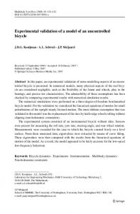
2. Indoor Thermal Response Test (TRT) A thermal response test was conducted in a model chamber filled with homogeneous dry sand, of which a schematic diagram is given in Fig. 1. The experimental setup of the TRT included an electric heater with a circulating pump, a mockup steel box, a water tank, a 4-m length U-shaped Polybutylene (PB) heat

Fig. 1. Diagram for Thermal Response Test and Mockup Steel Box Vol. 18, No. 4 / May 2014

Table 1. Basic Properties of Materials for the Test Specific heat Thermal capacity conductivity (W/m·K) (J/kg·K) a 0.26 835 Joomoonjin Sand b 0.38 525 Polybutylene Pipe Circulating water 0.57 4200 a Measured by Probe test (TP08, Hukseflux) b Given by manufacturer. Materials

Density (kg/m3) 1386.8 955 1000

exchanger, and temperature sensors. Inside the steel box (5 m long, 1 m wide, and 1 m high), the soil could be compacted to a certain density. The steel box was insulated with double layers of 10 mm polyethylene. Besides this, a tent (3 m × 6 m) was installed and a far-infrared radiation heater was operated during the thermal response test to maintain a constant indoor temperature (Fig. 1). A U-type polybutylene pipe (Table 1) (external diameter 25 mm, internal diameter 20 mm, and length 4 m) was installed horizontally in the soil. For the convenience of the experiment, the borehole was not grouted but filled with the sand. The maximum capacity of the heater was 10 kW. Temperature sensors were installed at the inlet and outlet of the GHE pipe, and also buried in the soil 15 cm and 25 cm apart from the center of the PB pipe (Fig. 2). A Korean standard coarse-grained soil, called Joomunjin sand, was used in the test. The physical properties of Joomunjin sand are summarized in Table 2. After sieving (mesh size 3.35 mm), the dry sand was poured into the steel box with a unit weight of 13.97 kN/m3 (with a void ratio of 0.9) in order to carry out the heat flow test in a single layer of soil. Though the ultimate aim of the thermal response test is to estimate the thermal conductivity of the ground, at this point it can also be utilized to calculate the borehole resistance, using

Fig. 2. Two Imaginary Circles Defining Exterior Boundary of Borehole

− 993 −

Gyu-Hyun Go, Seung-Rae Lee, Seok Yoon, Hyunku Park, and SKhan Park

Table 2. Properties of Joomunjin Sand (Yoon et al., 2011) Properties Uniformity Coefficient, Cu Curvature Coefficient, Cc Specific Gravity, Gs Void Ratio, e Maximum Dry Unit Weight, γd (kN/m3) Minimum Dry Unit Weight, γd (kN/m3) Water Content, ω(%)

results, the borehole thermal resistances for Case 1 and Case 2 were estimated to be 1.06 m·K/W and 1.29 m·K/W, respectively. The values of thermal resistance are much larger than that typically found in practice due to the low thermal conductivity of the sand used in the study. In estimating these results, a relationship between heat flow rate and fluid temperature was used, and more detailed information is presented in Table 3.

Value 2.06 1.05 2.65 0.90 16.17 13.49 0.00

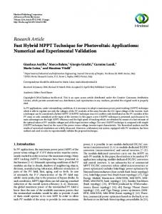
several assumptions. In order to obtain the reference borehole temperatures required for the borehole thermal resistance, two circular boundaries with radii of 0.15 m and 0.25 m were considered to define the imaginary borehole; two RTD sensors were buried at the boundary lines to measure the temperature, as shown in Fig. 2. In general, the difference between inlet and outlet temperature reaches a certain constant value as time goes by, and it is called ‘steady state’ to estimate the long term ground behavior. From an initial ground temperature of 5.85°C, the TRT was performed for about 18 hours with 170 W of heat injection (Q) until the fluid temperature reached a steady state. As shown in Fig. 3, it reached a steady state about 600 min after the start of the experiment, when the heat injection rate of 41.46 W/m was measured. The difference in the fluid temperatures at the inlet and outlet became constant after 600 min. Even though the temperature changes of fluid are occurring in a transient fashion, the gradient of temperature became zero as it reached a ‘steady state’ (Fig. 4b). The difference in fluid temperature between the inlet and outlet, at the steady state, was measured as about 0.5°C (Fig. 3). Fig. 4(a) shows the variation of inlet fluid temperature in the TRT with time, where the final inlet fluid temperature and the mean fluid temperature were 63.42°C and 63.15°C, respectively. Besides this, the measured borehole wall temperatures were 19.29°C for Case 1, and 9.70°C for Case 2. Based on the above

Fig. 4. The Fluid Temperature Variation in TRT: (a) Inlet Fluid Temperature Variation with Time, (b) Gradient of Fluid Temperature with 10 Minutes Time Intervals

Table 3. Comparison of Fluid and Borehole Wall Temperatures and Heat Transfer Rate

TRT Results

Numerical analysis Fig. 3. Difference between Inlet and Outlet Fluid Temperatures − 994 −

Tfluid Tb,av q Tfluid Tb,av q

Case 1 63.15°C 19.29°C 41.46 W/m 63.63°C 18.43°C 43.71 W/m

Case 2 63.15°C 9.70°C 41.46 W/m 63.63°C 8.94°C 43.71 W/m

KSCE Journal of Civil Engineering


3. Borehole Thermal Resistance Estimation Methods

Table 4. Shape Factors for Various Configurations (Remund, 1999) Configuration A B C

3.1 Conventional Series Sum Method In the series sum model, the borehole thermal resistance can be estimated by summing the convective resistance of fluid Rfluid (Eq. (2)), the conductive resistance between pipe and grout Rpipe (Eq. (3)), and the thermal resistance of grout Rgrout (Eq. (4)), as depicted in Eq. (1). Rb = Rfluid + Rpipe + Rgrout 0.023Re Pr λ 1 Rfluid = 0.5 ⋅ ------------ , where hi = -------------------------------------f di πdi hi

(2)

ln ( do ⁄ di ) Rpipe = 0.5 ⋅ -------------------2πλp

(3)

d 1 Rgrout = -----------ln ----b 2πλg de

(4)

n

where do is the outer diameter of the pipe, di is the inner diameter of the pipe, de is the equivalent diameter of the pipe, db is the outer diameter of the borehole, λp is the thermal conductivity of the pipe, hi is the convective heat transfer coefficient of the circulating fluid in the pipe, Re is the Reynolds number of the circulating fluid, Pr is the Prandtl number, n = 0.4 for heating and n = 0.3 for cooling, and λf is the thermal conductivity of the fluid. Usually, the thermal resistance of the grout forms the largest part of the overall borehole thermal resistance, whereas the fluid resistance contributes less than one percent to the overall steady state borehole resistance in a turbulent flow condition (Young, 2001). Therefore, an exact estimate of the grout resistance is crucial for a reliable estimation of the borehole thermal resistance. For the calculation of the grout resistance, various formulas have been proposed, such as Eqs. (5)-(7). Shonder and Beck (1999) applied nd0 as an equivalent diameter (de) in Eq. (4), as shown in Eq. (5), while Gu and O’Neal (1998) used 2d0 Ls ( d0 < Ls < rb ) for de (Eq. (6)) when the shank space Ls is larger than the outer pipe diameter d0 and smaller than the borehole diameter rb, where db is the diameter of the borehole, do is the diameter of the pipe, λg is the thermal conductivity of the grout, and n is the number of pipes.

Fig. 5. Three Different Possible Configurations of U-type GHE in a Borehole

shank distance between pipe legs as an important factor for the estimation of thermal resistance by introducing shape factors β0 and β1, as presented in Table 4, for which the borehole configurations corresponding to cases A, B, and C are shown in Fig. 5. 3.2 Multipole Method The multipole method provides an algorithm to calculate the borehole thermal resistance under a steady-state heat flow condition (Bennet et al., 1987; Claesson and Hellstrom, 2011). It is very useful to consider a composite region (grout and surrounding soil) for calculating temperature fields around vertical GHEs. Eq. (8) explains the temperature fields with heat sources and multipoles. Eqs. (9) and (10) express how to calculate its component and they represent the solutions for heat sources and multi-poles of the order J at z = z n in the composite region. If only a homogeneous medium is considered, the value σ becomes zero, and then Eqs. (9) and (10) could be expressed in much simpler terms.

(5)

(6)

1 Rgrout = ------------------------------βλg β0 ( db ⁄ d0 )

(7)

1

However, the above models oversimplify the multi-legged or coaxial heat exchange pipes into a single pipe. Hence, if the geometry of the pipe arrangement is complex or asymmetric, the above models may not give a reasonable estimation of the borehole thermal resistance. On the other hand, Remund (1999) considered Vol. 18, No. 4 / May 2014

N N J qn T ( x, y ) = Tb, av + Re ⋅ ∑ ----------⋅ W 0( z, zn ) + ∑ ∑ P n, j ⋅ Wj ( z, zn ) 2πλb n=1 n = 1j = 1

⎧ ⎛ rb ⎞ r ⎞, ⎪ ln⎝ -----------⎠ + σ ⋅ ln ⎛⎝ -----------------2 z – z ⎪ n r b – z ⋅ z n⎠ W0 ( z, zn ) = ⎨ ⎪ 1 + σ ⎛ rb⎞ ⎛ rb ⎞ ⎪ ( 1 + σ ) ⋅ ln⎝ -----------⎠ + σ ⋅ -----------ln⎝ ----⎠ z – z 1–σ z n ⎩ 2 b

(8)

z < rb

(9) z > rb

j

d d 1 = -----------ln ----b -----o 2πλg do LS

Rgrout

β1 -0.9447 -0.6052 -0.3796

(1) 0.8

db 1 Rgrout = -----------ln ----------2πλg do n

β0 20.1 17.44 21.91

− 995 −

⎧ rb j ⎛ r pn ⋅ z ⎞ ⎪ ⎛ -----------⎞ + ⎜ -----------------⎟, ⎪ ⎝ z – zn⎠ ⎝ r2b – z ⋅ zn⎠ W j ( z, zn ) = ⎨ ⎪ rpn ⎞ j ⎪ ( 1 + σ ) ⋅ ⎛ ---------⎝ z – z n⎠ ⎩

z < rb (10) z > rb

λb – λ σ = -----------λb + λ

(11)

z = x+y⋅i

(12)


where j is the order of multipoles, J is the number of multipoles, Tb,av is the average borehole wall temperature, qn is the heat flux per unit length of pipe n, λb is the thermal conductivity inside the borehole, λ is the thermal conductivity outside the borehole, Pn, j is the strength of the multipole factor, rb is the borehole radius, rpn is the outer radius of pipe n, and z = x + y ⋅ i represents the complex coordinate. The borehole resistance defines a relationship between heat flow rate and fluid temperature, as depicted in Eq. (13). Thus, once the borehole resistance is determined, fluid temperatures can be estimated with a given borehole wall temperature. In the multipole method, this relationship is represented by Eq. (14) with additional multipole terms. Here, the fluid temperature equation (Eq. (14)) can be derived from Eq. (8). Also, Eqs. (15) and (16) show the components of resistance; the ultimate borehole resistance is finally obtained by superposition of each component. Tfm – Tb, av = Rb ⋅ qn N

Tfm = Tb, av +

(13) ˆ0

∑ qn ⋅ Rm, n + Re ⋅

ρA

where 1--- fD ---------p u u2 indicates the friction heat dissipated due to 2 2 dh viscosity, in which Churchill’s friction model was applied to calculate the fD (Churchill, 1997). Ap is the pipe cross section area (m2), ρf is the fluid density (kg/m3), dh is the mean hydraulic diameter (m), and u is the tangential velocity of fluid (m/s). Also, CP represents the specific heat capacity at constant pressure (J/ kg·K), Tf is the fluid temperature (K), and λf is the fluid thermal conductivity (W/mK). Here, Q represents a general heat source; Qwall denotes a heat source term due to heat exchange with the surroundings through the pipe wall. The equation between pipe flow and heat conduction of solid mass can be coupled through this term; Qwall = hZ ( T ext – Tf) ( W ⁄ m )

where Text is the external temperature outside of the pipe (K), and hZ is an effective value of the heat transfer coefficient; h (SI unit: W/m2·K) times the wall perimeter Z (SI unit: m) of the pipe. For a circular tube, the effective hZ can be denoted such that: 2π ( hZ )eff = ------------------------------------------------------------rn N ⎛ ln --------⎞ r n – 1⎟ 1 1 ----------- + ------------ + ⎜ ------------⎜ λn ⎟ r 0hint rN hext n∑ = 1⎝ ⎠

n=1

N J ⎛ rpn ⋅ zm ⎞ rpn ⎞ j -⎟ - + σ ⋅ ∑ ∑ Pn, j ⋅ ⎜ -------------------∑ ∑ Pn, j ⋅ ⎛⎝ z------------⎠ – z m n ⎝ r 2b – zm ⋅ z n⎠ n = 1j = 1 n = 1j = 1 N

J

j

(14)

m≠n

2 ⎧ ⎛ rb ⎞ rb ⎞ -2 , ⎪ ln ⎝ ------⎠ + βm + σ ⋅ ln ⎛⎝ -----------2 ⎪ r pn r b – r n⎠ 1 ˆR0 = ----------×⎨ m, n 2πλb ⎪ rb ⎞ ⎛ rb-⎞ + σ ⋅ ln ⎛ -------------------⎪ ln ⎝ ------2 ⎝ ⎠ r m, n rb – z ⋅ zn ⎠ ⎩

r pn ⎞ 1 1 - + ----------------Rpn = ----------- ⋅ ln ⎛ ----------------⎝ ⎠ rpn – dpw 2r pn ⋅ hp 2πλp

m=n (15) m≠n

0 where Tfm is the fluid temperature in pipe m, Rˆ m, n is the borehole thermal resistance for J = 0 , Rpn denotes the thermal resistance of pipe n, and dpw is the thickness of the pipe wall. Formulas for the convective heat transfer coefficient hp may be found in the reference of Rohsenhow et al. (1985).

(19)

where rn (m) is the outer radius of wall n, hint and hext are the film heat transfer coefficients inside and outside of the tube (W/ m2·K), and λn is the thermal conductivity (W/m·K) of wall n. Secondly, the heat diffusion equation of solid mass can be expressed as follows. ∂T ext ρi Ci ---------- + ∇ ⋅ ( λi ∇Text ) = Q ∂t

(16)

βn = 2πλbRpn

(18)

(20)

where ρ is the density, C is the specific heat capacity, λ is thermal conductivity. The subscript i denotes each region in which g, c

3.3 Numerical Simulation of TRT The thermal response test was simulated numerically using COMSOL Multi-physics (Version 4.3) with a pipe and heat transfer module. The governing equation for this model is composed of heat equations for conductive and convective heat transfer. First, the heat transfer equation of the flow through a nonisothermal pipe can be expressed as follows (Incropera and DeWitt, 1996; Lurie, 2008). ∂T ρ f Ap C P + -------f + ρ f Ap C P u ⋅ ∇Tf = ∇ ⋅ ( λf AP ∇Tf ) ∂t 1 ρA 2 + --- fD ---------p u u + Q + Qwall 2 2dh

(17) Fig. 6. Convective Heat Transfer Boundary Condition: Energy Balance Around Heat Exchanger − 996 −



Table 5. Comparison of Borehole Thermal Resistances Estimation Methods Experiment Numerical analysis Shonder and Beck Gu and O’Neal Remund Multipole method

Case 1 (K/(W/m)) 1.06 1.03 1.22 0.91 1.00 1.01

Case 2 (K/(W/m)) 1.29 1.25 1.44 1.10 1.19 1.33

Fig. 7. Finite Element Model for Simulation and Specification of Pipe

and s indicate the grout, PHC and bulk soil, respectively. In this study, the described energy balance condition represents a heat transfer boundary condition (Fig. 6). The boundary condition can be expressed by Eq. (18), and effective hZ corresponds to an equivalent convective heat transfer coefficient. Also, the thermal load was not applied to the fluid. It was applied via a temperature boundary, and the used inlet fluid temperatures were obtained from experimental TRT data. Figure 7 shows the finite element model developed for the simulation of the thermal response test. The model has free tetrahedral meshes; maximum element size = 0.5 m, minimum element size = 0.09 m, and maximum element growth rate = 1.5. Material properties used in the simulation are presented in Table 1. The experimental conditions were applied to the numerical model with configuration of Fig. 2. The numerical simulation was performed with the TRT data considering the circulating water flow. The simulated inlet and outlet fluid temperatures around the steady state were 63.87°C and 62.38°C, respectively. This indicated a temperature difference of 0.49°C. The final average fluid temperature was 63.63°C, and the borehole wall temperatures were 18.42°C for Case 1 and 8.94°C for Case 2. Also, the calculated heat flux was 43.71 W/m. Therefore, the borehole thermal resistance was estimated as 1.03 m·K/W for Case 1, and 1.25 m·K/W for Case 2.

4. Results and Discussion By assuming the two imaginary circles (Case 1 and Case 2) shown in Fig. 2 to be the borehole boundaries, the thermal resistances of the boreholes were evaluated based on the series sum model, multipole method, and numerical simulation results. In the estimations using the series sum model and multipole method, the thermal conductivity of the grout was assumed to be Vol. 18, No. 4 / May 2014

Fig. 8. Temperature Fields in Steel Box at Steady State

Fig. 9. Comparison of Results by Multipole Method and Numerical Simulation for Temperature Prediction

the same as that of the soil, because the thermal response test was performed in a homogeneous sand. The sand’s thermal conductivity is presented in Table 1 and its value was determined by a probe test in a dry state. Table 5 compares the experimentally obtained Rb with the analytically or numerically estimated Rb. With reference to the experimental results, numerical analysis and multipole methods predicted an analogous Rb, of which the maximum error was found to be 5% for Case 1, and 3% for Case 2. Also, among the empirical models which were used for the series sum model (Eqs. (5)-(7)), Remund’s models provided the best estimation of Rb for both cases. It is because Remund’s model considers the

− 997 −


Fig. 10. Comparison of Temperature Variations by Experiment and Numerical Analysis: (a) Average Fluid Temperature, (b) Borehole wall Temperature in Case 1, (c) Borehole Wall Temperature in Case 2, (d) Temperature at the Center of Borehole

shank distance in detail compared to other models. Figure 9 shows a comparison of temperature fields at three points in Section A (1.8 m from the top, Fig. 8) using the numerical simulation and Eq. (8) (multipole method). The multipole method tends to overestimate the temperature at the center, and to underestimate it going away from the heat source. Also, as can be seen in Fig. 10, which shows the fluid and ambient temperature variation with elapsed time, the numerical model overestimated the fluid temperature and underestimated the ambient temperature. It could be assumed that this was because the heat from the pipe flow was not totally transferred to the ground in the numerical model which performed the coupled analysis between conduction and convection. However, the difference was so small that it could not be a major problem. On the whole, the numerical results seem to reasonably simulate the actual thermal behavior. Hence, it can be assumed that this numerical model could be utilized for other types of heat exchangers, such as W, 3U and spiral-coil types. Also, the multipole method and numerical model could be applied to estimate the borehole thermal resistance in the composite region by assuming that the inner region of the circular boundaries was filled with grout (λgrout = 2.0). In the analysis, the initial temperature and inlet fluid temperature were set to be identical to those values used in the

Fig. 11. Predicted Temperature Variations Around Grout Borehole

previous analyses. Fig. 11 shows the predicted temperature variation, in which two inflection points can be clearly seen at the exterior boundary of the borehole. In addition, a much higher overall heat injection was predicted than that obtained in the previous analysis. This may be due to the thermal conductivity of the grout, which is greater than that of sand. Certainly, when the thermal conductivity of the soil is changed to that of grout (λgrout = 2.0), it would be expected to show different results. After all, the overall resistance depends on both soil and grout conductivity;

− 998 −



Table 6. Borehole Thermal Resistance in Composite Region λsoil (W/mK)

λgrout (W/mK)

0.26

1.00 1.50 2.02 2.50 3.00 3.50

Rb (K/(W/m)) Numerical analysis Multipole method 0.27 0.28 0.19 0.21 0.15 0.17 0.13 0.15 0.12 0.14 0.11 0.13

if the conductivity of the soil and grout increase, the overall resistance will decrease. Table 6 presents the borehole thermal resistance evaluated from the analysis, in which it can be seen that the multipole method predicted thermal resistance of the borehole slightly larger than that predicted by the numerical models. It is easily seen that the grout thermal conductivity has a great influence on the borehole thermal resistance. However, as can be seen in Table 6, when the thermal conductivity of the grout becomes considerably higher, the borehole thermal resistance will assume a constant value, and then it will be less sensitive to changes in the thermal conductivity of the grout.

5. Conclusions The role of experimentation in this study was to verify the applicability of current borehole resistance estimation models such as the series sum model and multipole method, since this has never before been verified. Also, the numerical model was developed to simulate the test conditions, and after calibration, it was used for a parametric study. However, these cannot be done universally and those results only provide information for the types of shank distance used in the physical model and numerical models. A thermal response test was conducted in a model chamber to measure soil temperature at the boundary lines of imaginary boreholes. The measured results were applied to estimate the thermal resistances of the boreholes. Based on the thermal response test, the validity of the analytical and numerical methods for estimation of the borehole thermal resistance was assessed. For the U-type of GHE, the series model, multipole method, and numerical analysis method reliably estimated the borehole thermal resistance. However, when two or more media are considered, the multipole method and numerical simulation is preferable to estimate the borehole thermal resistance. This is because the empirical models which are used for series sum model actually do not consider the thermal conductivity of the soil in estimating the borehole thermal resistance (Eqs. (1)-(7)). Also, the series sum model may not be practical when the source materials are more than three because it then becomes hard to use Eq. (7). In such cases, the numerical analysis or multipole method appears to have significant advantages. Heat transfer behavior during TRT, for the grouted borehole, was analyzed based on the multipole method and by the Vol. 18, No. 4 / May 2014

numerical simulation. It was found that the grout thermal conductivity has a great influence on the borehole thermal resistance. However, when the grout thermal conductivity becomes considerably higher, the borehole thermal resistance will assume a constant value. Since the numerical results seem to reasonably simulate the actual thermal behavior, it is thought that the numerical simulation model can be utilized for various parametric studies. The ultimate conclusions of this paper can be summarized as follows: 1. With reference to the experimental results, multipole methods and numerical analysis predicted reasonable results. Also, among the empirical models which are used for series sum model, Remund’s models provided a good agreement with the results of numerical analysis and multipole method. 2. The multipole method and numerical simulation verified by experimental data are preferable to estimate the borehole thermal resistance for complex cases of GHEs system because they can be applied regardless of the GHE’s geometry. Furthermore, they are able to estimate the borehole thermal resistance in a composite region considering the two different thermal conductivity. 3. The grout thermal conductivity has a great influence on the borehole thermal resistance. However, when the thermal conductivity of the grout becomes considerably higher, the borehole thermal resistance will assume a constant value, and then it will be less sensitive to changes in the thermal conductivity of the grout.

Acknowledgements This work was financially supported by the Korean Ministry of Land, Transport and Maritime Affairs (MLTM) as part of the UCity Master and Doctor Course Grant Program, and the 2011 Construction Technology Innovation Project (11 Technology Innovation E04) by the Korea Institute of Construction and Transportation Technology Evaluation and Planning, funded by the Ministry of Land, Transport, and Maritime Affairs.

References Bennet, J., Claesson, J., and Hellstrom, G. (1987). “Mutipole method to compute the conductive heat flows to and between pipes in a composite cylinder.” Notes on Heat Transfer 3, pp. 1-42. Churchill, S. W. (1997). “Friction factor equations span all fluid-flow regimes.” Chem. Eng., Vol. 84, No. 24, p. 91. Claesson, J. and Hellstrom, G. (2011). “Multipole method to calculate borehole thermal resistance in a borehole heat exchanger.” HVAC & R. Research, Vol. 17, No. 6, pp. 895-911. Geothermal Design Studio (2007). Ground loop design premier ver. 5.0. user’s manual, USA. Gu, Y. and O’Neal, D. L. (1998). Development of an equivalent diameter expression for vertical U-tubes used in ground-coupled heat pumps, ASHRAE Transactions 104, pp. 347-355. Hellstrom, G. and Burkhard, S. (2000). EED (Earth Energy Designer) user’s manual, Sweden, p. 4.

− 999 −


Incropera, F. P. and DeWitt, D. P. (1996). Fundamentals of heat and mass transfer, 4th Edition, John Wileey & Sons. Liu, J., Zhang, X., Gao, J., and Yang, J. (2009). “Evaluation of heat exchange rate of GHE in geothermal heat pump systems.” Renewable Energy, Vol. 34, No. 12, pp. 2898-2904. Lurie, M. V. (2008). Modeling of oil product and gas pipeline transportation, WILEY-VCH Verlag GmbH & Co., KGaA, Weinheim. Marcotte, D. and Pasquier, P. (2008). “On the estimation of thermal resistance in borehole thermal conductivity test.” Renewable Energy, Vol. 33, No. 11, pp. 2407-2415. Mostafa, H. Sharqawy, Esmail, M. Mokheimer, and Hassn, M. Badr. (2009). “Effective pipe-to-borehole thermal resistance for vertical ground heat exchangers.” Geothermics, Vol. 38, No. 2, pp. 271-277. Remund, C. P. (1999). “Borehole thermal resistance: laboratory and field studies.” ASHRAE Transactions, Vol. 105, No. 1, pp. 439-45.

Rohsenhow, W. M., Hartnet, J. P., and Ganic, E. N. (1985). Handbook of heat transfer fundamentals, New York:McGraw-Hill. Roth, P, Georgiev, A., Busso, A., and Barraza, E. (2004). “First in situ determination of ground and borehole thermal properties in Latin America.” Renewable Energy., Vol. 29, pp. 1947-1963. Shonder, J. A. and Beck, J. V. (1999). “Field test of a new method for determining soil formation thermal conductivity and borehole resistance.” ASHRAE Transactions, Vol. 106, pp. 843-850. Yoon, S., Park, S. K., Park, H. K., Go, G. H., and Lee, S. R. (2011). “Evaluation of heat transfer characteristics in double-layered and single-layered soils.” KSGEE, Vol. 7, No. 2, pp. 43-50. Young, T. R. (2001). Development, verification, and design analysis of the borehole fluid thermal mass model for approximating short term borehole thermal response, Master Thesis, Oklahoma State University, USA.

− 1000 −
