Estimation and propagation of parametric ... - Semantic Scholar

177

© IWA Publishing 2002

Journal of Hydroinformatics

|

04.3

|

2002

Estimation and propagation of parametric uncertainty in environmental models Neil McIntyre, Howard Wheater and Matthew Lees

ABSTRACT It is proposed that a numerical environmental model cannot be justified for predictive tasks without an implicit uncertainty analysis which uses reliable and transparent methods. Various methods of uncertainty-based model calibration are reviewed and demonstrated. Monte Carlo simulation of data, Generalised Likelihood Uncertainty Estimation (GLUE), the Metropolis algorithm and a set-based approach are compared using the Streeter–Phelps model of dissolved oxygen in a stream. Using idealised data, the first three of these calibration methods are shown to converge the parameter distributions to the same end result. However, in practice, when the properties of the data and

Neil McIntyre Howard Wheater Matthew Lees Department of Civil and Environmental Engineering, Imperial College of Science, Technology and Medicine, London SW7 2BU, UK Tel: +44 207 594 6019; Fax: +44 207 823 9401; E-mail: [email protected], [email protected]

model structural errors are less well defined, GLUE and the set-based approach are proposed as more versatile for the robust estimation of parametric uncertainty. Methods of propagation of parametric uncertainty are also reviewed. Rosenblueth’s two-point method, first-order variance propagation, Monte Carlo sampling and set theory are applied to the Streeter–Phelps example. The methods are then shown to be equally successful in application to the example, and their relative merits for more complex modelling problems are discussed. Key words

| calibration, propagation, stochastic, simulation, uncertainty

INTRODUCTION Motivation

1991). The interacting processes and the unknown spatial

The demand for far-sighted, cost-efficient solutions to

and temporal heterogeneities are too many to be accu-

engineering problems has increased simultaneously with

rately modelled or observed. This has forced environ-

our numerical modelling expertise and the sophistication

mental modellers to engage more thought in the procedure

of our computers. Consequently, numerical simulation

of model calibration, and to be more cautious in proposing

models have become an essential part of environmental

deterministic solutions. It is becoming common procedure

and civil engineering. They are routinely used to predict

to include confidence limits with all model results.

the environmental impact of engineering projects, as well

Producing a reliable set of confidence limits on a

as the impact of natural events on our engineering

model result is not difficult, given ideal circumstances. For

achievements.

example, to fit a linear model to observations which are

In the 1970s and 1980s, great attention was given to

normally and independently distributed with constant

improving our knowledge of the underlying environ-

variance requires standard regression techniques, and

mental processes which we aimed to simulate and, as this

derived confidence limits are theoretically sound (see

knowledge grew, the models tended to become complex

Berthouex & Brown 1994). However, the natural environ-

(e.g. Thomann 1998). At the same time, improving

ment is very much non-linear and this biases parameter

environmental databases showed that even theoretically

estimates (e.g. Tellinghuisen 2000). Also, data generally

well founded models failed to accurately replicate obser-

carry sampling and measurement errors and are often

vations (e.g. Bierman & Dolan 1986; see also Binley et al.

unreliable, and, no matter how well behaved the data are,

178

Neil McIntyre et al.

|

Estimation and propagation of parametric uncertainty in environmental models

if the structure of the model is fundamentally wrong then standard regression techniques are flawed. Clearly then,

• •


|

04.3

model structure error (where the model structure is the set of numerical equations which define the

the analysis, as the reliability of the model under new

uncalibrated model),

•

numerical errors—truncation errors, rounding errors

equifinality (Beven & Binley 1992) means that many differ-

and typographical mistakes in the numerical

ent proposed models may appear equally adequate when

implementation,

compared to the data but will give significantly different results when extrapolated to new conditions.

•

2002

model parameter error,

extrapolation of the model into the future also complicates conditions is always in question. The problem of model

|

boundary condition uncertainties.

As reality can only be approximated by field data, data error analysis is a fundamental part of the uncertainty analysis. Data errors arise from:

Scope

•

required spatial and temporal averages),

This paper is a review of methods of uncertainty analysis in environmental modelling. This subject area has pre-

•

ture for additional background and discussion. This paper complements those previous works by taking a demonstrative approach to the review, aiming to give insightful comparisons between the methods using simple examples and theory. As such, it is intended to be a practical guide to the available methods, and to enable and encourage the

measurement errors (e.g. due to methods of handling and laboratory analysis),

viously been reviewed elsewhere (Beck 1987; Melching 1995; Tung 1996) and the reader is directed to this litera-

sampling errors (i.e. the data not representing the

•

human reliability.

Realising that an error-free model would equate to the error-free observations, the relationship between the actual model result M and the actual observations O can be summarised by M − e1 − e2 − e3 − e4 = O − e5 − e6 − e7

(1)

modeller to implement them with forethought, and to interpret the results properly. Notably, this review

where e1–e4 represent the four sources of model error in

excludes methods of recursive parameter estimation (see

the order listed above, and e5–e7 represent the three

Beck 1987) and the use of multi-objective optimisation (see

sources of data error listed above.

Fonseca & Fleming 1995). The utility of these methods is

It is the goal of the modeller to achieve, to within an

evident when the modelling objectives are relatively

arbitrary tolerance, an error-free model by removal of

well defined by observations of the environmental system

e1–e4. However, the modeller is generally neither in con-

(e.g. Whitehead & Hornberger 1984; Gupta et al. 1998).

trol of model structure errors e2, nor numerical errors e3,

Without diminishing the importance of these (and other

nor boundary condition errors e4. Commonly, only the

omitted) methods, this paper is principally concerned with

values of the model parameters are under the direct con-

methods most used for analysis of systems for which

trol of the modeller. The aim would then become one of

supporting observations are relatively sparse.

compensating as far as possible for e2–e4 by identification of the optimum effective parameter values. Central to this paper is the argument that there is always some ambiguity

The sources of uncertainty and their representation in the model

in the ‘optimum’ effective parameter values caused by the unknown natures of, and inseparability of, e2–e7, and that this ambiguity can be represented by parametric

A definition of uncertainty analysis is ‘the means of cal-

uncertainty. As such, the model parameters are used as

culating and representing the certainty with which the

error-handling variables and are identified according to

model results represent reality’. The difference between a

their ability to mathematically explain e2–e7. In most

deterministic model result and reality will arise from:

environmental modelling problems, significant bias in one

179


|



|

04.3

|

2002

or more of these errors will inevitably lead to biased

in environmental modelling (hence the need for uncer-

parameter estimates. While the ideal solution would be to

tainty analysis), and is exacerbated with increasing model

eliminate bias, for example by compensatory adjustments

complexity (e.g. Wheater et al. 1986).

to data or by model structure refinement, such measures

Parameter non-identifiability is caused when the

are often not practical and never comprehensive. In rec-

model has too many interdependent parameters and not

ognition of this, the potential importance of biased model

enough high precision data are available. The problem can

calibration will be illustrated in this paper, and significant

be tackled by collecting additional data and/or by reduc-

attention is given to methods of uncertainty analysis

ing the number of interdependent parameters. Berthouex

which aim to deliver some robustness to bias.

& Brown (1994) observe ‘well-designed experiments will

The difficult task of identifying parameter uncertainty

yield precise uncorrelated parameter estimates with ellip-

is generally approached using methods of calibration

tical joint confidence regions’. This implies that the data

which derive, from the pre-calibration (a priori) parameter

should provide unambiguous information about every

distributions,

distributions

parameter as an independent entity, but in most field

(where, for now, ‘distribution’ is used in the most general

calibrated

(a

experiments this cannot be achieved. Alternatively the

sense). Due to a lack of prior knowledge, the a priori

quote implies that the model should be reduced to a

distributions are often taken as uniform and independent

number of simpler, independent models. While this makes

(e.g. Hornberger & Spear 1980). On the other hand,

the uncertainty analysis straightforward, it may not encap-

the a posteriori distributions, constrained by the data,

sulate all the interdependent processes which the predic-

may be multi-modal and non-linearly interdependent

tive model requires, and may not give insightful results.

posteriori)

(Sorooshian & Gupta 1995). Interdependency arises when

Hence there is need for a compromise between complexity

the model result is simultaneously significantly affected by

and identifiability, consistent with the available data and

two or more parameters, such that the distribution of each

model objective.

parameter must be regarded as conditional on the value of all interdependent parameters. Therefore, it is necessary to refer to the joint parameter distribution, which is defined by a continuous function of all the parameters, and to sampled parameter sets rather than individual parameter values.

APPROACHES TO UNCERTAINTY-BASED MODEL CALIBRATION Calibration is the process of tuning the model by optimisation of the set of model parameters. In traditional

Model identifiability

deterministic modelling, a single optimum parameter set is found such that model results fit the data as closely as

Model identifiability is the extent to which the single most

possible. A variety of automated optimisation procedures

appropriate model can be identified by the modeller. It

are used (see Sorooshian & Gupta 1995). The closeness

includes both model structure identifiability (i.e. that of

of fit is quantified by one or more objective functions

the uncalibrated equations which form the model) and

(OFs). The OF is often some expression of the sum of the

parameter identifiability (i.e. that of the parameter values

squared residuals (of the data and the model result) (see

given one model structure). If a set of field data can be

Weglarczyk 1998). However, the OF should be designed

explained equally well by two or more feasible models,

according to the nature of both the data errors

then the chosen model is poorly identifiable from the data.

(Sorooshian & Dracup 1980; Valdes et al. 1980) and the

As the alternative feasible models will not give identical

model errors (Beven & Binley 1992), as the optimum

results under changed boundary conditions, any predic-

parameter values depend intimately on both. In an

tive results will have implicit uncertainty. Poor identifi-

uncertainty-based calibration, where it is recognised that

ability has been generally identified as a ubiquitous issue

use of one optimum parameter set will give results of

180


|



|

04.3

|

2002

limited insight, the modeller is interested in the response

system response is being modelled and monitored then s2

of the OF over the entire a priori range of parameter sets,

cannot be taken as constant, and Equation (4) becomes

i.e. the OF response surface (see Berthouex & Brown 1994). Analysis of the response surface is the means of deriving the calibrated parameter distributions. This discussion

will

describe

and

demonstrate

different

R

OF = ∏

K

(5)

2 N/2 r = 1 (s r)

where R is the number of responses each measured at N

approaches to this analysis.

locations (in time and/or space). For finding the maximum likelihood, this is equivalent to minimisation of the sum of weighted squared residuals, assuming the responses are

Objective functions and likelihood measures

independent. Similarly, if the variance changes in time

The method of maximum likelihood (see Ang & Tang 1975)

and/or space with the magnitude of the response then

is the basis for traditional calibration, and it is a necessary

an appropriate weighting scheme may be used (e.g.

starting point for this discussion. If the OF is defined as a

Sorooshian & Dracup 1980). For autocorrelated residuals,

likelihood estimator of the model then for each trial model

Romanowicz et al. (1994) describe a suitable likelihood estimator. The OFs in Equations (2)–(5) give the probability

OF = P(e1)P(e2|e1)∏ P[ei|(e1艚e2艚 . . . 艚 e i—1]; i

density of the data sample (say, data sample k) occurring,

i = 3,4, . . . , N

(2)

where ei is the ith of N model residuals (i.e. the difference between the ith of N available data points and the corresponding model result), P(ei) is the probability density of ei, and P(e2ze1) signifies the probability of e2 assuming e1 has already happened. If the N residuals are assumed to be

given the model result. If this model result is defined by a set of parameters (ai) sampled from the a priori joint parameter distribution and applied to a chosen model structure (model structurej), then P[data samplekz(aizmodel structurej)] = OFi.

(6)

independent and normally distributed with zero mean and

This conditional probability may be manipulated using

constant variance s2, and there are F degrees of freedom

Bayes’ theorem (see Ang & Tang 1975) to give the prob-

(i.e. parameters to be calibrated), then Equation (2)

ability of ai given the chosen model structure and given

reduces to

the data sample:

OF =

1 (2ps2)N/2

exp(— 0.5(N — F)).

(3)

P(data samplek)

If N and F are constant, which is likely during a model calibration, Equation (3) is reduced to

OF =

K (s2)N/2

P[(ai|model structurej)|data samplek] × P[(ai|model structurej)

= OFi.

(7)

If only one data sample is considered, with no explicit attention to data sampling error, then P(data samplek) = 1.

(4)

where K is a constant. Therefore, assuming that the sum of

Furthermore, if it is considered that all of S sampled parameter sets have equal a priori probability then P(aiz model structurej) is equal to 1/S. In summary

the squared residuals divided by an arbitrary constant is an unbiased estimator of s2, the least sum of squared residuals maximises the likelihood (Box & Jenkins 1970).

P[(ai|model structurej)|data samplek] =

OFi S

.

(8)

Usually, one or more of the assumptions used in the

The standardised likelihood (so that all the discrete OFs

derivation of Equation (4) is not valid. If more than one

total unity), P′, can be regarded as a point estimate of

181


|



|

04.3

|

2002

probability mass from the a posteriori joint parameter distribution:

P′ [(ai|model structurej)|data samplek] =

OFi ∑OFl

.

(9)

l =1,S

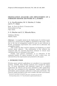
The number of sampled parameter sets, in particular the adequacy of the sampling of the important parameter interactions, is fundamental to the reliability of the results (Cochran 1977; Kuczera & Parent 1998). As the important interactions are not known a priori, the sampling is often randomised, which is known as Monte Carlo sampling (see Ang & Tang 1984). The limitation of this approach is the large number of parameter samples, and hence model runs, generally required to achieve convergence of the a posteriori parameter distribution. However, this can be mitigated by numerous variance reduction techniques, for example Latin hypercube sampling and stratified random sampling (MacKay et al. 1979). Data sampling error arises from the fact that, if many data sets are sampled from the same population, no two sets will give the same likelihood measure for a given model. The data sampling error can be incorporated in the calibration using the theorem of total probability: Figure 1

|

Monte Carlo calibration procedure.

P[(ai|model structurej] = ∑

P[(ai|model structurej|data samplek] ×

(10)

k =1,D

these estimated properties. This is Monte Carlo simulation

P[data samplek])

of data, an established basis for estimation of parameter

where D is the number of sampled data sets. If it is

uncertainty (Rubinstein 1981; Shao & Tu 1995). Such a

supposed that the data sampling error is the main source

procedure is shown in Figure 1. As an alternative to

of uncertainty, and only the maximum likelihood model

simulation of data, residual bootstrapping can be used

for each data realisation need be considered, then P[a′kzmodel structurej] = P[data samplek]

(e.g. Shao 1996). This uses sub-samples of the residuals (of the available data and the maximum likelihood model (11)

where a′k is the maximum likelihood set of parameters set found for the kth sample of data. Thereby, many different data sets from the same population are required, usually

result) as the kth data realisation. As with Monte Carlo simulation of data, residual bootstrapping requires initial assumptions about the maximum likelihood, but it avoids assumptions regarding the variance.

an unrealistic requirement in the context of environmental sampling programmes. Alternatively, one available sample can be used to estimate the distributional properties of the

Possibility theory and the HSY method

residuals (e.g. Ang & Tang 1975). Equation (11) can then

A problem with the maximum likelihood estimator is that

be solved by randomly simulating data on the basis of

simplifying assumptions are required about the nature of

182


|



|

04.3

|

2002

the data errors. In environmental monitoring, the sam-

which may include analysis of available data. The result of

pling location and methods of measurement generally

this approach to calibration is an a posteriori sample of

cause unknown biases in the maximum likelihood esti-

equally possible parameters and a complementary sample

mate. Various methods may be tried to improve robustness

of impossible parameter sets. Van Straten & Keesman

to assumptions regarding data bias. One approach is to use

(1991) demonstrate how the a posteriori sample of possible

possibility theory (Zadeh 1978; see also Wierman 1996). A

parameters can be propagated to a range of possible

possibility distribution describes the perceived possibility

results. Statistical comparison of the contents of these

of an event where the maximum possibility is 1 and the

sets can robustly quantify model sensitivity to individual

minimum is 0. In possibility theory, the rules of union and

parameters (e.g. Spear & Hornberger 1980; Chen &

intersection differ from those in probability theory. For

Wheater 1999), and so the method is often referred to as

independent, random variables X and Y,

Regional (or Global) Sensitivity Analysis. After Beck (1987), the method is referred to hereafter as the

Possibility(X∩Y) = Minimum

[Possibility(X),

Possibility

(Y)]

(12a)

Possibility(X∪Y) = Maximum

[Possibility(X),

Possibility

(Y)]

(12b)

Hornberger–Spear–Young

(HSY)

algorithm

and

an

interpretation of the algorithm is illustrated in Figure 2.

Generalised Likelihood Uncertainty Estimation (GLUE) Beven & Binley (1992) developed the HSY method into

Applying possibility theory to model calibration requires a

their Generalised Likelihood Uncertainty Estimation

subjective measure of the possibility of the outcome of each

(GLUE), so that every possible model was weighted with a

candidate model. Using Equation (12a), for example, the

likelihood. The array of likelihoods (for each model struc-

possibility of any model result is the model residual (out of

ture) is interpreted as point estimates of probability from

all N model residuals) perceived to be the least likely.

the joint parameter distribution for that model. As new

Although the significance of the remaining N − 1 residuals

data becomes available, the distributions can be updated.

would be lost, the robustness to data bias would be

The predictions from alternative model structures with

increased by avoidance of the multiplicative likelihood

their own joint parameter distributions can be combined

estimator.

using Bayes’ method. The key feature of GLUE is that the

Another particular appeal of applying possibility

modeller designs an OF which is taken as a measure of the

theory to model calibration is that it provides a convenient

likelihood. It is emphasised that the estimated uncertainty

basis for calibrating the model using subjectively defined

depends largely on the user’s design of likelihood measure

support criteria. While such reasoning can be based on

(e.g. Freer et al. 1996), and that the basis of the design

interpretation of data it may also be knowledge-based.

should be explicit. In particular, the GLUE likelihood

That is, the possibility of any candidate model can be

measure should not be interpreted as a statistical likeli-

judged

non-

hood estimator, as used in Equations (2)–(5), unless it is

documented) knowledge about the environmental system

on

the

basis

of

non-numeric

(even

specifically designed as such (e.g. Romanowicz et al. 1994)

rather than by ‘hard’ data.

with regard to the data and model errors.

Hornberger & Spear (1980) suggested a groundbreak-

A major problem with the likelihood estimators of

ing approach to calibration of environmental models

Equations (2)–(5), which may be addressed using GLUE,

which has distinct parallels with possibility theory. In

is the assumption that the model is correct and uncertainty

their method, an a priori parameter set, applied to a

only arises from the statistical significance with which the

given model structure, is considered to be a possible model

data can define the optimum solution. If the model is

of the system if the corresponding model result lies

biased with respect to the observations (i.e. incapable of

wholly within a set of characteristic system behaviour. The

producing uncorrelated residuals), this has the unsatisfac-

characteristic behaviour is defined by subjective reasoning

tory effect that the parameter uncertainty tends to reduce,

183


|



|

04.3

|

2002

stochastic model may be judged by its ability to encompass the measurements, irrespective of the measurement errors. However, simple manipulation of likelihood estimators will not solve the problem of model or data bias, for which GLUE must be used in its more general, subjective capacity.

Adaptation of parameter distributions It has been described how the OF evaluated for any parameter set can be interpreted as a point estimate of probability mass or possibility. Thus, using Monte Carlo simulation of the parameters, a response surface equivalent to an a posteriori distribution can be approximated. However, many thousands of a priori parameter samples may be required for an adequate approximation to be made (e.g. Kuczera & Parent 1998). To improve the efficiency of the calibration, attempts have been made to adapt the a priori distribution to an a posteriori form. Such approaches are commonly called adaptive random searches (ARSs). Types of ARS include genetic algorithms (Holland 1975), shuffled complex evolution (Duan et al. 1993) and Monte Carlo Markov chains (see Rutenbar 1989), all of which have proved useful for environmental model calibration and for uncertainty analysis (e.g. Mailhot et al. 1997; Mulligan & Brown 1998; Figure 2

|

HSY calibration procedure.

Thyer et al. 1999). Careful thought is required before applying an ARS to estimation of parametric uncertainty because the achieved a posteriori distribution depends on the particular ARS and the convergence criteria, as well as the data, the model and the OF. So, while a

as high likelihood is exclusive to those parameter sets (of

distribution representing uncertainty may be derived,

course, themselves biased) which compensate for the

the significance of this uncertainty is not necessarily

model bias. Furthermore, when the number of data points

helpful.

is high, parameter uncertainty is low and the associated

Here, a Monte Carlo Markov chain model proposed

confidence limits on the model results will not encompass

by Metropolis et al. (1953) is described. The algorithm uses

many measurements of the real system. This may be solved

a Markov chain process (see Rutenbar 1989) which, in

within the GLUE framework, for example, by prescribing

essence, assumes that the current state of a system dictates

a value of N (Equations (3)–(5)) which is less than

the probability of moving to any proposed new state. The

the number of data points, so increasing the parameter

Metropolis algorithm was originally developed to simulate

variance (e.g. Freer et al. 1996). This has a distinct advan-

the stochastic behaviour of a system of particles at thermal

tage in regulation-driven modelling exercises, where the

equilibrium. Applied to model calibration, it adapts the

184


|



|

04.3

|

2002

population of parameters until the OF (in this case to be minimised) is described by the distribution

P(ai) =

1 KMET

e— OFi /A

(13)

where KMET is a standardisation constant such that the total of all P(ai) is unity, A is a case-dependent constant and ai is the ith parameter set in the derived population. Note that, while the distribution of the accepted OFs converges to the Gaussian form of Equation (13), the distribution of the accepted parameter sets depends upon the relationship between the model and the OF. The algorithm starts from an arbitrary location in the a priori parameter space. From then on, the probability of any sampled parameter set ai being accepted into the population depends entirely on comparison of OFi with that of the last accepted set, OFi − 1. This probability is defined by Equations (14a) and (14b):

P(ai—1ƒai) =

= exp

&

P(ai) P(ai—1)

OFi—1 — OFi A

/

P(ai—1ƒai) = 1

for

OFi—1 < OFi

(14a)

for

OFi—1 ‰ OFi .

(14b)

Each parameter set is sampled at a random distance and direction from the previously added set, subject to the a

Figure 3

|

Metropolis calibration procedure.

priori constraints and a specified maximum distance, B. An implementation of the Metropolis algorithm is suggested in Figure 3. Mailhot et al. (1997) and Kuczera & Patent (1998) find the Metropolis algorithm to be useful in uncertainty analysis. The Metropolis algorithm can be refined by allowing constants A and B to be updated at intervals, thereby gradually increasing focus on the optima.

section which discusses the example in the context of more complex and practical problems. A steady state model of organic carbon (BOD) decay and dissolved oxygen (DO) in a river can be described by the Streeter–Phelps equations (Streeter & Phelps 1925): (x/n)

Example of calibration This example aims to demonstrate some of the above approaches to the estimation of a joint a posteriori

BODx = BOD0e — koc koc }BOD0 — koc(x/n) (x/n) — e — kau DOx = DOsat — [e ]— kau — koc (x/n)

(DOsat — DO0)e — kau

(15a)

(15b)

parameter distribution, and establish some relationships

where koc is the BOD decay rate, kau is the oxygen

and contrasts between them. To make the demonstration

aeration rate, x is the distance downstream from a point

manageable, the model is simple and the data are ideal-

pollution source, DO0 and BOD0 are the respective con-

ised. Attention is drawn to the last paragraph in this

centrations in the river at x = 0, v is the average transport

185


Table 1

|

|


Value

04.3

|

2002

Unit

koc

1

d−1

kau

5

d−1

75

mgO/l

DO0

0

mgO/l

DOsat

12

mgO/l

v

|

Deterministic parameter values for Streeter–Phelps example

Parameter

BOD0


0.5

m/s

velocity and DOsat is the concentration of DO at saturation. Synthetic data are generated by the model using the parameter values and boundary conditions in Table 1, and random errors are introduced in DO( = eDO) from an N(0, 22) population, and in BOD ( = eBOD) from an independent N(0, 102) population. With 20 data locations spaced at 5 km intervals along a 100 km stretch of river, the synthetic data are illustrated in Figure 4. These data, together with the maximum likelihood model solution, are used to estimate the properties of the distribution of

Figure 4

|

Synthetic data for Streeter–Phelps model.

residuals, which are listed (alongside the population properties) in Table 2. This estimation is based on the convergence properties of a sample’s maximum likelihood and variance using the Central Limit Theorem (from Ang &

population distribution kept the same. The comparison of

Tang 1975). Assuming v and the boundary conditions are

calibrated marginal distributions is shown in Figure 5.

known, the parameters to be calibrated are koc and kau.

Figure 6 gives a similar comparison of the marginal distri-

The synthetically derived error population is ran-

butions, this time changing the data quality (i.e. varying

domly sampled and Monte Carlo (MC) calibration of

the expected standard deviation shown in Table 2). Note

parameters koc and kau proceeds as described in Figure 1.

that the distributions of koc and kau are correlated (cor-

The maximum likelihood set (koc, kau) is found for each

relation coefficient = 0.31), meaning that the a posteriori

data sample using stratified random sampling, using

model must be defined by the bivariate distribution of koc

the least sum of squared objective function defined in

and kau as opposed to the marginal distributions shown in

Equation (5). One thousand samples of the a priori

Figures 5 and 6. Note also from Figures 5 and 6 that the

parameters are used to estimate the optimum parameter

‘true’ values of koc and kau (1 and 5, respectively) do not

set for each of 200 realisations of the data. That is, 0.2

necessarily correspond to the identified maximum likeli-

million model runs are used to derive the posterior

hood (see especially the result for 5 data locations in

parameter distributions. This exercise is repeated with

Figure 5). This is because the available data, upon which

different quantities of synthetic data (i.e. varying the

the MC calibration is founded, are only a sample of the

20 locations shown in Figure 4), with the data error

true water quality.

186


Table 2

|

|


|

04.3

|

2002

Properties of the DO and BOD data error population Property of

BOD

DO

Figure 5


|

Standard deviation

residuals

Population

Sample

of sampled property

Mean

0

0

2.14

Standard deviation

10.00

9.69

5.39

Mean

0

0

0.43

Standard deviation

2.00

2.17

0.87

Calibrated distributions with different sample sizes.

Figure 6 shows that MC gives a significantly uncertain

laboratory errors, or simply because of physical con-

value for the parameter kau despite perfect data, which is

straints such as a lower bound of zero. To explore the

contrary to intuition. This implies that adequate conver-

effect of this, the DO data are raised by a random amount

gence of the joint parameter distribution has not been

between 0 and 5 mgO/l, and to a minimum of zero and the

achieved using 0.2 million model runs. Whether this is

maximum of DOsat. The calibration is done as before, with

primarily due to the inefficiency of SRS as an optimisation

20 data locations, and the calibrated parameter distri-

procedure, or due to the limited number of realisations of

butions are shown in Figure 7. This shows that where

the data, is not investigated here. However, it is clear

significant bias is suspected but unknown, another

that the difficulty of achieving convergence, even for a

approach to calibration is required. Note that the par-

relatively simple problem such as this, contributes to the

ameter uncertainty associated with kau is implied to be

approximate nature of the solution.

significantly reduced, contrary to what we would desire. In

It is common in environmental monitoring that data

practice, model structure error is particularly relevant to

are biased descriptors of the true state of the environment.

the Streeter–Phelps model, because it neglects many of the

This may be because of heterogeneity which is not recog-

complexities of pollution transport and decay. The effect

nised in the sampling programme, or because of repeated

of model structure error is similar to that of data bias (at

187


|


Figure 6

|

Calibrated distributions with different error variances.

Figure 7

|

Effect of BOD error bias.


|

04.3

|

2002

least in this case), in that it biases parameter estimates and

dom sampling (SRS) gives some control of the location of

causes inappropriate reduction in parameter uncertainty.

the point estimates and so coverage of extreme values is

It has been shown how MC simulation can be used to

assured. Here, GLUE is applied to the previous Streeter–

derive the calibrated marginal parameter distributions by

Phelps example using the data sample illustrated by Figure

frequency analysis of the sampled maximum likelihood

4. The likelihood function defined in Equation (5) is

parameters. GLUE offers the opportunity to reduce the

applied (whereby for this example we are opting not to

computation required by not explicitly accounting for the

explore the full generality of GLUE; instead we are main-

data sampling error. It is based on point estimates from the

taining a strictly statistical likelihood estimator), using a

joint distribution which are directly applied to uncertainty

total of 2000 random samples of (koc, kau). The likeli-

propagation and, therefore, the non-linear parameter

hood equipotentials of the derived point estimates are

dependencies are implicitly handled. Also, stratified ran-

shown in Figure 8. For comparison with the MC results,

188


|



|

04.3

|

2002

mum likelihood as normally distributed with variance s2m/N (assuming that sm is accurate, see Ang & Tang 1975):

P′ MC =

N0.5

1

exp[— 0.5d2N/sm2].

KMC (2psm2 )0.5

(17)

As it is known that the integrals of Equations (16) and (17) are both unity, to prove that they give the same result for all parameter samples only requires that the ratio P′GLUE:P′MC is proven to be the same for all d:

P′ GLUE P′ MC

=

KMC

(2psm2 )0.5

KGLUE (2p(sm2 + d2))0.5N N0.5

×

exp[— 0.5(N — F)] exp[— 0.5d2N/sm2] Figure 8

|

(18)

.

Equipotentials of point estimate likelihoods using GLUE.

Amalgamating all terms which are independent of d into one constant K:

P′ GLUE the marginal distributions of koc and kau are illustrated in Figure 9. Repeated for other data scenarios, the results are summarised in terms of calibrated parameter variances in Figure 10.

P′ MC

=K

fi

exp(d2/sm2 ) (sm2 + d2)

^

0.5N

.

(19)

Expanding the exponential term into a MacClaurin series, and neglecting terms higher than quadratic, gives,

The similarity of the GLUE and MC results is striking, considering that the GLUE method does not explicitly account for data sampling error, and has reduced the

P′ GLUE

computation from 0.2 million to 2000 model runs. The

P′ MC

K =

&

sm2 + d2

/

0.5N

(sm

sm2 2 + d2)0.5N

=

K smN

(20)

theoretical basis for the similarity can be demonstrated at which is constant for all d. Thus it is shown that Equations

a simple level. Equation (3) is re-expressed as

(16) and (17) are describing the same probability distri-

P′ GLUE =

1

bution if d4/s4m and higher-order terms can be neglected.

1

KGLUE (2p(sm2 + d2))0.5N

exp[— 0.5(N — F)]

(16)

These terms are not negligible if N is very low, but in such cases the assumptions underlying Equations (16) and (17)

where P′GLUE is the probability of any parameter set, d2 is

are not justifiable anyway. Nevertheless, the theory

the variance of the corresponding model result around the

presented here supports the experimental results in

2 m

is the error variance

Figures 9 and 10, and confirms that GLUE is (usefully)

around the maximum likelihood result and KGLUE is a

neglecting higher-order uncertainties in this application.

maximum likelihood result, s

′ MC

is

Interestingly (but probably not of practical value),

the probability of any parameter set, but d2 is the

Equation (19) provides a basis for exactly reproducing the

variance of the maximum likelihood result for any data

MC result by adjusting the GLUE result.

standardisation constant. In the MC method, P

realisation around the result for the available data

The Metropolis algorithm (Figure 3) is observed to

sample. Approximating the standard error of the maxi-

further increase the efficiency (in terms of time for

189


Figure 9

|

|


|

04.3

|

2002

Comparison of calibrated parameters using GLUE and MC.

convergence of the (koc, kau) covariance matrix) of the Streeter–Phelps calibration by up to 60%. The OF is

P′ MET =

defined as the sum of the variance-weighted squared errors, i.e.

OF =


1

= 20

∑ e 2i,DO +

s2m,DO i = 1

1

20

∑ e 2i,BOD

s2m,BOD i = 1

=

(21)

where sm,DO and sm,BOD are the error population stan-

1 KMET 1 KMET 1 KMET

OFi

& A/ (d + s )N exp — fi s A ^ d N s N exp — exp — fi s A^ fi s A^.

exp —

2

2

m 2

m

2

2 m 2 m

2

m

(22)

Equating this with (17) gives

dard deviations (from Table 2), and ei,DO and ei,BOD are the ith residuals of DO and BOD, respectively. Then, the

1

probability of selecting parameter set ai pursuant to ai − 1

KMET

is given by Equation (14). A is specified as 2, and the

1

maximum permitted step, B, is specified as (Bkoc = 0.05, Bkau = 0.25). The data set illustrated by Figure 4 is used.

fi

exp —

d 2N sm2 A

N0.5 2 )0.5

KMC (2psm

exp

^ fi

exp —

fi

—

sm2N sm2 A

0.5d2 N sm2

^

^= (23)

The converged koc and kau distributions are almost iden-

and equating the exponents with the d2 terms gives A = 2.

tical to those obtained using the MC method (Figure 9)

The specification of A and the OF used here is generally

and Figure 10 supports this result under a range of data

applicable to an approximation of the standard error of a

conditions. All the Metropolis results are reproducible

maximum likelihood model result assuming Gaussian

with different values of B, although the most efficient

error. As sm is not generally known a priori, updating of A

depends on the convergence criterion. From Equation

within the algorithm may be useful. Also, A and the OF

(13) it is clear that the Metropolis result is sensitive to A,

can be designed to give a more useful representation of

and it is not a coincidence that this choice of A almost

uncertainty than the standard error, with broader confi-

replicates the MC result. Idealising Equation (21) by con-

dence intervals to reflect, for example, unknown model

sidering a single response, and using the definitions for

and data bias. Whether this can be done in a robust and

Equations (13) and (16):

meaningful way is a matter for further research. While

190


Figure 10

|

|



|

04.3

|

2002

Comparison of calibrated parameter variances using GLUE, MC and Metropolis.

Metropolis is an adaptive search, and therefore potentially

defined by Equation (24a) is represented in Figure 11. Note

superior to GLUE for finding the maximum likelihood and

that, as opposed to Figure 8, the set limits defined in Figure

variance, its sampling of the extreme values is relatively

11 are not smooth due to the discontinuous nature of

sparse.

Equation (24). The HSY method is potentially more robust

Now consider the HSY method of Hornberger &

to model error and data bias than statistically based likeli-

Spear (1980). A set of characteristic system response is

hood methods because unreliable results, such as those

defined, with the sampled parameter set given a possibility

illustrated in Figure 7, can be avoided with appropriate

of 1 (P(d) = 1), if the model result falls wholly within

specification of the upper and lower bounds of characteristic

pre-specified lower and upper limits. For the Streeter–

response. Of course, improvement in reliability is at the

Phelps example, those limits are of DO and BOD (DOl,

expense of a less specific description of uncertainty.

DOu and BODl, BODu, respectively), i.e.

Notwithstanding its demonstrative limitations (see below), this example compares classical Monte Carlo

P(d) = 1 for DOl < DO < DOu∩BODl < BOD < BODu

(24a)

simulation, GLUE and Metropolis and shows that these methods are not fundamentally different insofar as they

P(d) = 0 for all other results

(24b)

can produce the same calibration results, given consistent objective functions. The question of which is more ef-

For example, if the upper and lower limits are taken to be the

ficient depends upon the case. Monte Carlo sampling of

90% confidence limit defined by the data sample and its

the data is a rigorous method of sampling from a known

maximum likelihood model result, the set of (koc, kau)

error distribution, and can be modified to a resampling

191


|



|

04.3

|

2002

illustrated by Figure 8, is well behaved. Many practical problems involve multi-modal responses together with discontinuities derived from the discontinuities in the model structure, again increasing the difficulty of convergence. Thirdly, Equation (15) is an analytical solution to the Streeter–Phelps model, which is solved easily and quickly, which facilitates Monte Carlo methods. Models of the environment are more often in the form of systems of differential equations for which approximate numerical solutions are required and computational demands are relatively high. While computer power is continuously increasing and parallel processing facilities are available, computation time remains a limitation in model calibration and uncertainty analysis. Lastly, the data have been synthesised from a normal population of residuals which are uncorrelated and have zero mean. Only a nomiFigure 11

|

The (koc, kau) uniform possibility distribution.

nal look at the effects of data bias has been included.

scheme if the error distribution is unknown. GLUE avoids sampling of data and, if used with statistical likelihood

UNCERTAINTY PROPAGATION

estimators, can be an extremely good approximation to the

Uncertainty propagation in this context means propa-

more rigorous data sampling schemes. In addition, it has

gating the calibrated parameter joint distribution to a

more general application than used in the example (see

stochastic result. Methods of propagating probability dis-

below). Metropolis has the advantage of adapting the

tributions can be classified as sampling methods, variable

response surface, thereby generally locating the parameter

transformation methods, point estimation methods and

set mode(s) to within some tolerance in a shorter time.

variance propagation methods. An alternative to prob-

However, this is at the expense of the reliability of extreme

ability theory is the theory of possibility (Zadeh 1978).

results. All these approaches to calibration require careful

Each of these approaches is discussed here. In this dis-

design of the OF, as this defines the variance of the a

cussion, the general term ‘random variables’ includes

posteriori joint parameter distribution. The HSY algorithm

uncertain parameters, boundary conditions and stochastic

was briefly explored, and it was shown how it might be

results.

used to cover for the effects of model and data biases, at the cost of a less discriminating description of uncertainty. With regard to more complex and more realistic environmental modelling, the above example has several

Monte Carlo methods

important limitations. Firstly, it only has two interdepend-

Monte Carlo (MC) simulation applied to uncertainty

ent parameters, while many models have significantly

propagation means generating discrete parameter sets

more. In such cases converging the a posteriori joint

according to their probability or possibility distribution,

distribution would be expected to be much more difficult,

and running a simulation using each set. Alternatively, the

perhaps requiring many thousands of model runs (e.g.

population or point estimates which were derived during

Thyer et al. 1999), depending on the strength and nature of

calibration can be recalled, thereby avoiding the need for

the interactions. Secondly, the response surface, which is

assumptions regarding the form of the distribution. The

192


|



|

04.3

|

2002

results of multiple simulations give a close approximation

Rosenblueth’s point estimation method for symmetric

to the analytical form of the probability density function

and non-symmetric variable distributions (Rosenblueth

(PDF) using frequency analysis, and any model can be

1981) aims to reduce the computational demands of vari-

easily included in such a framework with minimal input

ance propagation by eliminating the calculation of deriva-

from the modeller. For these reasons, MC is a well used

tives. The PDF of each random variable is represented by p

method of uncertainty propagation. The main disadvan-

discrete points, located according to the first, second and

tage of MC is that a great number of model runs may be

third moments of the PDF. The joint PDF of F random

required to reliably represent all probable results,

variables is represented by the array of projected points.

especially when there is a number of random variables.

Therefore, pF points are used. Each point is assigned a

Methods of estimating a preferred number of samples are

mass according to the third moment and the correlation

available (e.g. Cochran 1977), although this also depends

matrix. All points are propagated discretely to pF solutions

on the convergence or divergence during propagation and

and the first moment is the weighted average; the second

therefore is case specific (Tellinghuisen 2000). Variance

moment, that of the squares; and the third moment, that of

reduction techniques, such as stratified random sampling

the cubes. Most usually a two-point scheme is used

(SRS) and Latin hypercube sampling (see MacKay et al.

whereby 2F points are required. For symmetrical distri-

1979), are often used to improve efficiency.

butions for F > 2, the number of evaluations can be reduced from 2F to 2F by using Harr’s point estimation method (Harr 1989). Harr’s method is a useful improve-

First-order and point estimate approximations

ment on Rosenblueth’s, but is limited by the necessity of

First-order variance propagation is the most common

symmetrical distributions. A similar approach which

method of uncertainty propagation (Beck 1987). If a func-

allows for skewed distributions but not correlations is

tion Z = f(X), X = (x1, x2, . . . xF) is approximated by a

described by Hong (1998). Protopapas & Bras (1990) have

first-order Taylor series expansion around the expected X,

applied Rosenblueth’s two-point method to a rainfall-

mx, then

runoff model and Yeh et al. (1997) have similarly applied Harr’s method, and a useful review of all these point

mZ = f(mX)

(25a)

s2Z = ∆(Z)T Ψ(X)∆(Z)

(25b)

estimate methods is given by Christian & Baecher (1999). It is worth noting that some Monte Carlo-based methods of calibration, for example GLUE (Beven & Binley 1992), are randomised point estimate methods. In GLUE, many random samples of the a priori parameter

where ∆(Z) is the F × 1 matrix of derivatives of Z with

space are assigned GLUE likelihoods, which then become

respect to X; j(X) is the F × F covariance matrix of (x1, x2,

point estimates for the uncertainty propagation stage.

. . . xF) and mZ and s2Z are the mean and variance of Z. This

Unlike Rosenblueth’s method, it is generally assumed that

is a linear approximation of uncertainty propagation

there are enough points to derive the model output PDF,

which is only completely reliable for linear models. The

not just the lower moments.

accuracy of this method for non-linear models can be improved by using a higher-order Taylor series expansion, but this becomes computationally demanding, especially if the derivative values are calculated numerically. Variance

Possibility theory

propagation is a useful method for models which can

Possibility theory (Zadeh 1978) offers a robust alternative

approximated by quasi-linearisation (see Gelb 1974), i.e. a

to propagation of probability distributions. To illustrate

series of localised linear functions. For example, Kitanidis

this, let f(X, Y) be a function which is strictly increasing or

& Bras (1980) applied variance propagation to a quasi-

decreasing with respect to both variables X and Y, and let

linearised hydrologic model.

X and Y have possibility distributions which rise internally

193


|



|

04.3

|

2002

to a single peak or plateau. Then, using the rules of possibility in Equations (12a) and (12b), the two values of X( = xlp, xup) and Y( = ylp, yup) with possibility P (commonly called the P-level a-cut of X and Y) define the two values of f (X,Y) with possibility P. For example, if ∂f/∂X is positive for all X and ∂f/∂Y is negative for all Y, then f(X,Y)up = f(xup,ylp)

(26a)

f(X,Y)lp = f(xlp,yup)

(26b)

This method can be extended to problems with many uncertain parameters so long as the aforementioned ‘increasing–decreasing’ and ‘single-peak’ conditions are met for each. While an infinite number of a-cuts are required for the exact solution to non-linear propagation (Wierman 1996), an approximation of the propagated possibility distribution can be made with a small number of computations. The associated difficulties and limitations should be recognised. Firstly, special attention must be given to the method of calibration in order to derive meaningful parameter possibility distributions. Secondly, the possibility is greater than the probability at all points (Zadeh 1978), and so the former is a less specific descriptor of uncertainty. Thirdly, if parameter a-cuts are

Figure 12

|

Propagated uncertainty for Streeter–Phelps model.

to be used, prior knowledge of the sensitivity of the results to the parameters is required. Lastly, there remains the problem of parameter interdependence which, as in probability theory, complicates the analysis, generally requir-

three alternative methods give (practically) identical

ing that the P-level a-cut be defined by a large sample of

results for the first three moments. The numerical

parameter sets.

efficiency of the first-order variance and Rosenblueth twopoint methods is proven, despite the apparent nonlinearity of the model with respect to koc and kau. In fact,

Propagation of the Streeter–Phelps model parameters

the model is only significantly non-linear at low values of DO, and the performance of the first-order method

The joint (koc, kau) distribution previously identified

deteriorates with either increased BOD loading or

using GLUE (Figure 8) is propagated to give spatially

increased data uncertainty. Propagation of the possibility

varying distributions of BOD and DO. Again, the bound-

distribution illustrated in Figure 11 replicates the 90%

ary conditions defined in Table 1 are used. Firstly, each of

confidence limits derived using the other methods (assum-

the 2000 point estimates of (koc, kau) is propagated

ing normality), although this result is specific to the

through the Streeter–Phelps model, then the first-order

definitions used in the derivation of Figure 11 (see

variance and Rosenblueth two-point methods are applied,

Equations (24a,b)). None of the methods can reproduce

using the covariance matrix of (koc, kau) which is derived

the 90% confidence limits on the data error upon which

from the GLUE point estimates. It is observed that the

the calibration was founded, illustrated in Figure 12.

194


|



|

04.3

|

2002

Results are constrained by the boundary conditions, irre-

be said that the natural environment is too complex, with

spective of parameter uncertainty. Therefore, if they are

too many heterogeneities and apparently random influ-

not precise, the modeller must treat the boundary con-

ences, to be usefully described without including some

ditions as random variables as well as the parameters.

estimation of uncertainty. The inclusion of uncertainty

Furthermore, it may be observed from Figures 4 and 12

analysis adds to a conventional modelling exercise in two

that the 90% confidence limits contain much less than

main ways. Firstly, the calibration of model parameters

90% of the data. Using the multiplicative likelihood esti-

involves identification of parameter distributions rather

mator of Equation (5) has meant the limits represent the

than single parameter values. Secondly, the parameter

uncertainty in the maximum likelihood solution, not the

distributions (and alternative model structures if used) are

variance of the data.

propagated to stochastic rather than deterministic results.

The example of the Streeter–Phelps model has illus-

A variety of applications of Monte Carlo (MC) simu-

trated that alternative methods of estimation and propa-

lation can provide detailed information about the cali-

gation of parametric uncertainty can lead to practically

brated parameter distributions. A traditional application

the same result. However, the example is too simple to

of MC simulation is to optimise the parameters with

fully show the limitations of the reviewed methods. At the

respect to each of a multitude of realisations of the data,

calibration stage, unknown model structure and data bias

thereby giving a sample of optima. If data are of limited

may mean that statistical interpretation of the model

quality, this sample converges slowly, and reliable

residuals is not useful, and a more robust approach must

results may not be achieved within an acceptable time.

be sought, by subjective evaluation. At the propagation

Generalised Likelihood Uncertainty Estimation (GLUE)

stage there may be strong non-linear dependency of par-

requires the modeller to design a likelihood measure

ameters, which must be approximated by a covariance or

which is used in the calibration. This design may be based

correlation coefficient in Rosenblueth’s method and the

on classical likelihood estimators, in which case GLUE is

first-order variance method, leading to a poor approxi-

seen to significantly improve the efficiency of traditional

mation of prediction uncertainty. Practical environmental

MC simulation while giving similar results. Alternatively,

models often include cyclic, non-continuous or otherwise

the GLUE likelihood measure may include subjective

highly non-linear processes which will test all methods

interpretation of the data as well as the potential for model

much more severely than was attempted here. Practical

structure error, in order to give more robust results. GLUE

models may take considerable processing time and have

is founded on the principles of Bayesian estimation, and in

many uncertain parameters. Achieving reliable results

this regard is especially useful for updating model uncer-

using MC simulation may be computationally expensive,

tainty estimation as new data, knowledge and models

although this is of less concern where parallel processing

come to light. The Metropolis algorithm is a Monte Carlo

facilities are available.

Markov chain procedure which has proven useful in parameter uncertainty estimation. In some cases it is a more efficient method of deriving parameter distributions than GLUE, although it cannot give such detailed information about extreme values. The theoretical and practi-

CONCLUSIONS Review summary

cal similarity of the traditional MC, GLUE and Metropolis methods of calibration, under idealised conditions, has been demonstrated.

Imprecision in environmental modelling stems from the

The computational burden of MC methods has, in the

inevitable approximate nature of the models, and from the

past, been a major limitation. However, MC simulation is

inevitable difficulty of identifying a single ‘best’ model,

ideally suited to parallel processing. Also, a number of

given the limitations in our prior knowledge and in the

variance reduction techniques are available to improve

information retrievable from field data. In general, it may

efficiency. Stratified random sampling is particularly

195


|



|

04.3

|

2002

valuable in environmental modelling because it guaran-

responses. Therefore, uncertainty and modelling expense

tees a number of extreme value samples, and that all

can be reduced by using parsimonious models which aim

significant parameter correlations are efficiently identified

to include only the principal components affecting the

and

further

system under observed conditions. On the other hand, the

improves the representation of individual parameters at

predictive power of a model lies largely in its ability to

the expense of a representation of their interactions.

explore changes in the principal components, for which

propagated.

Latin

hypercube

sampling

For propagation of parametric uncertainty, Monte

hypotheses of future behavioural changes and suitable

Carlo methods are generally the most useful. Various

model structures are needed. Clearly, it is important that

other methods give relatively efficient estimation of the

modellers have the expertise and information needed to

lower moments of propagated probability distributions

select an appropriate model structure. This may be

(e.g. Rosenblueth’s two-point method, first-order variance

achieved by development and dissemination of modelling

propagation). However, the applicability of these methods

toolkits, by which modellers can take an experimental

generally decreases as model complexity grows, and the

approach to model structure identification (e.g. Wagener

results should be subject to verification.

et al. 2001). Such tools also provide a way forward for incorporating alternative structural hypotheses into the uncertainty estimation.

A look to the future

If there is inadequate information with which to identify a model, the uncertainty in the model is defined by

In a society which is increasingly reliant upon and confi-

a priori research, which would generally include a review

dent with computer technology, and which is increasingly

of the parameter distributions identified for previous

sympathetic to the need for environmental protection, the

comparable modelling studies. It can be argued, then,

use of computer models of the environment is bound to

that the modelling profession would benefit from formal

flourish. In the future, the stakes involved with environ-

compendiums of modelling studies. Further to this,

mental management are likely to increase and (as in other

more research is required into the problem of model

professions where the stakes are perceived as high) risk–

regionalisation—relating model structures and a priori

benefit management will become a key concept. The risks

parameter distributions to the characteristics of the sys-

associated with environmental interventions mainly stem

tems under study. For example, clusters of models (struc-

from a lack of knowledge about environmental responses

tures and corresponding parameter distributions) can be

at regional to global scales. Using stochastic modelling

recommended for a problem with certain attributes.

methods, we are increasingly able to include this lack of

Although regionalisation approaches are established in

knowledge as an essential input to environmental risk

some modelling disciplines (e.g. rainfall-runoff model-

management. Continuing advances in computational

ling), the gathering and processing of world-wide exper-

resources, for example parallel processing technology and

ience in identifying models to system characteristics is,

powerful desktop computers, will allow more widespread

generally speaking, a task for the future decades.

and economical application of the Monte Carlo-based

From this review, it is clear that objective function

methods described in this paper. Also, there is scope

(OF) design is difficult because traditional likelihood esti-

for the development and application to environmental

mators are not robust to model structure and data bias,

modelling of more advanced algorithms for the identifi-

while the significance of more subjective measures of

cation of model uncertainty (for example, genetic algor-

model performance is not easy to define. Two on-going

ithms, shuffled complex evolution and Markov chain

approaches to these problems seem likely to become

methods).

prominent in the future. Firstly, multi-objective optimis-

It was argued in this paper that complex models tend

ation (whereby two or more OFs are applied to the same

to be less identifiable because it is more difficult to identify

calibration problem) can be used to explore the robustness

which model components are causing the observed

of the optimum model to OF design, and to explore the

196


|


inability of the model to achieve multiple objectives simultaneously (e.g. Gupta et al. 1998). As the latter is the symptom of model structural error, this provides a basis for model structure identification (e.g. Wagener et al. 2002). Multi-objective optimisation was excluded from this review because successful applications have been to problems which are well defined by observations. It is a matter for future research how such methods can be employed to improve robustness of uncertainty analysis of less well defined systems. A look to the future of uncertainty analysis in environmental modelling is not complete without a discussion of the crucial role of environmental monitoring. As previously stated, a model is a collection of hypotheses of system behaviour conditioned by observations of the system, which usually come from formal monitoring programmes. In previous decades most monitoring has usually been fixed in frequency and location for regulation purposes, rather than designed to encapture the system responses which are required for model identification. With increasing regulatory motivation, more resources are likely to be made available for model-oriented monitoring. This may include in situ monitors at strategic locations to give representative and intensive temporal measurements, and continued application of satellite imagery for spatial representations (e.g. Franks & Beven 1999). Access to new data should be

F R S D K P( ) X, Y A, B Z ∆(Z) ∆(Z)T j (X) mX x n BOD DO koc kau e e1, e2, e3 s2m d2 a a′


|

04.3

|

2002

number of model parameters number of model responses number of samples of parameter sets number of samples of data sets constant as defined in text probability or possibility as defined in text arbitrary independent random variables constants used in Metropolis algorithm arbitrary variable Z dependent on X matrix of derivatives of Z with respect to X transpose of ∆(Z) covariance matrix of X expected value of X distance downstream in Streeter-Phelps model average water velocity in Streeter-Phelps model biochemical oxygen demand concentration dissolved oxygen concentration oxidation rate of BOD reaeration rate of DO model residual a series of model residuals, or components of residuals variance of residuals around optimum model result variance of model solution around optimum model result a parameter vector an optimum parameter vector

encouraged, for example along the lines recently implemented by the USGS (Benson & Faundeen 2000).

ABBREVIATIONS ACKNOWLEDGEMENTS

encouragement to develop and submit this review.

OF PDF SRS ARS GLUE HSY

NOMENCLATURE

REFERENCES

The research leading to this paper is part of the TOPLEM (Total pollution load estimation and management) project financed by the European Community Fourth Framework INCO programme. Thanks go to Thorsten Wagener for

M O N

notional model result including error notional measurement including error number of residuals

objective function probability density function stratified random sampling adaptive random search Generalised Likelihood Uncertainty Estimation Hornberger–Spear–Young algorithm

Ang, A. H. S. & Tang, W. H. 1975 Probability Concepts in Engineering Planning and Design, Vol.1- Basic Principles. John Wiley, New York, pp. 56, 222, 232–248.

197


|


Ang, A. H. S. & Tang, W. H. 1984 Probability Concepts in Engineering Planning and Design, Vol.2—Decision, Risk and Reliability. John Wiley, New York, p. 274. Beck, M. B. 1987 Uncertainty in water quality models. Wat. Res. Res. 23(8), 1393. Benson, M. G. & Faundeen, J. L. 2000 USGS remote sensing and geoscience data: using standards to serve us all. Proceedings of International Geoscience and Remote Sensing Symposium (IGARSS). The Institute of Electrical and Electronics Engineers (IEEE), Hawaii, vol 3, pp. 1202–1204. Berthouex, P. M. & Brown, L. C. 1994 Statistics for Environmental Engineers. CRC Press, Boca Raton, FL, p. 210. Beven, K. J. & Binley, A. M. 1992 The future of distributed models; model calibration and predictive uncertainty. Hydrol. Processes 6, 279–298. Bierman, V. J. & Dolan, D. M. 1986 Modeling of phytoplankton in Saginaw Bay: II. Post-audit phase. ASCE J. Environ. Engng. 112(2), 415–429. Binley, A. M., Beven, K. J., Calver, A. & Watts, L. G. 1991 Changing responses in hydrology: assessing the uncertainty in physically based model predictions. Wat. Res. Res. 27, 1253–1261. Box, G. E. P. & Jenkins, G. E. 1970 Time Series Analysis Forecasting and Control. Holden-Day, San Francisco, p. 208. Chen, J. & Wheater, H. 1999 Identification and uncertainty analysis of soil water retention models using lysimeter data. Wat. Res. Res. 35(8), 2401–2414. Christian, J. T. & Baecher, G. B. 1999 Point-estimate method as numerical quadrature. J. Geotech. Geoenviron. Engng. 125(9), 779–786. Cochran, W. G. 1977 Sampling Techniques, 3rd edn. John Wiley, New York, p. 72. Duan, Q., Gupta, V. K. & Sorooshian, S. 1993 A shuffled complex evolution approach for effective and efficient global minimization. J. Optim. Theory Appl. 76(3), 501–521. Fonseca, C. M. & Fleming, P. J. 1995 An overview of evolutionary algorithms in multi-objective optimization. Evolut. Comput. 3(1), 1–16. Franks, S. W. & Beven, K. J. 1999 Conditioning a multiple-patch SVAT model using uncertain time-space estimates of latent heat fluxes as inferred from remotely sensed data. Wat. Res. Res. 35(9), 2751–2761. Freer, J., Beven, K. & Ambroise, B. 1996 Bayesian estimation of uncertainty in runoff prediction and the value of data: an application of the GLUE approach. Wat. Res. Res. 32(7), 2161. Gelb, A. 1974 Applied Optimal Estimation. MIT Press, Cambridge, MA. Gupta, V. K., Sorooshian, S. & Yapo, P. O. 1998 Toward improved calibration of hydrologic models: multiple and noncommensurable measures of information. Wat. Res. Res. 34(4), 751–763. Harr, M. E. 1989 Probabilistic estimates for multi-variate analyses. Appl. Math. Model. 13(5), 313–318. Holland, J. H. 1975 Adaption in Natural and Artificial Systems. University of Michigan Press, Ann Arbor, MI. Hong, H. P. 1998 An efficient point estimate method for probabilistic analysis. Reliab. Engng. Syst. Safety 59(3), 261–267.


|

04.3

|

2002

Hornberger, G. M. & Spear, R. C. 1980 Eutrophication in Peel Inlet, 1. Problem-defining behaviour and a mathematical model for the phosphorus scenario. Wat. Res. 14, 29–42. Kitanidis, P. K. & Bras, R. L. 1980 Real-time forecasting with a conceptual hydrologic model: 1. Analysis of uncertainty. Wat. Res. Res. 16(6), 1025–1033. Kuczera, G. & Parent, E. 1998 Monte Carlo assessment of parameter uncertainty in conceptual catchment models. J. Hydrol. 211(1), 69–85. MacKay, M. D., Beckman, R. J. & Conover, W. J. 1979 A comparison of three methods for selecting values of input variables in the analysis of output from a computer code. Technometrics. 21(2), 239–245. Mailhot, A., Gaume, E. & Villeneuve, J. P. 1997 Uncertainty analysis of calibrated parameter values of an urban storm water quality model using Metropolis Monte Carlo algorithm. Wat. Sci. Technol. 36(5), 141–148. Melching, C. 1995 Reliability estimation. In: Computer Models of Watershed Hydrology, (ed. Singh, V. P.). Water Resource Publications, New York pp. 69–118. Metropolis, N., Rosenbluth, A. W., Rosenbluth, M. N., Teller, A. H. & Teller, F. 1953 Equation of state calculations by fast computing machines. J. Chem. Phys. 21, 1087. Mulligan, A. E. & Brown, L. C. 1998 Genetic algorithms for calibrating water quality models. ASCE J. Environ. Engng. 124(3), 202–211. Protopapas, A. L. & Bras, R. L. 1990 Uncertainty propagation with numerical models for flow and solute transport in the unsaturated zone. Wat. Res. Res. 26(10), 2463–2474. Romanowicz, R., Beven, K. & Tawn, A. 1994 Evaluation of predictive uncertainty in non-linear hydrological models using a Bayesian approach. In: Statistics For The Environment 2, (eds. Barnett, V. & Turkman, K. F.). John Wiley, Chichester, pp. 297–318. Rosenblueth, E. 1981 Two-point estimates in probabilities. Appl. Math. Model. 5, 329–335. Rubinstein, R. Y. 1981 Simulation and the Monte Carlo Method. John Wiley, New York, p. 240. Rutenbar, R. A. 1989 Simulated annealing algorithms: an overview. IEEE Circuits Dev. Mag. Jan, 19–26. Shao, J. 1996 Bootstrap model selection. J. Am. Statist. Assoc. 91(434), 655–665. Shao, J. & Tu, D. 1995 The Jackknife and Bootstrap. Springer-Verlag, Berlin, p 2. Sorooshian, S. & Dracup, J.A. 1980 Stochastic parameter estimation procedures for hydrologic rainfall-runoff models: correlated and heteroscedastic error cases. Wat. Res. Res. 16(2), 430–442. Sorooshian, S. & Gupta, V. K. 1995 Model calibration. In: Computer Models of Watershed Hydrology, (ed. Singh, V. P.). Water Resources Publications, New York pp. 23–68. Spear, R. C. & Hornberger, G. M. 1980. Eutrophication in Peel Inlet 2. Identification of critical uncertainties via generalized sensitivity analysis. Wat. Res. 14(1), 43–49. Streeter, H. W. & Phelps, E. B. 1925. A study of the pollution and natural purification of the Ohio River, III. Factors concerned

198


|


in the phenomena of oxidation and reareation. US Public Health Service, Public Health Bulletin, 146. Tellinghuisen, J. A. 2000 Monte Carlo study of precision, bias, inconsistency, and non-Gaussian distributions in non-linear least squares. J. Phys. Chem. 104(12), 2834–2844. Thomann, R. V. 1998. The future ‘golden age’ of predictive models for surface water quality and ecosystem management. ASCE J. Environ. Engng 124(2), 94–103. Thyer, M., Kuczera, G., Bates, B. C. & Bryson C. 1999 Probabilistic optimization for conceptual rainfall-runoff models: a comparison of the shuffled complex evolution and simulated annealing algorithms. Wat. Res. Res. 35(3), 767–773. Tung, Y. K. 1996 Uncertainty and reliability analysis. In: Water Resources Handbook, (ed. Mays, L. W.). McGraw-Hill, New York, pp. 7.1–7.65. Valdes, J. B., Rodriguez-Huras, I. & Vicens, G. J. 1980 Choosing among hydrologic regression models 2. Extensions to the standard model. Wat. Res. Res. 16(3), 507–516. Van Straten, G. & Keesman, K. J. 1991 Uncertainty propagation and speculation on projective forecasts of environmental change: a lake eutrophication example. J. Forecasting 10, 163–190.


|

04.3

|

2002

Wagener T., Boyle D. P., Lees M. J., Wheater H. S., Gupta H. V. & Sorooshian S. 2001 A framework for the development and application of hydrological models. Hydrol. Processes in press. Wagener, T., McIntyre, N., Lees, M. J., Wheater, H. S. and Gupta, H. V. 2002. Reducing uncertainty in conceptual rainfall-runoff modelling: dynamic identifiability analysis. Hydrol. Earth Syst. Sci. 5(1), 13–26. Weglarczyk, S. 1998 Interdependence and applicability of some statistical quality measures for hydrological models. J. Hydrol. 206(1–2), 98–103. Wheater, H. S., Bishop, K. H. & Beck, M. B. 1986 The identification of conceptual hydrological models for surface water acidification. Hydrol. Processes 1, 89–109. Whitehead, P. G. & Hornberger, G. M. 1984 Modelling algal behaviour in the River Thames. Wat. Res. 18(18), 945–953. Wierman, M. J. 1996 Assessing fuzzy sets and the potential of possibility theory. Inf. Sci. 88(1–4), 247–261. Yeh, K., Yang, J. C. & Tung, Y. K. 1997 Regionalization of unit hydrograph parameters: 2. Uncertainty analysis. Stochast. Hydrol. Hydraul. 11, 173–192. Zadeh, L.A. 1978 Fuzzy sets as a basis for the theory of possibility. Fuzzy Sets Syst. 1, 3–28.