Estimation of atmospheric mixing layer height from radiosonde data

Atmos. Meas. Tech., 7, 1701–1709, 2014 www.atmos-meas-tech.net/7/1701/2014/ doi:10.5194/amt-7-1701-2014 © Author(s) 2014. CC Attribution 3.0 License.

Estimation of atmospheric mixing layer height from radiosonde data X. Y. Wang and K. C. Wang State Key Laboratory of Earth Surface Processes and Resource Ecology, College of Global Change and Earth System Science, Beijing Normal University, Beijing, China Correspondence to: K. C. Wang ([email protected]) Received: 6 December 2013 – Published in Atmos. Meas. Tech. Discuss.: 10 February 2014 Revised: 14 April 2014 – Accepted: 1 May 2014 – Published: 12 June 2014

Abstract. Mixing layer height (h) is an important parameter for understanding the transport process in the troposphere, air pollution, weather and climate change. Many methods have been proposed to determine h by identifying the turning point of the radiosonde profile. However, substantial differences have been observed in the existing methods (e.g. the potential temperature (θ ), relative humidity (RH), specific humidity (q) and atmospheric refractivity (N) methods). These differences are associated with the inconsistency of the temperature and humidity profiles in a boundary layer that is not well mixed, the changing measurability of the specific humidity and refractivity with height, the measurement error of humidity instruments within clouds, and the general existence of clouds. This study proposes a method to integrate the information of temperature, humidity and cloud to generate a consistent estimate of h. We apply this method to high vertical resolution (∼ 30 m) radiosonde data that were collected at 79 stations over North America during the period from 1998 to 2008. The data are obtained from the Stratospheric Processes and their Role in Climate Data Center (SPARC). The results show good agreement with those from N method as the information of temperature and humidity contained in N ; however, cloud effects that are included in our method increased the reliability of our estimated h. From 1988 to 2008, the climatological h over North America was 1675 ± 303 m with a strong east–west gradient: higher values (generally greater than 1800 m) occurred over the Midwest US, and lower values (usually less than 1400 m) occurred over Alaska and the US West Coast.

1

Introduction

The atmospheric boundary layer is the section of the atmosphere that is sensitive to the varying conditions on the Earth’s surface over a short timescale (hours) (Stull, 1988; Seibert et al., 2000; Sportisse, 2010). During the night, the land surface cools at a faster rate than the atmosphere above it because the surface emits more long-wave radiation, which causes the temperature to increase with height above the surface. This temperature inversion depresses the turbulence between the surface and atmosphere; the resulting stable layer is referred to as the “nocturnal stable boundary layer”. After sunrise, the surface absorbs solar radiation, and the air above the surface becomes unstable. Then turbulence (Wang et al., 2007) and the atmospheric boundary layer develop (Stull, 1988). Turbulence is much more efficient than molecular conduction at transporting momentum, mass and heat (Wang et al., 2012). Among the turbulent fluxes, the sensible heat flux transfers the surface-absorbed heat, including solar short-wave (Wang et al., 2012) and long-wave radiation (Wang and Dickinson, 2013), to the atmosphere; the latent heat flux moistens the atmosphere. The unstable boundary layer that occurs during the daytime is also referred to as the “convective boundary layer” or “the mixing layer” because it is characterised by strong turbulent motions. An important feature of the mixing layer is the transition zone, which is characterised by a large variability in pollutants and ambient temperature and humidity values that are between those of the well-mixed boundary layer and the stable free troposphere (Seibert et al., 2000; Kim et al., 2007). Mixing layer height (h) is an important parameter that affects the near-surface air pollution concentration because it determines the volume in which the emitted pollutants are dispersed (Russell et al., 1974; Menut et al., 1999; Kim et

Published by Copernicus Publications on behalf of the European Geosciences Union.

1702

X. Y. Wang and K. C. Wang: Estimation of atmospheric mixing layer height from radiosonde data

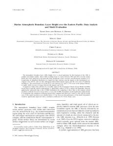
al., 2007; Sportisse, 2010). As air pollution becomes more severe due to economic development, particularly in developing countries (Wang et al., 2009), knowledge of h is important to the environmental science community and public. Furthermore, h is related to the warming rate that is caused by the enhanced greenhouse gases (Pielke et al., 2007). The average h is located in the middle of the entrainment layer where the strongest gradients of the vertical profiles of temperature, humidity and pollutants (Stull, 1988) are located. These profiles are provided by radio soundings and many remote sounding systems (Emeis et al., 2008). How498 ever, broad application of the remote sensing data has been hindered by the sharp extinction of the remote sensing 499 sig- Figure 1. Local solar time the radiosonde observation time (LST, in 00 UTC) at the Figure 1. Local solaroftime of the radiosonde observation time (LST, nal in high humidity conditions (e.g. cloud or fog) (Ferrero in 00:00 UTC) at the 79 stations over North America. 500 79 stations over the North America. et al., 2010; McGrath-Spangler and Denning, 2012). Many methods have been proposed to estimate h from the temperour study to local daytime (local solar time – LST). For most ature and atmospheric composition profiles (Seibert et al., stations in North America, the data observed at 00:00 UTC 2000; Basha and Ratnam, 2009; Seidel et al., 2010; Ferrero et correspond to the local daytime (Fig. 1). Because the mixing al., 2011; Seidel et al., 2012); however, inconsistencies exist layer is the convective boundary layer height in the daytime, among the methods (Seidel et al., 2010; von Engeln and Teixwe eliminated the radiosonde record with surface-based temeira, 2013). Seidel et al. (2010) compared h values that were perature inversion which may indicate the stable boundary derived from the existing methods using radiosonde data and layer. found substantial differences among the various methods. For example, the RH method systematically overestimates 2.2 Methods the h for the presence of clouds or introduces instrument errors (Seidel et al., 2010). In this paper, we attempt to ex2.2.1 Comparison of the existing methods to plain the nonconformity of various methods and propose a determine h method to combine all of the individual standards. The proposed method is applied to high temporal resolution (6 s) raSeveral approaches have been developed to estimate h from diosonde data available from the Stratospheric Processes and radiosonde data (Seidel et al., 2010; Basha and Ratnam, their Role in Climate Data Center (SPARC). 2009). Four widely accepted methods that are based on inThe following section provides a brief description of the dividual atmospheric variables were selected and compared data and our methodology. Section 3 presents the results of in this study. These methods are briefly summarised here. the method at 79 stations over North America during 1998– The potential temperature (θ ) profile, which indicates at2008, and the final section provides the conclusions and a mospheric static stability and significantly impacts pollutant discussion. diffusion, is the most common operational method to determine h. Considering the thickness of the entrainment zone, which is enhanced in a weak elevated inversion and intense 2 Data and methods wind shear conditions (Wang et al., 2008), we assume that 20 the level of the maximum gradient of the θ profile rather than 2.1 Data the inversion base is the mixing layer top. The mixing layer height derived from θ is referred to as “hθ ”, which represents High temporal resolution radiosonde data are obtained the transition from a convectively less stable region (below) from the Stratospheric Processes and their Role in Climate to a more stable region (above) (Garratt, 1994; Seidel et al., Data Center (SPARC) (http://www.sparc.sunysb.edu/html/ 2010). hres.html) for the period 1998 to 2008. The SPARC data Water vapour acts as a tracer of the atmospheric dispersion set consists of historical records at 79 stations over North state which contains and integrates the effects of physical America. This data set includes geopotential height, temperatmospheric forces (both thermal and mechanical) on subature, relative humidity and dew point temperature. These stance dispersion (Ferrero et al., 2010). The h can be estivariables are recorded at a 6 s interval, which approximately mated as the level of the minimum vertical gradient of rel−1 corresponds to a 30 m vertical resolution with a ∼ 5 m s ative humidity (hRH ) or specific humidity (hq ) with a sigvertical velocity of the balloon (Wang and Geller, 2003; Seinificant reduction in atmospheric moisture (Ao et al., 2008; del et al., 2012). Generally, measurements are obtained twice Seidel et al., 2010). daily at 00:00 and 12:00 Coordinated Universal Time (UTC). Because this study focuses on mixing layer height, we limit Atmos. Meas. Tech., 7, 1701–1709, 2014

www.atmos-meas-tech.net/7/1701/2014/

X. Y. Wang and K. C. Wang: Estimation of atmospheric mixing layer height from radiosonde data

1703

of hRH and hq , which are both estimated from water vapour variables, are not consistent (Fig. 2b), especially for a complicated humidity profile and a boundary layer that is not well mixed. 2.2.2

501 502 503 504 505 506 507 508 509

Reasons for discrepancies among different methods

In the case of a weak inversion or a non-perfectly mixed boundary layer, the entrainment zone is ambiguous; thus, various values of h can be measured (Martin et al., 1988; Seibert et al., 2000). Furthermore, the radiosonde humidity sensor can introduce systematic errors in clod and dry or cloudy conditions (Seibert et al., 2000; Moradi et al., 2013). Refractivity and specific humidity can be dominated by the water vapour pressure variations at lower altitudes, and they decrease rapidly with height (Ao et al., 2012; von Engeln and Teixeira, 2013). The breakpoint of the profile usually appears Figure 2. The profiles of relative (RH),temperature potential (temFigure 2. The profiles of relative humidityhumidity (RH), potential θ), specific at a low altitude, which leads to the shallow h values using perature (θ ), specific humidity (q), refractivity (N ) and the mixing these two methods. humidity (q), refractivity (N) and the mixing layer height (h) derived from these layer height (h) derived from these profiles. The y axis is the height Although some studies have suggested that coherence exprofiles. the height the ground level. h determined by individual ists among the various methods, most of the research was above The the Y-axis groundis level. Theabove h determined by individual standard (magenta dotteddotted line) line) and hand integrates of θθ, 0 which standard (magenta h0 which integratesthe theinformation information of , RH, q conducted in clear sky conditions (Kim et al., 2007; Ferrero RH, q and N (black solid line) are also shown. (a) Station #14898 at et al., 2011, 2010; McGrath-Spangler and Denning, 2013). and N (black solid line) are also shown. (a) Station #14898 at 00 UTC on 00:00 UTC on 13 August 2006, (b) station #14898 at 00:00 UTC on 13 in We suggest that the presence of clouds is an important factor ◦ ◦ 23 August (Station #14898: 44.5 onN,2388.1 W,2006. LST:(Station 18:06).#14898: August 2006, 2006. (b) Station #14898 at 00 UTC August that reduces the agreement of different methods. In the pres44.5°N, 88.1°W, local solar time: 18:06). ence of clouds, the humidity-based methods may identify the cloud top as the top of mixing layer due to the large negaAdditionally, atmospheric refractivity (N), which comtive humidity gradient there (von Engeln and Teixeira, 2013). bines the information of temperature and humidity (defined For example, the RH method combines the temperature and in Eq. (1)), is also used to determine the h. The height of the specific humidity to enlarge both gradients (von Engeln and minimum vertical gradient of refractivity (N) is referred to Teixeira, 2013). as “hN ”. The refractivity was calculated by (Xie et al., 2012; Generally, stratocumulus clouds are capped by an inverSeidel et al., 2010) sion (Stull, 1988), which can lead to the hθ value located at P e the cloud top. However, the humidity and temperature proN = (n − 1) × 106 = 77.6 + 3.73 × 105 2 , (1) T T files are not properly coincident near the cloud top (Dai, where N is refractivity, n is the refractive index, P is at- 21 2012). The maximum negative gradient of humidity occurs at mospheric pressure in hPa, T is atmospheric temperature in the top of the cloud, while the maximum gradient of potential Kelvin and e is water vapour pressure in hPa. temperature usually occurs in the middle of the entrainment To avoid mistaking free tropospheric features for the top layer above the cloud top (Moeng et al., 2005; Dai, 2012). of the mixing layer, if h was higher than 4000 m a.g.l., then Thus, for a thin entrainment layer, the hRH (hq ) and hθ are it was considered as missing data (Seidel et al., 2010). To faessentially the same. If the thickness of the transition cancilitate a comparison of the climatological h from stations at not be ignored because of a weak inversion and intense wind different elevations, the units for h are given as “metres above shear, then the hθ will be significantly higher than hRH and ground level”. To minimise the effect of extreme values, all hq (Moeng et al., 2005). Measurements have demonstrated of the profiles were smoothed using a 1–2–1 smoother: the that the air between the cloud top and the height of the maxsmoothed value at a given level was the sum of the values imum gradient of potential temperature in the entrainment at a lower level multiplied by 25 %, at the level of interest zone still includes turbulence and should be considered part multiplied by 50 %, and at a higher level multiplied by 25 %. of the mixing layer (Moeng et al., 2005; Lenschow et al., The h values that were derived from the profiles of po2000). In this case, hθ seems to be a reasonable definition of tential temperature, relative humidity, specific humidity and the mixing layer height. refractivity correlate well in 31.18 % of all of the cases (with Developing cumulus clouds display updrafts over a small a 50 m allowable error) (Fig. 2a), but were also observed to area. The cumulus clouds are surrounded by a combination of be substantially different in some cases (Fig. 2b). Generally, clear sky and passive cumulus over the remaining area (Stull, hθ and hRH are much higher than hq and hN . The values 1988; Zeng et al., 2004). The compensating subsidence over www.atmos-meas-tech.net/7/1701/2014/

Atmos. Meas. Tech., 7, 1701–1709, 2014

1704

X. Y. Wang and K. C. Wang: Estimation of atmospheric mixing layer height from radiosonde data

this area effectively produces a stable layer close to the cloud base (Zeng et al., 2004). Additionally, latent heat released in the cloud (Tjernström, 2007) can lead to a weak inversion in the cloud. The stable layer within the cloud can act as a turbulence barrier to the air pollution and inhibit turbulence under the stable layer. Nonetheless, clouds can also encourage pollutant dispersion and enhance mixing due to the cloud-venting (Cotton et al., 1995; Verzijlbergh et al., 2009). The vertical motion of pollutants mainly depends on the atmospheric stability in the cloud. In a stable stratification, air parcels are either neutrally or negatively buoyant, which reduces the buoyancy of the thermals beneath this layer through vertical mixing. In the case of a thick elevated stable stratification, the maximum vertical gradient of potential temperature regarded as h instead of cloud top, where a sharp reduction of moisture occurs (i.e. hRH or hq ). For deep convective clouds, updrafts in the cloud are strong enough to transport the air in the mixing layer to the upper free atmosphere. The h should be defined as the cloud base to avoid mistaking the top of the troposphere as the top of the mixing layer (Stull, 1988). In our study, the mixing layer is limited to 4000 m, which may exclude cases of deep convective clouds in the boundary layer. 2.2.3

A reliable method to produce consistent estimates of mixing layer height (hcon )

Although all four of the variables can introduce uncertainties into the h estimation, the temperature and humidity factors are the most important for producing a superior h estimation: the temperature quantifies the inversion and the water vapour describes the mixing capability. In this section, we propose an integrated method that contains the information of temperature and moisture, and provides a reasonable definition of a cloud-capped mixing layer height. For a non-perfectly mixed boundary layer, the method may not simultaneously satisfy the criteria that all four individual variables have the highest vertical gradients at the same level. Instead, we identify the height where the criteria are best met and label it h0 . In other words, all of the variables exhibit sharp variations at the selected height (h0 ), but not necessarily the sharpest variations of the entire profiles. For stratocumulus and stratus capped boundary layers, inversions are located near the cloud top, whereas for some cumulus, the stable layer usually occurs near the cloud base (Zeng et al., 2004). The level with the greatest potential temperature gradient in the stable layer near the cloud is hcon (see Sect. 2.2.1). Considering that the average distance between the cloud top and the level of the largest potential temperature gradient in the entrainment zone is approximately 20 m (Moeng et al., 2005), we scan 90 m (∼ 3 levels with the 30 m vertical resolution radiosonde data) upward from the cloud top to identify any inversions. Likewise, we search three levels downward and upward of the cloud to ensure the existence of a stable layer. If a stable layer cannot be identified Atmos. Meas. Tech., 7, 1701–1709, 2014

near the cloud, then the h0 is set as hcon ; thus, cloud is assumed to enhance the mixing. Clouds are derived from the radiosonde data set by referencing the relative humidity to a specific threshold, based on the method proposed by Wang and Poore (Poore et al., 1995). The method was later modified by Zhang (Zhang et al., 2010) and validated by independent observations (Zhang et al., 2013). Following the above qualitative guidelines, an objective approach is proposed based on our radiosonde data. 1. Identify the height (h0 ) that best meets the four individual criteria: a. Smooth the gradient profiles of θ, RH, q and N by 1–2–1 smoother. b. Locate the altitudes of the 10 smallest gradients (or largest for θ) of the four variables. All 10 altitudes are considered to meet the criterion of the mixing layer top and are likely to be the h. c. Starting with the altitudes of the smallest gradients (or largest for θ ), identify the first altitude where at least three of the four variables meet the criteria of h simultaneously. The altitude meeting these criteria is set as h0 . The allowable error is 50 m. If all altitudes do not meet the criteria until the 10th smallest gradient, then the mixing layer height for the specific record is missing. 2. Derive the location of the cloud (Zhang et al., 2010): a. Transform the RH with respect to ice instead of liquid water for all of the levels with temperatures below 0 ◦ C. b. Derive the boundary of the moist layer. The base of the moist layer is defined as the level where the RH exceeds the min-RH corresponding to this level. Likewise, the top of the moist layer is determined as the level where the RH decreases to the minRH corresponding to the level or where the top of the profile is reached. Any moist layer with a base lower than 120 m was discarded. The min-RH value is specified in Table 1. c. The moist layer is classified as a cloud layer if the maximum RH within this layer is greater than the corresponding max-RH at the base of the moist layer. Two contiguous layers are considered a onelayer cloud if the distance between the two layers is less than 300 m or if the minimum RH over the distance is larger than the maximum inter-RH value within this distance. The max-RH, inter-RH values are specified in Table 1.

www.atmos-meas-tech.net/7/1701/2014/

X. Y. Wang and K. C. Wang: Estimation of atmospheric mixing layer height from radiosonde data

1705

Table 1. Summary of height-resolving RH thresholds for cloud detection. Altitude range

min-RH (%)

max-RH (%)

inter-RH (%)

0–2 km 2–6 km 6–12 km > 12 km

92–90 90–88 88–75 75

95–93 93–90 90–80 80

84–82 80–78 78–70 70

3. Determine a consistent mixing layer height (hcon ): a. If the h0 is lower than the base of the lowest cloud or identified in clear sky conditions, then the hcon equals h0 . b. If the h0 is higher than the base of the lowest cloud, then scan from the lower three levels of the cloud base to the upper three levels of the cloud top to identify the first stable layer that is deeper than 100 m. Set the level of the sharpest inversion in the 510 stable layer as hcon . If a stable layer does not exist within the cloud, then the hcon equals h0 . 511

Figure 3. The profiles of potential temperature (θ), relative humidity (RH) humid(red line is Figure 3. The profiles of potential temperature (θ), relative

512 layer

ityRH(RH) (thetored is black the RH with respect the liquid the respected the profile water and line indicates the RHto respected to icewawhen

Figure 3 displays three cases in which the boundary clouds affect the development of turbulence. When an inver513 sion caps the top of the cloud (Fig. 3a) or is located near the 514 cloud base (Fig. 3b), then the level of the sharpest inversion 515 is assigned as the mixing layer height. In this case, the inver516 sion near the cloud inhibits the diffusion of pollutants. In the 517 scenario depicted in Fig. 3c, a stable layer is not identified, 518 the cloud accelerates the diffusion and the hcon is considered as the h0 .

ter and the black profile indicates the RH with respect to ice when

the temperature below 0°C), specific humidity (q), refractivity (N) and the mixing the temperature is below 0 ◦ C), specific humidity (q), refractivity layer Themixing Y-axis is layer the height above the level. derivedabove from the (N)heights. and the heights. Theground y axis is Cloud the height

ground level. Cloud derived from the RH with to ice (35.2°N, is loRH respected to ice is located at the shadow region. (a) respect Station #03948 cated in the shadow region. (a) Station #03948 (35.2◦ N, 97.4◦ W) 97.4°W) at 00 UTC (17:30 LST) on 22 May 2001; (b) Station #14898 (44.5°N, at 00:00 UTC (17:30 LST) on 22 May 2001; (b) station #14898

◦ W) 88.1°W) UTC (18:06 LST) on 25 August Station #12850 2006; (24.5°N, (44.5◦ atN,0088.1 at 00:00 UTC (18:062006; LST)(c)on 25 August ◦ ◦ (c) station (24.5 81.8 at 00:00 UTC (18:30 LST) on 81.8°W) at 00 #12850 UTC (18:30 LST) N, on 10 JulyW) 2000.

10 July 2000. 100

3

Results

θ

(a) 80

3.1

Statistical properties of the mixing layer height (hcon ) estimates

The statistical results of the h0 location within the top 10 gradients of each individual variable are presented in Fig. 4. In most cases, the h0 corresponds to the highest gradients, which means that the h0 is consistent with that determined by the individual standards of θ, RH, q and N in most cases. The potential temperature has the highest missing value; thus, only three standards (RH, q and N) typically meet the criteria. The results also indicate that the h determined by the θ and RH methods significantly deviate from the h0 . The h0 has a high coherence with the hq and hN (79 % and 85 %, www.atmos-meas-tech.net/7/1701/2014/

q

N 22

10 (b)

Percentage(%)

Section 2 describes a method to integrate existing standards to produce a consistent estimate of mixing layer height. The statistical properties of the estimate and a comparison with the existing methods are discussed in this section. Additionally, the North American mixing layer height climatology is presented.

RH

60

5

40

0

2nd 3rd 4th 5th 6th 7th 8th 9th 10th

20

0

1st

2nd

3rd 4th 5th 6th 7th 8th 9th Location of h0 in the Top Ten Gradient List

10th Missing

Figure 4. The statistical result of the consistency between h0 (h0 which integrates the information of θ , RH, q and N) and the four existing methods at the 79 North America stations. Percentage in “1st” means the h0 coincides with the existing method. The missing value means the case of the h0 did not exist in the top 10 gradient lists for the specific variable and the h0 is determined by the other three standards. The subgraph (b) shows a close-up view of the 2nd to 10th in (a).

Atmos. Meas. Tech., 7, 1701–1709, 2014

1706

X. Y. Wang and K. C. Wang: Estimation of atmospheric mixing layer height from radiosonde data

526 527

Figure 5. The frequency histogram of the effect of cloud on pollutants diffusion. The

528

“clear indicates The there “clear is no cloud the boundary boundary tantssky” diffusion. sky”inindicates thatlayer, thereotherwise, is no cloud in

529

the isboundary layer; otherwise, means the boundary layer isturbulence cloud-taped. layer cloud-taped; “cloud-enhance” clouds stimulate in the

530

The “cloud-enhance” means thatindicates clouds the stimulate cloud-capped conditions; “cloud-inhibit” case thatturbulence the inversionininthe the

531

cloud suppresses turbulence in the cloud-capped conditions. The stations are sorted by

532

Figure 5. Frequency histogram of the effect of cloud on pollu-

cloud-capped conditions. The “cloud-inhibit” indicates the case that the inversion in the cloud suppresses turbulence in the cloud-capped theconditions. value of clearThe sky percentage. stations are sorted by the value of clear sky 533 percentage. 534 Figure 6. Figure The comparison of the hconhcon withwith hθ h(blue), hRH (red), hq 6. Comparison of climatological the climatological θ (blue), hRH (red), hq (green), hN (brown) and h0 (black) for the period 535h , h(green), hN (brown) and h0 (black) for the period of 1998 to 2008. Table 2. A summary of the comparison of the hcon with θ RH , 1998–2008. hq , hN and h0 , including correlation coefficient, bias and standard deviation. hcon is the final consistent estimate of h which include the information of temperature, water vapour and cloud; hθ , hRH , if the monthly values are available for more than 6 months hq , hN are the h derived from the individual standard of potential during a year. The climatological h values for 57 of the 79 temperature (θ ), relative humidity (RH), specific humidity (q) and stations that meet these requirements are shown in Fig. 6 atmospheric refractivity (N ) respectively; h0 indicates the h inteand summarised in Table 2. The averages of the hcon and h0 grating the information of θ, RH, q and N which is a transition to are 1675 m and 1713 m, respectively; thus, the h decreases the hcon . hcon

Method Correlation coefficient Bias (m) Standard deviation (m)

hθ

hRH

hq

hN

h0

0.86 506.2 161.5

0.90 522.9 131.1

0.96 116.2 71.4

0.97 −22.9 74.8

0.98 37.6 25.1 24

respectively) and a relatively low coherence with the hθ and hRH (44 % and 68 %, respectively). Figure 5 displays the percentage of the h0 values that are influenced by clouds at the 79 stations: 72.3 % of the mixing layer has clear sky conditions (no clouds in the lowest 4000 m above the surface) and 27.7 % of the mixing layer is cloud-capped. In the cloud-capped scenarios, the clouds stimulate turbulence for approximate one-third of the cloudy cases. For the other two-thirds of the cases, inversions near the clouds suppress turbulence; therefore, the level of the sharpest inversion is the mixing layer height. However, the N method never defines cloud base as h because of the higher refractivity in clouds than beneath clear air. 3.2

Comparison of hcon with other methods

To reduce the impact of missing data, we calculated the monthly h only if the daily h is available for more than 15 days during a month. The annual h is only calculated Atmos. Meas. Tech., 7, 1701–1709, 2014

by 38 m when considering the cloud impacts on turbulence. The values of the hRH and hθ have much higher mean values (2199 m and 2182 m, respectively) and lower coherence with the hcon . The climatologies of the hq and hN are relatively lower: 1792 m and 1653 m, respectively. The value of the hN has the best agreement with hcon , which may be due to the information of temperature and water vapour contained in the refractivity concurrently. However, the contribution of water vapour to the refractivity may be higher than that of temperature in the lower troposphere (Basha and Ratnam, 2009); the N method cannot account for the effect of clouds. Furthermore, the temperature variable can derive the vertical structure of the cloud. Therefore, the temperature and moisture information provided by the radiosonde can be a vital resource to estimate the mixing layer height. 3.3

Climatology of mixing layer height over North America

Figure 7 displays the multi-year average of the hcon pattern over North America. A strong east–west h gradient where the higher h over the western states is consistent with the spatial distribution of the h derived from the Cloud-Aerosol Lidar with Orthogonal Polarization (CALIOP) data set of the CALIPSO satellite (McGrath-Spangler and Denning, 2012, 2013). The climatological h over the Midwest US is generally greater than 1800 m, whereas the values are usually less than 1400 m over Alaska and the US West Coast due www.atmos-meas-tech.net/7/1701/2014/

25

X. Y. Wang and K. C. Wang: Estimation of atmospheric mixing layer height from radiosonde data

536 537 538 539

1707

h at 57 stations over North America, derived from the radiosonde data of SPARC during 1998–2008, is 1675 ± 303 m. The analysis of the climatological h over North America revealed a noteworthy feature: a strong east–west gradient of h exists, where higher values (generally greater than 1800 m) occur over the Midwest US due to the high topography and low soil moisture, whereas lower h values (usually less than 1400 m) occur over Alaska and the US West Coast, associated with the high latitude and cold upwelling water, respectively. A qualitative comparison of our method with the mixing layer height derived from space-borne lidar was conducted. Figure 7. Pattern of climatological hcon overhNorth America the period Figure 7. Pattern of climatological Northduring America duringof 1998However, a detailed validation of the new method is difficult con over the period 1998–2008 (unit: m). The 57 stations shown here are to 2008 (unit: meter). All the 57 stations showed here are the stations whothe meet thebecause the observations are available at substantially difstations which meet the long-term average criteria mentioned at the ferent local solar time, and the mixing layer height has an long-term average criteria3.1. mentioned at the beginning of Sect 3.1. beginning of Sect. important diurnal cycle. Future work should consider the diurnal cycle of h from model simulations. to the high latitude and cold upwelling water, respectively. Frequent precipitation and high moisture may cause the relatively shallower h over the Mississippi River because a large fraction of the net radiation in this region is used to evaporate water, leaving less energy to enhance the h (McGrathSpangler and Denning, 2012). A possible explanation for the deep h along the semiarid Rocky Mountains in the southwestern US is that the low soil moisture characteristic of the high elevations provides enough sensible heat flux to extend the h. However, because the region spans several time zones, the spatial variations observed at a fixed time may be affected by temporal variations. The mixing layer begins to develop after sunrise due to the increased turbulent fluxes associated with surface-absorbed solar radiation and heating (Medeiros et al., 2005; Liu and Liang, 2010). The value of h reaches its maximum during the late afternoon over land (Liu and Liang, 2010; Bianco et al., 2011; Svensson et al., 2011). Comparing Fig. 7 with Fig. 1, the deep mixing layer in the western US is likely associated with the afternoon convection. 4

Conclusions and discussion

To address the problem of the disagreement of h values that are derived from existing methods and the effect of stable stratification in clouds on the diffusion of pollutants, we proposed a method to integrate the information of temperature, humidity and cloud effects to determine a consistent estimate of the h. The h that is derived from the proposed method better agrees with those values that are derived from the N method (N includes information of both temperature and water vapour). Our results also agree well with observations from satellite lidar. The proposed method determines the h by accounting for the boundary layer clouds. The method that is used to determine clouds was recently validated by independent observations (Zhang et al., 2013). The climatological www.atmos-meas-tech.net/7/1701/2014/

Acknowledgements. This study is funded by the National Basic Research Programme of China (2012CB955302) and the National Natural Science Foundation of China (41175126 and 91337111). The radiosonde data used in this study were provided by Stratospheric Processes and their Role in Climate Data (http://www.sparc.sunysb.edu/html/hres.html). Edited by: L. Bianco

References Ao, C., Chan, T., Iijima, B., Li, J., Mannucci, A., Teixeira, J., Tian, B., and Waliser, D.: Planetary boundary layer information from GPS radio occultation measurements, GRAS SAF Workshop on Applications of GPSRO Measurements, 2008, 123–131, 2008. Ao, C. O., Waliser, D. E., Chan, S. K., Li, J. L., Tian, B., Xie, F., and Mannucci, A. J.: Planetary boundary layer heights from GPS radio occultation refractivity and humidity profiles, J. Geophys. Res.-Atoms., 117, D16117, doi:10.1029/2012JD017598, 2012. 26Basha, G. and Ratnam, M. V.: Identification of atmospheric boundary layer height over a tropical station using high–resolution radiosonde refractivity profiles: Comparison with GPS radio occultation measurements, J. Geophys. Res.-Atmos., 114, D16101, doi:10.1029/2008JD011692, 2009. Bianco, L., Djalalova, I. V., King, C. W., and Wilczak, J. M.: Diurnal Evolution and Annual Variability of Boundary-Layer Height and Its Correlation to Other Meteorological Variables in California’s Central Valley, Bound.-Lay. Meteorol., 140, 491–511, doi:10.1007/s10546-011-9622-4, 2011. Cotton, W. R., Alexander, G. D., Hertenstein, R., Walko, R. L., McAnelly, R. L., and Nicholls, M.: Cloud venting – A review and some new global annual estimates, Earth-Sci. Rev., 39, 169– 206, 1995. Dai, C. Y.: Properties of the entrainment zone atop the atmospheric boundary layer and determination of the boundary layer height, Ph.D, Institute of Atmospheric Physics, Chinese Academy of Sciences, China, 129 pp., 2012.

Atmos. Meas. Tech., 7, 1701–1709, 2014

1708

X. Y. Wang and K. C. Wang: Estimation of atmospheric mixing layer height from radiosonde data

Emeis, S., Schaefer, K., and Muenkel, C.: Surface-based remote sensing of the mixing-layer height-a review, Meteorol. Z., 17, 621–630, doi:10.1127/0941-2948/2008/0312, 2008. Ferrero, L., Perrone, M. G., Petraccone, S., Sangiorgi, G., Ferrini, B. S., Lo Porto, C., Lazzati, Z., Cocchi, D., Bruno, F., Greco, F., Riccio, A., and Bolzacchini, E.: Vertically-resolved particle size distribution within and above the mixing layer over the Milan metropolitan area, Atmos. Chem. Phys., 10, 3915–3932, doi:10.5194/acp-10-3915-2010, 2010. Ferrero, L., Riccio, A., Perrone, M., Sangiorgi, G., Ferrini, B., and Bolzacchini, E.: Mixing height determination by tethered balloon-based particle soundings and modeling simulations, Atmos. Res., 102, 145–156, 10.1016/j.atmosres.2011.06.016, 2011. Garratt, J. R.: The atmospheric boundary layer, Cambridge university press, 1994. Kim, S.-W., Yoon, S.-C., Won, J.-G., and Choi, S.-C.: Ground-based remote sensing measurements of aerosol and ozone in an urban area: A case study of mixing height evolution and its effect on ground-level ozone concentrations, Atmos. Environ, 41, 7069– 7081, doi:10.1016/j.atmosenv.2007.04.063, 2007. Lenschow, D. H., Zhou, M., Zeng, X., Chen, L., and Xu, X.: Measurements of fine-scale structure at the top of marine stratocumulus, Bound-Lay. Meteorol., 97, 331–357, doi:10.1023/A:1002780019748, 2000. Liu, S. and Liang, X.-Z.: Observed Diurnal Cycle Climatology of Planetary Boundary Layer Height, J. Climate, 23, 5790–5809, doi:10.1175/2010jcli3552.1, 2010. Martin, C. L., Fitzjarrald, D., Garstang, M., Oliveira, A. P., Greco, S., and Browell, E.: Structure and growth of the mixing layer over the Amazonian rain forest, J. Geophys. Res-Atmos., 93, 1361– 1375, doi:10.1029/JD093iD02p01361, 1988. McGrath-Spangler, E. L. and Denning, A. S.: Estimates of North American summertime planetary boundary layer depths derived from space-borne lidar, J. Geophys. Res-Atmos., 117, D15101, doi:10.1029/2012JD017615, 2012. McGrath-Spangler, E. L. and Denning, A. S.: Global seasonal variations of midday planetary boundary layer depth from CALIPSO space-borne LIDAR, J. Geophys. Res-Atmos., 118, 1226–1233, doi:10.1002/jgrd.50198, 2013. Medeiros, B., Hall, A., and Stevens, B.: What controls the mean depth of the PBL?, J. Climate, 18, 3157–3172, doi:10.1175/jcli3417.1, 2005. Menut, L., Flamant, C., Pelon, J., and Flamant, P. H.: Urban boundary-layer height determination from lidar measurements over the Paris area, Appl. Optics, 38, 945–954, doi:10.1364/AO.38.000945, 1999. Moeng, C., Stevens, B., and Sullivan, P.: Where is the interface of the stratocumulus-topped PBL?, J. Atmos. Sci., 62, 2626–2631, doi:10.1175/JAS3470.1, 2005. Moradi, I., Soden, B., Ferraro, R., Arkin, P., and Vömel, H.: Assessing the quality of humidity measurements from global operational radiosonde sensors, J. Geophys. Res-Atmos., 118, 8040– 8053, doi:10.1002/jgrd.50589, 2013. Pielke, R. A., Davey, C. A., Niyogi, D., Fall, S., Steinweg-Woods, J., Hubbard, K., Lin, X., Cai, M., Lim, Y. K., and Li, H.: Unresolved issues with the assessment of multidecadal global land surface temperature trends, J. Geophys. Res., 112, D16113, doi:10.1029/2006JD008229, 2007.

Atmos. Meas. Tech., 7, 1701–1709, 2014

Poore, K. D., Junhong, W., and Rossow, W. B.: Cloud layer thicknesses from a combination of surface and upper-air observations, J. Climate, 8, 550–568, 1995. Russell, P. B., Uthe, E. E., Ludwig, F. L., and Shaw, N. A.: A comparison of atmospheric structure as observed with monostatic acoustic sounder and lidar techniques, J. Geophys. Res., 79, 5555–5566, doi:10.1029/JC079i036p05555, 1974. Seibert, P., Beyrich, F., Gryning, S.-E., Joffre, S., Rasmussen, A., and Tercier, P.: Review and intercomparison of operational methods for the determination of the mixing height, Atmos. Environ, 34, 1001–1027, doi:10.s1352-2310(99)00349-0, 2000. Seidel, D. J., Ao, C. O., and Li, K.: Estimating climatological planetary boundary layer heights from radiosonde observations: Comparison of methods and uncertainty analysis, J. Geophys. Res., 115, D16113, doi:10.1029/2009JD013680, 2010. Seidel, D. J., Zhang, Y., Beljaars, A., Golaz, J. C., Jacobson, A. R., and Medeiros, B.: Climatology of the planetary boundary layer over the continental United States and Europe, J. Geophys. Res., 117, D17106, doi:10.1029/2012JD018143, 2012. Sportisse, B.: Fundamentals in air pollution: from processes to modelling, Atmospheric Boundary Layer, Springer, 93–132, 2010. Stull, R. B.: An introduction to boundary layer meteorology, Kluwer academic publishers, 665 pp., 1988. Svensson, G., Holtslag, A. A. M., Kumar, V., Mauritsen, T., Steeneveld, G. J., Angevine, W. M., Bazile, E., Beljaars, A., de Bruijn, E. I. F., Cheng, A., Conangla, L., Cuxart, J., Ek, M., Falk, M. J., Freedman, F., Kitagawa, H., Larson, V. E., Lock, A., Mailhot, J., Masson, V., Park, S., Pleim, J., Soderberg, S., Weng, W., and Zampieri, M.: Evaluation of the Diurnal Cycle in the Atmospheric Boundary Layer Over Land as Represented by a Variety of Single-Column Models: The Second GABLS Experiment, Bound.-Lay. Meteorol., 140, 177–206, doi:10.1007/s10546-0119611-7, 2011. Tjernström, M.: Is There a Diurnal Cycle in the Summer CloudCapped Arctic Boundary Layer?, J. Atmos. Sci., 64, 3970–3986, doi:10.1175/2007JAS2257.1, 2007. Verzijlbergh, R. A., Jonker, H. J. J., Heus, T., and Vilà-Guerau de Arellano, J.: Turbulent dispersion in cloud-topped boundary layers, Atmos. Chem. Phys., 9, 1289–1302, doi:10.5194/acp-91289-2009, 2009. von Engeln, A. and Teixeira, J.: A Planetary Boundary Layer Height Climatology Derived from ECMWF Reanalysis Data, J. Climate, 26, 6575–6590, doi:10.1175/JCLI-D-12-00385.1, 2013. Wang, K. C. and Dickinson, R. E.: Global atmospheric downward longwave radiation at the surface from ground-observations, satellite retrievals and reanalyses, Rev. Geophys., 51, 150–185, doi:10.1002/rog.20009, 2013. Wang, K. C., Wang, P., Li, Z., Cribb, M., and Sparrow, M.: A simple method to estimate actual evapotranspiration from a combination of net radiation, vegetation index, and temperature, J. Geophys. Res., 112, D15101, doi:10.1029/2006JD008351, 2007. Wang, K. C., Dickinson, R. E., and Shunlin, L.: Clear sky visibility has decreased over land globally from 1973 to 2007, Science, 323, 1468–1470, doi:10.1126/science.1167549, 2009. Wang, K. C., Dickinson, R. E., Wild, M., and Liang, S.: Atmospheric impacts on climatic variability of surface incident solar radiation, Atmos. Chem. Phys., 12, 9581–9592, doi:10.5194/acp12-9581-2012, 2012.

www.atmos-meas-tech.net/7/1701/2014/

X. Y. Wang and K. C. Wang: Estimation of atmospheric mixing layer height from radiosonde data Wang, L. and Geller, M. A.: Morphology of gravity-wave energy as observed from 4 years (1998–2001) of high vertical resolution US radiosonde data, J. Geophys. Res., 108, 4489, doi:10.1029/2002JD002786, 2003. Wang, S., Golaz, J. C., and Wang, Q.: Effect of intense wind shear across the inversion on stratocumulus clouds, Geophys. Res. Lett., 35, L15814, doi:10.1029/2008GL033865, 2008. Xie, F., Wu, D. L., Ao, C. O., Mannucci, A. J., and Kursinski, E. R.: Advances and limitations of atmospheric boundary layer observations with GPS occultation over southeast Pacific Ocean, Atmos. Chem. Phys., 12, 903–918, doi:10.5194/acp-12-903-2012, 2012.

www.atmos-meas-tech.net/7/1701/2014/

1709

Zeng, X., Brunke, M. A., Zhou, M., Fairall, C., Bond, N. A., and Lenschow, D. H.: Marine atmospheric boundary layer height over the eastern Pacific: Data analysis and model evaluation, J. Climate, 17, 4159–4170, doi:10.1175/JCLI3190.1, 2004. Zhang, J., Chen, H., Li, Z., Fan, X., Peng, L., Yu, Y., and Cribb, M.: Analysis of cloud layer structure in Shouxian, China using RS92 radiosonde aided by 95 GHz cloud radar, J. Geophys. Res., 115, D00K30, doi:10.1029/2010JD014030, 2010. Zhang, J., Li, Z., Chen, H., and Cribb, M.: Validation of a radiosonde based cloud layer detection method against a ground– remote sensing method at multiple ARM sites, J. Geophys. ResAtmos., 118, 846–858, doi:10.1029/2012JD018515, 2013.

Atmos. Meas. Tech., 7, 1701–1709, 2014