1129
Estimation of biophysical characteristics for highly variable mixed-conifer stands using small-footprint lidar Jennifer L. Rooker Jensen, Karen S. Humes, Tamara Conner, Christopher J. Williams, and John DeGroot
Abstract: Although lidar data are widely available from commercial contractors, operational use in North America is still limited by both cost and the uncertainty of large-scale application and associated model accuracy issues. We analyzed whether small-footprint lidar data obtained from five noncontiguous geographic areas with varying species and structural composition, silvicultural practices, and topography could be used in a single regression model to produce accurate estimates of commonly obtained forest inventory attributes on the Nez Perce Reservation in northern Idaho, USA. Lidarderived height metrics were used as predictor variables in a best-subset multiple linear regression procedure to determine whether a suite of stand inventory variables could be accurately estimated. Empirical relationships between lidar-derived height metrics and field-measured dependent variables were developed with training data and acceptable models validated with an independent subset. Models were then fit with all data, resulting in coefficients of determination and root mean square errors (respectively) for seven biophysical characteristics, including maximum canopy height (0.91, 3.03 m), mean canopy height (0.79, 2.64 m), quadratic mean DBH (0.61, 6.31 cm), total basal area (0.91, 2.99 m2/ha), ellipsoidal crown closure (0.80, 0.08%), total wood volume (0.93, 24.65 m3/ha), and large saw-wood volume (0.75, 28.76 m3/ha). Although these regression models cannot be generalized to other sites without additional testing, the results obtained in this study suggest that for these types of mixed-conifer forests, some biophysical characteristics can be adequately estimated using a single regression model over stands with highly variable structural characteristics and topography. Résumé : Même si les données lidar sont largement disponibles auprès de compagnies commerciales, leur utilisation opérationnelle en Amérique du Nord demeure encore limitée tant à cause des coûts que de l’incertitude pour une application à grande échelle et des problèmes d’exactitude associés à la modélisation. Les auteurs ont analysé si les données lidar à petite empreinte au sol obtenues pour cinq régions géographiques non contiguës qui variaient en compositions spécifique et structurale, pratiques sylvicoles et topographie pouvaient être utilisées dans un modèle de régression unique pour produire des estimations exactes des attributs communément obtenus lors d’inventaires forestiers dans la réserve de Nez Perce située dans le nord de l’Idaho, aux É.-U. Les mesures de hauteur dérivées du lidar ont été utilisées comme variables prédictives dans une procédure de régression linéaire multiple du meilleur sous-ensemble pour déterminer si un ensemble de variables d’inventaire à l’échelle du peuplement pouvaient être estimées avec exactitude. Les relations empiriques entre les mesures de hauteur dérivées du lidar et les variables dépendantes mesurées sur le terrain ont été développées avec des données d’entraînement et des modèles acceptables validés avec un sous-ensemble indépendant. Les modèles ont ensuite été dérivés avec toutes les données, ce qui a produit des coefficients de détermination et des erreurs quadratiques moyennes (respectivement) pour sept caractéristiques biophysiques incluant : la hauteur maximale du couvert (0,91, 3,03 m), la hauteur moyenne du couvert (0,79, 2,64 m), le DHP moyen quadratique, (0,61, 6,31 m), la surface terrière totale (0,91, 2,99 m2/ha), la fermeture ellipsoïdale du couvert (0,80, 0,08 %), le volume total de bois (0,93, 24,65 m3/ha) et le volume de gros bois de sciage (0,75, 28,76 m3/ha). Même si ces modèles de régression ne peuvent pas être généralisés à d’autres sites sans tests additionnels, les résultats obtenus dans cette étude indiquent que, pour ces types de forêts mélangées résineuses, quelques caractéristiques biophysiques peuvent être estimées adéquatement par l’utilisation d’un modèle de régression unique pour des peuplements dont les caractéristiques structurales et la topographie sont très variables. [Traduit par la Rédaction]
Rooker Jensen et al.
1138
Received 24 June 2005. Accepted 14 December 2005. Published on the NRC Research Press Web site at http://cjfr.nrc.ca on 13 April 2006. J.L. Rooker Jensen1 and K.S. Humes. Department of Geography, University of Idaho, 375 South Line Street, McClure Hall 203, Moscow, ID 83844-3021, USA. T. Conner. USDA Forest Service, Ketchikan-Misty Fjords Ranger District, R10-Ketchikan Misty Fjords Road, 3031 Tongass Avenue, Ketchikan, AK 99901, USA. C.J. Williams. Department of Statistics, College of Science, University of Idaho, Brink Hall Room 415A, PO Box 441104, Moscow, ID 83844-1104, USA. J. DeGroot. Nez Perce Tribal Forestry, P.O. Box 365, Lapwai, ID 83540, USA. 1
Corresponding author (e-mail:
[email protected]).
Can. J. For. Res. 36: 1129–1138 (2006)
doi:10.1139/X06-007
© 2006 NRC Canada
1130
Introduction An accurate evaluation of any forest stand is central to forest and wildlife land management, as it assists in determining forest inventory, wildlife habitat requirements, and disease and pest hazards. An important tool aiding land managers with this task is the implementation and analysis of remotely sensed data. Numerous studies throughout the past several decades have described, with increasingly positive results, the ability of single- and multiple-return lidarderived height metrics to estimate canopy height and other specific forest characteristics such as volume, basal area, and stem density (Aldred and Bonner 1985; Maclean and Krabill 1986; Nelson et al. 1988; Means et al. 2000; Lefsky et al. 2001; Naesset and Bjerknes 2001; Naesset 2002; Holmgren et al. 2003; Lim et al. 2003a; Omasa et al. 2003; Holmgren 2004; Maltamo et al. 2004; Suarez et al. 2005). Lidar, which stands for light detection and ranging, is an active sensor that measures the time between laser pulse emission over a target and subsequent return to the sensor. There are two distinct forms of lidar remote sensing: waveform (large footprint) and discrete return (small footprint). The differences between waveform and discrete-return lidar involve the area actively sensed by the laser pulse and the spatially explicit information returned to the sensor. Waveform lidar sensors typically have a footprint, or horizontal scan area, 8–70 m in diameter (Lim et al. 2003b) and measure the temporal change in intensity of the returned energy, resulting in a documentation of the height distribution of the specified target (Dubayah and Drake 2000). Discrete-return lidar sensors operate by rapidly emitting a laser pulse toward a target (e.g., a forest stand) and recording the time, location, and quantity of the reflected energy. The sensor is mounted on an aircraft in conjunction with a highly accurate GPS and an inertial measurement unit (IMU), which allows correction in data processing caused by the attitude (pitch, roll, and yaw) of the aircraft. The aircraft is then flown over the area of interest, and the lidar sensor emits a series of high-frequency near-infrared (900– 1064 nm) pulses over the region. As the pulses are reflected from a target and the energy returns to the sensor, a record of the geographic coordinates and time from leaving the sensor and returning to the aircraft is generated. Early systems only recorded one returned pulse, but most current multireturn sensors record multiple returns from a single laser pulse (Lefsky et al. 2002). For a more detailed description of laser pulse interactions with forest canopies, the reader is referred to Lim et al. (2003b). Two forest measurements most commonly estimated with lidar are maximum height and mean canopy height (Naesset 1997; Naesset and Okland 2002). This is likely due to the close relationship between those surface characteristics and the quantities directly measured by a laser scanner (Maclean and Krabill 1986; Magnussen and Boudewyn 1998; Lim et al. 2003b). Several studies have also been developed with the goal of predicting vertical canopy structure (Ritchie et al. 1993; Zimble et al. 2003). Canopy structure, as defined in this paper, is the quantification of dimensional measurements of tree height and associated characteristics. Such characteristics are significant, as they provide knowledge of size-class distribution and total biomass for a given region
Can. J. For. Res. Vol. 36, 2006
(Lefsky et al. 1999). Measurement and inventory of such variables can aid in the characterization of a range of land management decisions, such as defining existing or potential wildlife habitat and quantifying carbon storage and source potential. Although recent research continues to affirm the usefulness of lidar data for deriving canopy-related forest characteristics, most studies demonstrating the effectiveness of small- and large-footprint lidar-derived height metrics for estimating biophysical characteristics have been limited to rather homogeneous geographic areas dominated by single or codominant species in relatively even-aged forest stands and uniform management scenarios. Few studies have been published that use lidar-derived height metrics to estimate stand characteristics in mixed-conifer forests with highly variable stand structure, species composition, and topographic conditions. Parker and Evans (2004) documented the utility of lidar-derived height metrics to model volume and biomass within stands composed of mixed-conifer species. Zimble et al. (2003) examined the relationship between lidar height metrics and vertical stand structural classifications for a mixture of six coniferous species. Naesset et al. (2005) developed empirical models to estimate stand characteristics from two separate inventories of young and mature forest stands of varying site quality and topography. However, in addition to species composition and topography, variation in silvicultural practices across a region can also factor into the ability of height metrics to predict biocharacteristics, in that tree size and density can be highly spatially variable in actively managed areas. This subject was taken into consideration by Andersen et al. (2005), who distributed sample plots throughout their study site, which was located in an ongoing experimental silvicultural trial with stands of varying age and density. Lefsky et al. (2005) applied lidar data from a largefootprint system to predict stand structural characteristics based on a composite sample of wide-ranging species, climatic, and topographic characteristics obtained from five distinct geographic locales in the Pacific Northwest. We present an analogous study, albeit with a smaller spatial extent, to estimate heterogeneous stand structural characteristics using data obtained from a small-footprint lidar sensor over a set of separate geographic study units. Lidar data are widely available from commercial contractors; however, operational use in North America is still limited by both economic cost and scientific uncertainty. Nelson et al. (2003) cite data acquisition and processing costs as well as assessment of large-scale application and associated accuracy issues as primary concerns. Although alternate statistical methods such as geostatistical analysis (Hudak et al. 2002) and imputation (Moeur and Stage 1995; Ohman and Gregory 2002; Maltamo et al. 2003) have been applied to predict forest biocharacteristics, regression analysis has proved to be a consistent and reliable statistical method for quantifying the relationship between lidar-derived height metrics and physical forest inventory variables. However, the range of stand and topographic conditions over which a single regression model can adequately estimate biophysical characteristics is not well understood. The primary objective addressed in this paper was to determine whether small-footprint lidar data obtained from © 2006 NRC Canada
Rooker Jensen et al.
1131
Fig. 1. Lidar study units (1–5) located on Nez Perce Reservation in north-central Idaho, USA.
noncontiguous geographic areas with varying species and structural compositions, silvicultural practices, and topography could be used in a single regression model to produce accurate estimates of commonly obtained forest inventory attributes on the Nez Perce Reservation in northern Idaho.
Materials and methods Study area Forested regions of the Nez Perce Reservation in northern Idaho exhibit stand characteristics similar to those of most coniferous landscapes found in the western United States, particularly the Northern Rockies. The Nez Perce Tribe manages approximately 22 250 ha of mixed-conifer forests. Stands are typically populated by one or two prominent species; however, such stands can include up to five or more conifer species as part of the overall composition. Additionally, depending on silvicultural prescriptions, forest understory can be quite dense, thus affecting the ability of lidar postprocessing algorithms to accurately determine the true ground surface. Lidar data were acquired for roughly 13 350 ha of both continuous and discontinuous forest stands. Given the wide array of stand characteristics and conditions found on the Nez Perce Reservation, selection of units to be studied with the lidar data acquisition was guided by selecting units containing stands whose size, density, and species composition incorporated as wide a range of stand conditions as possible throughout the reservation. Analysis of said criteria resulted in a selection of five separate geographic study units on the reservation. A map detailing the location of the Nez Perce Reservation and the study units for which lidar data were acquired is provided in Fig. 1.
Range of forest characteristics present in study units A more detailed description of the field plots used for development and validation of the regression models will be provided in a later section. However, an overview of the data from those field plots, which were selected to be representative of the forested regions on the reservation, provides some information on the range of stand conditions included in this study. In Fig. 2a, mean tree height and stem density are plotted for each of the field plots, along with information on the dominant tree species (where one species could be identified as dominant). Conifer species present in varying quantities throughout the study units include Pseudotsuga menziesii (Mirb.) Franco (PM), Pinus ponderosa Dougl. ex P. & C. Laws. (PP), Abies grandis (Dougl. ex D. Don) Lindl. (AG), Larix occidentalis Nutt. (LO), Pinus contorta Dougl. ex Loud. (PC), Picea engelmanni Parry ex Engelm. (PE), Taxus brevifolia Nutt. (TB), and mixed conifer (CX). Species dominance is characterized as the overall species majority per field plot, analogous to the majority of stems per hectare. Species-specific basal area calculations confirmed dominance designations. Dominant species composition is summarized in Fig. 2b for all plots used in the analysis. Univariate statistics for mean canopy height, diameter at breast height (DBH), and total wood volume for individual study units are provided in Table 1 and topographic characteristics are provided in Table 2. Lidar data acquisition and processing Lidar data were collected on 13 and 26 July 2002 by Spencer B. Gross, Inc., of Portland, Oregon, using a Leica Geosystems ALS-40 mounted aboard a Cessna 310. Average plane velocity was 204 km/h at a mean altitude of 1828 m (altitude above mean terrain). Data acquisition consisted of a scan angle parameter of ±12.5°, a 60 cm footprint, and an average post spacing of 2 m. Pulse and scan rates were 20 and 17.1 kHz, respectively, and flight lines consisted of 30% © 2006 NRC Canada
1132
Can. J. For. Res. Vol. 36, 2006 Table 1. Univariate descriptive statistics of selected ground metrics for individual study units (standard deviation in parentheses). Study unit 1
2
3 6.23 12.32 (3.65) 15.50 17.15
7.64 17.50 (5.07) 17.79 24.45
5.37 15.10 (8.17) 14.74 32.37
6.29 16.19 (6.93) 15.84 29.50
Quadratic mean DBH (cm) Min. 15.24 Mean 35.01 (9.52) Median 34.84 Max. 61.48
13.98 27.17 (13.00) 24.70 78.74
17.18 34.62 (9.84) 36.39 44.50
13.72 32.53 (16.41) 34.49 64.35
14.80 30.92 (11.32) 28.56 50.29
Total volume (m3/ha) Min. 0.25 Mean 160.15 (102.19) Median 157.79 Max. 390.63
2.22 69.40 (69.52) 61.53 229.92
7.54 113.11 (137.71) 65.11 430.44
0.12 84.94 (92.56) 50.66 306.65
0.74 85.25 (79.84) 63.26 254.26
Mean Tree Height (m)
35.0 30.0 25.0
PM
20.0
PP
15.0
AG
10.0
Mixed
5.0 0.0 10
20
30
40
50
60
Stem Density 40 35
Number of Plots
30 25 20 15 10 5 0 PM
5
Mean height (m) Min. 3.69 Mean 19.95 (5.70) Median 18.87 Max. 27.72
Fig. 2. (a) Dominant conifer species per 0.08 ha field plot characterized by stem density versus mean tree height. (b) Percent composition for all plots, classed by dominant species.
0
4
PP
AG
Codominant and mixed
Plot Dominant Species
overlap to ensure adequate coverage. Vertical accuracies, provided by the vendor, were determined by establishing a 38-point three-dimensional target array for bore-sight validation. The target array was constructed near the GPS base station located at the Lewiston – Nez Perce airport in Lewiston, Idaho (National Geodetic Survey point AC5214). Root mean square errors (RMSE) for the 13 and 26 July missions were reported by the vendor as 0.141 and 0.159 m, respectively.
Although the detailed processing procedures performed by the vendor are proprietary, preprocessing consisted of ensuring that lidar data met acquisition specifications and that flight line to flight line alignment in x–y–z coordinates for overlap areas was consistent and correct. Postprocessing per flight line involved analysis of cross-sectional lidar point clouds in TerraScan (TerraSolid) to establish terrain parameters for each site. Semiautomatic feature (i.e., vegetation) removal was initially performed, followed by manual editing using TerraScan and an in-house software algorithm to remove remnant features. The final step evaluated hillshades of the processed data for visual inspection. The vendor joined and retiled the flight lines into delivery blocks and converted the data from binary to x–y–z ASCII and ESRI shapefiles. Spencer B. Gross, Inc., delivered both the raw data (ASCII format) and postprocessed data sets, which consisted of merged flight lines, in both vector and 5 m gridded formats. The vendor provides two primary postprocessed products: (1) a digital terrain model (DTM), composed of heights corresponding to last and “only” returns, and (2) a surface elevation model (SEM), consisting of first and “only” returns. One of the objectives of the overall project (of which this study was a part) was to evaluate the utility of commercially available products for deriving canopy structure, as opposed to developing new algorithms to process the raw data. The vector point-based DTMs provided by the vendor were converted to triangular irregular networks (TINs). Vegetation heights were computed by subtracting the ground elevation (as interpolated from the TIN) from the absolute heights provided in the SEM. Ground data acquisition and processing Field plots were selected to be representative of the wide range of forest characteristics contained within the units over which the lidar data were acquired. For each of the five study units, stand-level forest inventory data were used to © 2006 NRC Canada
Rooker Jensen et al.
1133
Table 2. Descriptive statistics of topographic conditions for study areas. Study area 1
2
3
4
5
Elevation (m) Range Mean
277–910 595.49
807–1479 1311.74
946–1133 1083.70
1204–1397 1267.58
1173–1323 1236.03
Slope (°) Range Mean
0–78.44 18.81
0–72.64 13.67
0–78.36 9.97
0–55.83 8.08
0–56.16 10.02
Table 3. Ground metrics calculated from field data obtained for each 0.08 ha plot. Ground metric
Description
Label
Maximum canopy height (m) Mean canopy height (m) Lorey’s mean tree height (m) Quadratic mean DBH (cm)
Maximum tree height for each plot Average tree height in each plot Σ (gH)/Σ G, where g is tree basal area, H is height, and G is total plot basal area
HMax HMean HL DBHMean
Mean DBH (cm) Total basal area (m2/ha) Mean basal area (m2/ha) Ellipsoidal crown closure (%)
(Σ DBH)/n [(πDBH2)/4]/0.0809 G/n, where G is total plot basal area and n is stems per plot (πAB)/809.4, where A is radius of ellipse in x direction, B is radius of ellipse in y direction, 809.4 is plot area in m2 Varies by species and location, calculated from volume equations Varies by species and location, calculated from volume equations (Pole: 12.7–22.61 cm DBH) Varies by species and location, calculated from volume equations (Small saw: 22.62–50.55 cm DBH) Varies by species and location, calculated from volume equations (Large saw: 55.56 cm DBH) Count of trees in plot
Total wood volume (m3/ha) Volume pole (m3/ha) Volume small saw (m3/ha) Volume large saw (m3/ha) Stem density (stems/ha)
[( ∑ DBH2 )/ 2 ] where n is stems per plot
first stratify the area by size (quantified by DBH size class), density (as estimated by canopy closure), and species composition. Then, field plots were selected to represent the range of tree species, size, and density, in proportion to their occurrence as much as was practical. Some of the field plots were existing plots over which data had been acquired at regular intervals for decades. New plots were selected randomly within stands that met appropriate criteria for species, size, and density in the stand-level stratification to ensure adequate representation of all stand characteristics. Forest inventory crews collected field data for 110 plots with a fixed radius of 16.1 m (0.081 ha) from August 2002 through October 2002. A Trimble ProXRS GPS unit recorded each plot center, and a Laser Technology Inc. impulse laser unit connected to the GPS was used to measure (x, y) tree coordinates and total tree height. Stem diameter measurements were made with a standard DBH tape. Field plot data were used to calculate 13 ground metrics for each plot. Ground metrics consisted of maximum canopy height, mean canopy height, mean and total basal area, ellipsoidal crown closure, stem density, and total wood volume (with three size class subsets). Ground metrics were entered into the statistical analysis software (SAS Institute Inc. 2004) package as dependent variables in the regression analysis. The ground metrics computed from the field data for each ground plot are summarized in Table 3.
DBHAvg BATotal BAMean ECC VOLHTotal VOLHPole VOLHSmsaw VOLHLrgsaw SD
Although 110 field plots were measured for this study, only those plots that possessed measurable tree data (e.g. at least one tree with DBH ≥12.7 cm) were used for analyzing dependent variables. Parameters for field data collection were based on standard inventory procedures used for the Continuous Forest Inventory (CFI) system as developed by the Bureau of Indian Affairs (Branch of Forest Research Planning 1983). A diameter limit of 12.7 cm (5 in.) is used as the lower limit of pole-sized timber, with the upper limit of sapling-sized trees being 12.69 cm, as based on standard tree size classes. Using the same tree-size classification system allows comparison of results for field measurements versus optical remote sensing data interpretation. Lidar metrics The lidar-derived heights within each of the field plots were extracted based on a 16.1 m radial buffer generated from the field plot centerpoints and entered in a database for statistical analysis. Lidar-derived metrics were calculated based on height distributions in individual plots. A total of 21 lidar metrics were calculated and included number of all vegetation heights in the plot, mean, variance, coefficient of variation, and the percentage of heights within specified height intervals. The same metrics were also calculated for all heights above 1.37 m, with the exception of percent heights, which were intended to represent pulse coverage (as © 2006 NRC Canada
1134
Can. J. For. Res. Vol. 36, 2006 Table 4. Lidar-derived height metrics calculated per plot, based on computed vegetation heights. Metric
Threshold (m)
Label
Total returns Mean Variance Coefficient of variation Canopy percentiles % understory cover % canopy cover 1 % canopy cover 2 % canopy cover 3 % canopy cover 4 Total % canopy cover Upperstory returns Upper-story mean Upper-story variance Upper-story coefficient of variation Upper-story percentiles
All points All points All points All points All points 0.03–1.37 1.38–10.67 10.68–18.29 18.30–28.96 >28.96 >0.03 >1.37 >1.37 >1.37 >1.37 >1.37
LN LHMean LHVar LHCoef CAN25ile, CAN50ile, CAN75ile, CAN95ile LUSC LCCO1 LCCO2 LCCO3 LCCO4 LCCOTOTAL LUPPN LUPPMean LUPPVar LUPPCoef LUPP25ile, LUPP50ile, LUPP75ile, LUPP95ile
a surrogate of canopy cover) within the intermediate canopy structure (Table 4). Height-threshold subclasses associated with percent height metrics correspond to standard tree-size diameter breaks derived from tree height and diameter regressions developed by the Nez Perce Tribal Forestry Department. The same rationale applied to the selection of 1.37 m as a height threshold for upper-story canopy metrics, as 1.37 m was the minimum height associated with the minimum DBH of measured trees. Training and validation data sets Approximately two-thirds of each study unit’s plots was used for model parameterization. Plot selection for model training and validation was based on a stratified random sampling of size (mean height per plot), density (stems per plot), and species composition (dominant and codominant species per plot) to derive a final data set of 64 training and 28 validation plots. Model identification and analysis The best subset regression procedure was chosen for analysis based on the ability of the user to identify suitable models, based on a comprehensive knowledge of the data and a sense for the capacity of individual models to be applied later to separate data sets (e.g., an individual geographic area), as opposed to a stepwise selection procedure, which risks exploiting data anomalies and can fail when applied to independent datasets. In our implementation of the bestsubset selection method, a two-phase approach was implemented. Using the SAS PROC REG regression procedure, for a given number of covariates, the best seven models with the highest coefficients of multiple determination (R2) were chosen. Although P independent variables does result in 2P – 1 possible models, the number of acceptable models was reduced substantially upon quick review based on numerous preliminary selection parameters, including R2 and RMSE, Mallows’s Cp statistic (Mallows 1973), Akaike information criterion (AIC) (Akaike 1969) for models with one inde-
pendent variable, and adjusted AIC (AICc) (Sugiura 1978) for models with an observation and parameter ratio of n/k < 40. Model selection criteria were guided by comparisons of initial model performance. For example, empirical relationships that resulted in high R2 and low RMSE were evaluated as candidate models. Further, potential models would exhibit a low Cp value; such subsets of model covariates indicate a low total mean square error and when Cp is near P for a given model, the bias of the regression relationship is minimized. AIC and AICc are information criteria that address model dimensionality and can provide a relative comparison of the effects of covariate multicollinearity by penalizing the criterion value as covariate terms are added to a model. AICc was applied to account for our relatively small data set used to develop the regression models. In general, relatively low AIC or AICc values are desirable. The second phase of model evaluation consisted of further examining candidate models for individual variable significance, lack of multicollinearity among covariates, adequacy of residual plots, ease of covariate measurement, etc. Potential models were fit with selected lidar metrics and assessed based on a maximum individual variable significance of 0.05 (α = 0.05), individual tolerance values exceeding 0.10, and absolute homoscedasticity of model residuals. Tolerance is defined as the inverse of the commonly computed variance inflation factor (VIF) (Neter et al. 1985) and provides an assessment of the degree of inflation among regression coefficients compared to when covariate terms are not linearly related (Ott and Longnecker 2001). A tolerance value of 1.0 indicates no collinearity among covariates. Finally, residual plots of fit models were evaluated to assess the assumption of constant variance of estimation errors. While best subset regression can be considered cumbersome, the approach ensured final model selections were based on a thorough analysis of individual variable and overall model significance as well as controlling variable multicollinearity and homoscedasticity of model residuals. Lidar and ground metrics from the two-thirds selection of study area plots were used for model training. Lidar metrics © 2006 NRC Canada
Rooker Jensen et al.
1135
Table 5. Summary of regression analysis for model training and validation datasets; highlighted variables are those for which both model and validation results were satisfactory (p ≤ 0.0001, α = 0.05). Dependent variable
Model R2
HMax HMean HL DBHMean DBHAvg BATotal BAMean ECC VOLHTotal VOLHPole VOLHSmsaw VOLHLrgsaw SD
0.93 0.80 0.65 0.61 0.49 0.92 0.42 0.79 0.94 0.63 0.76 0.72 0.79
Model RMSE 3.219 3.245 5.021 9.285 12.478 3.060 0.581 0.083 23.670 4.409 25.553 37.955 70.504
were implemented as independent variables to predict individual, dependent ground metrics.
Results and discussion Regression model performance Final model selection based on the two-thirds training data was validated with the remaining one-third subset. Of the 13 original ground metrics, 11 dependent variables could be modeled satisfactorily (R2 = 0.60) with training data, although only 7 dependent variables maintained a consistent R2 and RMSE relationship for the validation data set. Models for which a validation data set explained less than 60% of data variability (R2 = 0.60) or that had an unacceptable RMSE were not considered for further analysis. Results for model and validation data of all inventory variables are summarized quantitatively in Table 5. The seven variables for which both model and validation results were satisfactory included maximum and mean canopy height, quadratic mean DBH, total basal area, ellipsoidal crown closure, and total and large saw-wood volume. All models developed using the training data set were highly significant (p < 0.0001). The regression models recommended for quantification of these seven stand inventory variables given similar site characteristics were reparameterized using the entire data set. Scatterplots of field-measured versus lidar-derived estimates and recommended model equations are provided in Fig. 3a– 3g. All final models have a calculated significance of p < 0.0001. Relationships between lidar metrics and dependent variables Models reported for maximum and mean canopy height (HMax and HMean) include combinations of upper-canopy height metrics, which can be expected given the relatively coarse footprint and post spacing of the lidar sample data. Lidar data acquired using a 60 cm footprint and 2 m post spacing will rarely intercept the tree stem apex. Since maximum canopy height values obtained from laser scanning systems are surrogate measures of canopy height (Magnussen and Boudewyn 1998), several upper-canopy height metrics
Validation R2 0.89 0.74 0.42 0.61 0.47 0.88 0.52 0.73 0.90 0.32 0.41 0.80 0.58
Validation RMSE 3.223 2.732 4.988 5.771 7.528 3.549 0.033 0.107 30.362 6.108 57.429 32.448 91.607
were necessary to account for the sampling error associated with the data acquisition parameters as well as the variability of stem densities and spatial configurations of stems within each plot, an issue initially raised by Evans et al. (2001). The dependent variable, DBHMean, is only indicative of a moderate relationship between lidar-based height distributions and ground-based measurements and uses percent cover metrics as well as the variation of canopy heights. Similar variables are used in the estimation of BATotal and ECC, suggesting that lidar-derived height metrics can account for a significant amount of the combined variance in crown, stem diameter, and height relationships. The inclusion of percent canopy cover metrics (LCCO1 and LCCO2) suggests that ratio metrics of lidar height distributions perform a key role in estimating biocharacteristics that are inherently three-dimensional. Similarly, strong correlations are also present between stand volume estimates and lidarderived mean laser height and percent canopy cover metrics. Model selection and collinearity effects Valid concerns arise regarding multicollinearity among independent variables for models with several terms. For this study, tolerance (Neter et al. 1985), individual variable significance, and AICc were assessed to measure the additive effect of covariate terms for each model during the selection process. These criteria effectively addressed the issue of correlated lidar-derived metrics selected for each model. The method of best-subset regression allows an analyst to explore a greater combination of terms in potential models, so that considerations such as tolerance can be taken into account when choosing a final model. Other selection procedures such as stepwise selection conclude with a single selected model that may have undesirable features such as multicollinearity, poor residual plots, etc. The multicollinearity criteria adopted in this analysis were individual variable significance (p ≤ 0.05), tolerance greater than 0.1 (VIF ≤ 10), and low AICc. These criteria were satisfied for all models fitted with the training data set; however, two exceptions were noted when models were reparameterized using the entire data set. Parameterization of DBHMean and ECC models both resulted in one covariate term slightly ex© 2006 NRC Canada
1136
Can. J. For. Res. Vol. 36, 2006
Fig. 3. Plotted regression results for seven recommended models including maximum canopy height (a), mean canopy height (b), quadratic mean DBH (c), ellipsoidal crown closure (d), total basal area (e), total tree volume (f), and large saw-wood volume (g). (a) 45
(b) = 6.4936 + 0.9229 CAN95ile + 0.1662 LUPP50ile
= 0.0211 - 0.0742 LUPPVar + 8.7486 LUPPCoef - 0.3314 CAN50ile + 0.5389 CAN95ile + 0.5101 LUPP50ile
25 Mean canopy height predicted
Maximum canopy height predicted
40 35 30 25 20 15
20
15
10 R 2 = 0.79 RMSE = 2.64 m
R 2 = 0.91 RMSE = 3.03 m
10 5
5 0
10
20
30
40
50
5
10
Maximum canopy height observed
(c)
0.6 Ellipsoidal crown closure predicted
Quadratic mean DBH predicted
(d) 0.7
R 2 = 0.61 RMSE = 6.31 cm
50
40
30
20 = -12.7168 + 8.7846 LHCoef - 33.6066 LCCO2 - 92.9317 LCCO4 + 12.0626 LCCOTOTAL - 0.1567 LUPPVar + 1.9426 CAN95ile
10
10
20
30
40
50
60
0.3 0.2 0.1 = 0.1133 + 0.3583 LCCO1 + 0.8933 LCCO2 - 0.1605 LUPPCoef - 0.0327 CAN25ile 0
350 Total tree volume predicted
Total basal area predicted
0.2
0.3
0.4
0.5
0.6
0.7
0.8
0.9
(f) 400
20 15 10 5
R 2 = 0.93 RMSE = 24.65 m3/ha
300 250 200 150 100 50 0
= 0.4303 + 2.7156 LHMean + 20.0698 LCCO2 - 0.0436 LUPPVar - 3.3540 CAN25ile
-5
= -1.6100 + 25.7440 LHMean - 78.5277 LCCO1 - 23.3709 CAN25ile
-50 10
0.1
Ellipsoidal crown closure observed
25
0
30
0.4
-0.1 -0.1
30
0
25
0.5
0
R 2 = 0.91 RMSE = 2.99 m2/ha
35
20
R 2 = 0.80 RMSE = 0.08%
Quadratic mean DBH observed
(e) 40
15
Mean canopy height observed
20
30
40
50
-50
0
50
Total basal area observed
100
150
200
250
300
350
400
Total tree volume observed
(g) 350
Large saw-wood volume predicted
300
R 2 = 0.75 RMSE = 28.76 m3/ha
250 200 150 100 50 0 = -2.3139 + 6.4772 LHMean + 896.598 LCCO4 -50 -50
0
50
100
150
200
250
300
350
Large saw-wood volume observed
ceeding the p ≤ 0.05 criteria although both terms maintained a nonlinear relationship with the remaining independent variables for each respective model. Since lidar inventories can only directly provide an esti-
mate of stem density and vegetation height (Dubayah and Drake 2000), lidar derived-height metrics are necessary to help quantify relationships between lidar data and forest inventory variables. Descriptions of lidar height distributions © 2006 NRC Canada
Rooker Jensen et al.
for discrete vertical subclasses also helped mitigate multicollinearity among covariate terms for our study. Other methods, however, have been analyzed to address variable collinearity issues such as identification of canonical variables and seemingly unrelated regression analysis (Naesset et al. 2005). Consideration of error sources The relative ability of a least squares simple multiple regression model that uses lidar-derived height metrics to estimate forest characteristics is appreciably dependent on the error budgets associated with ground-collected GPS data (for establishing plot centers) and the planimetric accuracy of the acquired lidar data. Shifts in coordinate position between ground and lidar data can result in an erroneous estimation of actual plot conditions. Another source of error could be attributed to the fixed-radius plot method for field measurements. When lidar height data are extracted based on the fixed-radius plot, canopy height values associated with neighboring stems could be incorporated into the plot height distributions used to derive the lidar metrics. Other identifiable sources of error include inflated stem height variances associated with large post spacing (i.e., 2 m) and missed tree tops (Zimble et al. 2003). Further, occlusion of ground and subcanopy returns can be greatest in areas where high percent canopy closure (Andersen et al. 2003), larger scan angle (Holmgren et al. 2003), and diverse topographic conditions are present, resulting in a combination of ground characteristics that may decrease the accurate determination of ground surface and can also result in under estimation of canopy heights. The nominal post spacing of 2.0 m used in this study is practical for stand-level mapping of select forest characteristics based on RMSE values obtained for maximum and mean canopy height (~3.0 m for both model and validation). General limitations of practical application While the models reported for estimation of biophysical characteristics account for a diverse range of species, topography, and stand conditions, they do not take into account the potential presence of or for stands dominated by deciduous components. Ellipsoidal crown closure, volume, and basal area estimations are applicable only for coniferous species as they relate to this study. Further, consideration must be given to the parameters associated with the collection of field data used to calculate dependent metrics. By incorporating a field-measured minimum diameter threshold of 12.7 cm, smaller trees were effectively left out of the analysis and interpretation of results. Measurement of all stems present within the field plots may increase model-explained variability for several dependent variables. Lastly, while general characteristics among lidar sensors can be quantified, there is still significant variation in sensor design and configuration between lidar instruments (Lim et al. 2003b). Lidar data acquired with a different sensor or sampling scheme may introduce a potential source of model inadequacy or prediction bias that cannot be accounted for with a single regression equation applied to one specific site. However, for the purposes of large-scale areal averaging of quantifiable forest biocharacteristics, such models can provide robust measures (Nelson et al. 2003), particularly if a
1137
significant amount of site variability from multiple samples can be incorporated into each regression model (Naesset et al. 2005). Summary and future work The primary objective of this study was to determine whether lidar data obtained from noncontiguous geographic areas with varying species and structural composition, silvicultural practices, and topography could be used in a single regression model to produce accurate estimates of commonly obtained forest inventory attributes. As discussed previously, operational use in North America for quantification of stand inventory variables is still limited by both cost and the scientific uncertainty of large-scale application and associated accuracy issues. Identification of a common equation to model a specific biophysical property for mixedconifer stands common throughout the Rocky Mountain region can aid in more efficient assessments of specific ecosystem-driven processes and monitoring objectives. With the lidar acquisition parameters in this study, regression of lidarderived height metrics against field-measured variables resulted in identification of seven inventory variables that could be estimated with a common model for a range of stand and topographic conditions over a diverse study area. The regression equations presented here have been incorporated into a GIS framework to produce spatially continuous raster-based maps of forest attributes. These maps will be used in future work involving the fusion of lidar-derived structural attributes with multispectral data for applications in carbon storage and forest fuel estimation.
Acknowledgements This research was made possible by a Broad Agency Agreement grant BAA-01-OES-01 from NASA Earth Science Enterprise Applications Division to the Nez Perce Tribe. This research was also supported by the NSF Idaho EPSCoR program and NSF grant EPS-0447689. We would particularly like to acknowledge Jack Bell, Director of Land Services for the Nez Perce Tribe, for his role in managing this grant. Special thanks are extended to the personnel in the Forestry and Land Services departments of the Nez Perce Tribe, who coordinated field data acquisition and provided other data support, specifically Laurie Ames, Jeffrey Cronce, and Rich Botto. Additional thanks to Mike Renslow, Vice President, Spencer B. Gross, Inc., for his assistance with lidar data acquisition and interpretation.
References Akaike, H. 1969. Fitting autoregressive models for prediction. Ann. Inst. Stat. Math. 21: 243–247. Aldred, A., and Bonner, G. 1985. Application of airborne laser to forest surveys. Can. For. Serv. Petawawa Nat. For. Inst. Inf. Rep. PI-X-51. Andersen, H.-E., Foster, J., and Reutebuch, S.E. 2003. Estimating forest structure parameters within Fort Lewis Military Reservation using airborne laser scanner (LIDAR) data. In Proceedings of the 2nd International Precision Forestry Symposium: Precision Forestry, Seattle, Wash., 15–17 June 2003. Edited by University of Washington, College of Forest Resources, Seattle, WA. pp. 45–53. © 2006 NRC Canada
1138 Andersen, H.-E., McGaughey, R.J., and Reutebuch, S.E. 2005. Estimating forest canopy fuel parameters using LIDAR data. Remote Sens. Environ. 94(4): 441–449. Branch of Forest Resource Planning. 1983. Handbook on forest management inventories and use of data in management planning. US Department of the Interior, Bureau of Indian Affairs, Portland, Ore. Dubayah, R.O., and Drake, J.B. 2000. LiDAR remote sensing for forestry. J. For. 98(6): 44–46. Evans, D., Roberts, S.D., McCombs, J.W., and Harrington, R.L. 2001. Detection of regularly spaced targets in small-footprint LIDAR data: research issues for consideration. Photogramm. Eng. Remote Sens. 67(10): 1133–1136. Holmgren, J. 2004. Prediction of tree height, basal area and stem volume in forest stands using airborne laser scanning. Scand. J. For. Res. 19: 543–553. Holmgren, J., Nilsson, M., and Olsson, H. 2003. Estimation of tree height and stem volume on plots using airborne laser scanning. For. Sci. 49: 419–428. Hudak, A.T., Lefsky, M.A., Cohen, W.B., and Berterretche, M. 2002. Integration of lidar and Landsat ETM plus data for estimating and mapping forest canopy height. Remote Sens. Environ. 82(2–3): 397–416. Lefsky, M.A., Cohen, W.B., Acker, S.A., Parker, G.G., Spies, T.A., and Harding, D.J. 1999. LiDAR remote sensing of the canopy structure and biophysical properties of Douglas-fir western hemlock forests. Remote Sensing of Environment. 70: 339–361. Lefsky, M.A., Cohen, W.B., and Spies, T.A. 2001. An evaluation of alternate remote sensing products for forest inventory, monitoring, and mapping of Douglas-fir forests in western Oregon. Can. J. For. Res. 31: 78–87. Lefsky, M., Cohen, W., Parker, G., and Harding, D. 2002. LiDAR remote sensing for ecosystem studies. Bioscience, 52(1): 19–30. Lefsky, M.A., Hudak, A.T., Cohen, W.B., and Acker, S.A. 2005. Geographic variability in lidar predictions of forest stand structure in the Pacific Northwest. Remote Sens. Environ. 95(4): 532–548. Lim, K., Treitz, P., Baldwin, K., Morrison, I., and Green, J. 2003a. Lidar remote sensing of biophysical properties of tolerant northern hardwood forests. Can. J. Remote Sens. 29(5): 658–678. Lim, K., Treitz, P., Wulder, M., St-Onge, B., and Flood, M. 2003b. LiDAR remote sensing of forest structure. Prog. Phys. Geogr. 27(1): 88–106. Maclean, G.A., and Krabill, W.B. 1986. Gross-merchantable timber volume estimation using an airborne LIDAR system. Can. J. Remote Sens. 12: 7–18. Magnussen, S., and Boudewyn, P. 1998. Derivations of stand heights from airborne laser scanner data with canopy-based quantile estimators. Can. J. For. Res. 28(7): 1016–1031. Mallows, C.L. 1973. Some comments on Cp. Technometrics, 15: 661–675. Maltamo, M., Malinen, J., Kangas, A., Harkonen, S., and Pasanen, A.-M. 2003. Most similar neighbour-based stand variable estimation for use in inventory by compartments in Finland. Forestry, 76(4): 449–463. Maltamo, M., Eerikainen, K., Pitkanen, J., Hyyppa, J., and Vehmas, M. 2004. Estimation of timber volume and stem density based on scanning laser altimetry and expected tree size distribution functions. Remote Sens. Environ. 90(3): 319–330. Means, J.W., Akcer, S.A., Brandon, J.F., Renslow, M., Emerson, L., and Hendrix, C.J. 2000. Predicting forest stand characteristics with airborne scanning lidar. Photogramm. Eng. Remote Sens. 66: 1367–1371.
Can. J. For. Res. Vol. 36, 2006 Moeur, M., and Stage, A. 1995. Most similar neighbor: an improved sampling inference procedure for natural resource planning. For. Sci. 41: 337–359. Naesset, E. 1997. Determination of mean tree height of forest stands using airborne laser scanner data. ISPRS J. Photogramm. Remote Sensing. 52(2): 49–56. Naesset, E. 2002. Predicting forest stand characteristics with airborne scanning laser using a practical two-stage procedure and field data. Remote Sens. Environ. 80(1): 88–99. Naesset, E., and Bjerknes, K.-O. 2001. Estimating tree heights and number of stems in young forest stands using airborne laser scanner data. Remote Sens. Environ. 78(3): 328–340. Naesset, E., and Okland, T. 2002. Estimating tree height and tree crown properties using airborne scanning laser in a boreal nature reserve. Remote Sens. Environ. 79(1): 105–115. Nelson, R., Krabill, W., and Tonelli, J. 1988. Estimating forest biomass and volume using airborne laser data. Remote Sens. Environ. 24(2): 247–267. Naesset, E., Bollandsas, O.M., and Gobakken, T. 2005. Comparing regression methods in estimation of biophysical properties of forest stands from two different inventories using laser scanner data. Remote Sens. Environ. 94(4): 541–553. Nelson, R., Valenti, M.A., Short, A., Keller, C. 2003. A multiple resource inventory of Delaware using airborne laser data. Bioscience, 53(10): 981–992. Neter, J., Wasserman, W., and Kutner, M.H. 1985. Multicollinearity, influential observations, and other topics in regression analysis — II. In Applied statistical linear models. 2nd ed. Richard D. Irwin, Inc., Homewood, Ill. pp. 390–393. Ohman, J.L., and Gregory, J.M. 2002. Predictive mapping of forest composition and structure with direct gradient analysis and nearest-neighbor imputation in coastal Oregon, USA. Can. J. For. Res. 32: 725–741. Omasa, K., Qiu, G.Y., Watanuki, K., Yoshimi, K., and Akiyama, Y. 2003. Accurate estimation of fores carbon stocks by 3-D remote sensing of individual trees. Environ. Sci. Technol. 37(6): 1198– 1201. Ott, R.L., and Longnecker, M. 2001. Multiple regression and the general linear model. In An introduction to statistical methods and data analysis. 5th ed. Edited by R.L. Ott. Wadsworth Group, Pacific Grove, Calif. pp. 564–623. Parker, R.C., and Evans, D.L. 2004. An application of LiDAR in a double-sample forest inventory. West. J. Appl. For. 19(2): 95– 101. Ritchie, J.C., Evans, D.L., Jacobs, J.H., and Weltz, M.A. 1993. Measuring canopy structure with an airborne laser altimeter. Trans. Am. Soc. Agric. Eng. 36: 1235–1238. SAS Institute Inc. 2004. SAS 9.1.3 language reference: concepts. SAS Institute Inc., Cary, N.C. Suarez, J.C., Ontiveros, C., Smith, S., and Snape, S. 2005. Use of airborne LiDAR and aerial photography in the estimation of individual tree heights in forestry. Comput. Geosci. 31(2): 253– 262. Suguira, N. 1978. Further analysis of the data by Akaike’s information criterion and the finite corrections. Commun. Stat. A, 7: 13–26. Zimble, D.A., Evans, D.L., Carlson, G.C., Parker, R.C., Grado, S.C., and Gerard, P.D. 2003. Characterizing vertical forest structure using small-footprint airborne LiDAR. Remote Sens. Environ. 87: 171–182.
© 2006 NRC Canada