Estimation of Hidden State Variables of the Intracranial System Using ...

NIH Public Access Author Manuscript Conf Proc IEEE Eng Med Biol Soc. Author manuscript; available in PMC 2007 December 19.

NIH-PA Author Manuscript

Published in final edited form as: Conf Proc IEEE Eng Med Biol Soc. 2005 ; 6: 5631–5634.

Estimation of Hidden State Variables of the Intracranial System Using Constrained Nonlinear Kalman Filters Xiao Hu [IEEE Member], X. Hu is with the Brain Monitoring and Modeling Laboratory, Division of Neurosurgery, University of California, Los Angeles, CA 90034 USA (e-mail: [email protected]). Valeriy Nenov, V. Nenov is with the Brain Monitoring and Modeling Laboratory, Division of Neurosurgery, University of California, Los Angeles, CA 90034 USA. Marvin Bergsneider, M. Bergnseider is with the Adult Hydrocephalous Program, Division of Neurosurgery, University of California, Los Angeles, CA 90034 USA.


Thomas C. Glenn, T. C. Glenn and N. Martin are with the Cerebral Blood Flow Laboratory, Division of Neurosurgery, University of California, Los Angeles, CA 90034 USA. Paul Vespa, and P. Vespa is with the Neurological Intensive Care Unit, Division of Neurosurgery, University of California, Los Angeles, CA 90034 USA. Neil Martin

Abstract


Impeded by the rigid skull, assessment of physiological variables of the intracranial system is difficult. A hidden state estimation approach is used in the present work to facilitate the estimation of unobserved variables from available clinical measurements including intracranial pressure (ICP) and cerebral blood flow velocity (CBFV). The estimation algorithm is based on a modified nonlinear intracranial mathematical model, whose parameters are first identified in an offline stage using a nonlinear optimization paradigm. Following the offline stage, an online filtering process is performed using a nonlinear Kalman filter (KF)-like state estimator that is equipped with a new way of deriving the Kalman gain satisfying the physiological constraints on the state variables. The proposed method is then validated by comparing different state estimation methods and input/output (I/O) configurations using simulated data. It is also applied to a set of CBFV, ICP and arterial blood pressure (ABP) signal segments from brain injury patients. The results indicated that the proposed constrained nonlinear KF achieved the best performance among the evaluated state estimators and that the state estimator combined with the I/O configuration that has ICP as the measured output can potentially be used to estimate CBFV continuously. Finally, the state estimator combined with the I/O configuration that has both ICP and CBFV as outputs can potentially estimate the lumped cerebral arterial radii, which are not measurable in a typical clinical environment.

Index Terms Cerebral blood flow velocity; intracranial pressure; Kalman filter

Correspondence to: Xiao Hu. Color versions of one or more of the figures in this paper are available online at http://ieeexplore.ieee.org.

Hu et al.

Page 2

I. INTRODUCTION NIH-PA Author Manuscript

Impeded by the rigid skull, assessment of many physiological variables inside the intracranial compartment such as intracranial pressure (ICP), cerebral blood flow (CBF), and cerebral arterial radii is difficult and often requires direct measurement using invasive procedures or expensive imaging techniques not suitable for a continuous monitoring. One engineering solution to facilitate the assessment of those difficult-to-measure variables is to integrate measurements that are more readily available with a mathematical model of the dynamics governing both observed and unobserved variables. Model-based state estimator is such a technique.


To construct an state estimator for intracranial dynamics, mathematical models are needed that integrate both the cerebral blood and cerebrospinal fluid (CSF) circulatory systems. The first model of this type appeared in 1969 [1]. Its most significant contribution was the recognition that vascular compliance in an enclosed compartment is constrained by the compartment compliance, i.e., the craniospinal compliance. This recognition then prescribed the basic structure of the model, i.e., compliances of each vascular compartment are arranged in parallel to each other and in serial with the craniospinal compliance. Models designed later [2]–[4] have followed this basic layout. Although these models provided an efficient structure for simplifying the otherwise complex anatomic structures of the coupled CBF and CSF circulatory systems, they are passive models lacking specifications of how the model parameters such as resistance of blood flow should change with state variables. Ursino’s models since 1988 [5]– [11] were the first to really encapsulate all the key known physiological factors that regulate CBF and their interactions with the CSF circulation. Therefore, the state estimator used in the present study is based on a modified version of one of Ursino’s model [9]. Parameterizing the model with individual patient’s measurement is the next step. The model in the present context is nonlinear and continuous in time as will be shown in next section. Parameterization of such models can be tackled as a nonlinear optimization problem where errors between measured and model-simulated output are to be minimized with respect to unknown model parameters. However, local search algorithms as commonly practiced require a good initial guess of unknown parameters. In addition, the attainment of a global optima is never guaranteed by using them. For these reasons, we have followed a strategy of combined global and local search in the parameter space to parameterize the model. Among various global search algorithms, the differential evolution (DE) algorithm has been selected in the present work [12]. The success of using DE algorithm as a global search technique for parameterizing mathematical models encounterered in various fields has been reported in several publications [13]–[15].


The nonlinear optimization paradigm identifies the model using a block of measurements. With the identified model, one hidden state estimation idea is to simulate the resultant model to obtain all state variables for subsequent samples. Any inaccuracy of the model, any physiological changes of parameters with time, or the accumulated error of numerical integrator can drive the simulated results erroneous. The celebrated Kalman filter (KF) [16] is a better solution because errors sensed in the simulated output are then used to correct the state estimation at every measurement moment. The KF is an optimal state estimator for linear Gaussian systems. Even though it is well known that such optimality is lost for a nonlinear dynamic system, almost all of the recently proposed nonlinear state estimators still follow [17]–[20] the KF’s general schema to achieve a suboptimal solution for such systems although they differ in the particular form of propagating the statistics of state variables. However, all these filters have usually derived the Kalman gain in an unconstrained fashion, meaning that no domain knowledge has been used to define a feasible range of solutions for states and model parameters. In an ICP dynamic model, such physiological constraints usually exist for state

Conf Proc IEEE Eng Med Biol Soc. Author manuscript; available in PMC 2007 December 19.

Hu et al.

Page 3


variables as well as for model parameters. One contribution of the present work is that we have incorporated constraints in the derivation of the Kalman gain by using quadratic programming technique as will be shown later in detail. In summary, conduction of state estimation needs an integration of the three components introduced above: a mathematical model of ICP dynamics, its parameterization, and the quadratic programming KF (QPKF). It is proposed that the state estimation be performed in two stages. A leading offline identification stage is used to obtain the unknown model parameters that fit a block of measurements. Then an online Kalman filtering is invoked to provide an up-to-date estimation of unobserved state variables given the concurrent measurement. The objective of this paper is to present a study of this process with respect to the performance of different state estimators and different input/output (I/O) configurations. Three I/O configurations can be formulated based on continuous measurements of three typical clinical variables including arterial blood pressure (ABP), cerebral blood flow velocity (CBFV) at the middle cerebral artery and ICP. It then leads to the following state estimation problems: 1.

given ABP as input and CBFV as output, can ICP be estimated?

2.

given ABP as input and ICP as output, can CBFV be estimated?

3.

given ABP as input, CBFV and ICP as output, what state variables can be estimated?


The first I/O represents a model-based noninvasive ICP assessment method because ABP and CBFV can usually be obtained in a noninvasive way using tonometry and transcranial doppler (TCD) techniques [21], respectively. The answer to the second question is also of importance because it might provide continuous monitoring of the CBF for patients under continuous ICP monitoring. The third question represents an important extension to use the conventional monitoring techniques to extract any additional information such as nominal cerebral arterial radii, which are derivable from model solutions. The rest of the paper will first cover various methodological aspects including a brief summary of the intracranial physiology in Section II-A, an introduction of the modified Ursino’s model in Section II-B, a description of the optimization paradigm for parameterization in Section IIC and the proposed constrained KF in Section II-D. Following the methodological description, a study of the three state estimation problems posed above will be conducted first with simulation data and then with real data from brain injury patients. The paper then concludes with a discussion of the results.

II. Method NIH-PA Author Manuscript

A. Summary of Intracranial Pathophysiology Regarding the circulation of the CSF, it has been generally accepted that most of the CSF (50% ~ 80%) originates from the choroid plexus distributed in the walls of the four ventricles. Starting from the two lateral ventricles, the CSF flows into the third one and then to the fourth. Via the median and the lateral apertures inside the fourth ventricle, the CSF enters the cerebral subarachnoid space where most of CSF is then absorbed into the blood by arachnoid villi. A small portion of it also enters the spinal subarachnoid space. The main pathology of the CSF circulation is the impairment of the CSF flow leading to an inefficient absorption into the blood that can cause such disorders as hydrocephalous and intracranial hypertension. The CSF circulation is not an independent process. It is tightly coupled with cerebral blood circulation because the cranial vault is nearly incompressible and hence cerebral blood volume fluctuations are inversely coupled with the volume of the remaining intracranial contents including CSF. Moreover, ICP directly affects the perfusion pressure of CBF, whose


Hu et al.

Page 4


fluctuation will invoke vasomotor reactions of cerebral vessels and in consequence lead to changes of the vessel’s resistance and compliance. Hence, CSF circulation malfunction has profound vascular effects.


A clearer understanding of the interactions among various variables may be achieved by analyzing the three feedback loops existing in the system. They are schematically illustrated in Fig. 1. In the first loop, arterial hypotension (decrease of arterial blood pressure) can induce dilation of the autoregulated blood vessels. In the second loop, arterial hypotension can lead to the decrease of CBF and subsequently ICP, which effectively increases cerebral perfusion pressure (CPP) to enhance CBF. Both of them are negative feedbacks. On the other hand, the third loop is a positive feedback that embodies the famous cascading theory [22]. In the light of this theory, arterial hypotension will cause a vasodilation to maintain CBF. This increases cerebral blood volume, which increases intracranial pressure and further reduces CPP, leading to a further vasodilation. This cycle continues until maximal vasodilation is reached. ICP’s response to blood pressure changes is characterized by two timescales: a fast pulsatile response and a slow one. The pulsatile component of ICP results from the pulsatile blood volumetric load on the craniospinal space. This represents a fast response to arterial blood pressure changes. Its regulation is probably not under the influences of the three feedback loops discussed here. On the other hand, the relationship between slow fluctuations in ICP and those in arterial blood pressure are intimately influenced by these feedback loops whose time constant is around 2–3 s according to prior CBF autoregulation studies [23], [24]. Hence, cerebral blood flow autoregulation plays a central role in the intracranial pathophysiology. It is generally accepted that cerebral autoregulation is achieved via caliber changes in local vascular beds at the arterial end [25]–[27] while minimal caliber changes in the venous bed have been reported. The exact mechanism of autoregulation is still being debated with several alternative theories [28]. As will be seen in the model, CBF autoregulation also shows a heterogenic property such that the proximal portion of the arterial vessels is probably under the neural control in response to transmural pressure fluctuations while the distal end of arterial vascular bed is subject to a slower humoral control that is responsive to changes of metabolic requirements. B. Mathematical Model of Intracranial Compartment The model is based on Ursino’ s work reported in [9] with two modifications. For the reason of completeness and discussion of the model implementation, the full model equations are still introduced here in a concise manner using the original notation [9].


1) A Model of Intracranial Dynamics—Shown in Fig. 2 is the proposed model illustrated using an equivalent circuit. It shows that the cerebral arterial vasculature downstream to the basal arteries, which includes the middle cerebral, the posterior cerebral, and the anterior cerebral arteries, is segmented into a proximal portion and a distal portion with the later representing the vascular bed starting from the small pial arteries to the arterioles and the former representing the larger pial arteries. This segmentation is to handle the heterogeneity of the control exerted on cerebral arteries with different radii. Top-level conduit cerebral arteries such as the middle cerebral artery and the posterior cerebral artery etc. are not included in the model. The flow through them equals the flow through node P1 in the circuit. To start deriving the model, the Laplace law is first applied to each arterial portion resulting in the following basic relationship: P j r j − Pic (r j + h j ) = T j ,

j = 1, 2


(1)

Hu et al.

Page 5


where Pj is the lumped intravascular pressure, rj the radius and hj the wall thickness of the vessels in the jth portion with j = 1 representing the proximal and j = 2 the distal portion. Pic denotes the ICP and Tj the wall tension of the jth portion. To proceed for the jth portion, Tj is decomposed into three components such that T j = T e , j + T v , j + T m, j

(2)

where Te,j is the passive elastic tension, Tv,j is the viscous tension, and Tm,j is the active tension that is produced by the smooth muscle contraction in response to an autoregulation stimulus. Te,j is calculated as T e , j = σe , j h j

(3)

where the stress σe,j assumes an exponential functional form of rj as

(

σe , j = σe 0, j exp K σ , j

)

r j − r0, j − 1 − σcoll , j r0, j

(4)

where σe0,j, Kσ,j, r0,j, and σcoll,j are constant model parameters.


Tv,j is related to the viscous force introduced by blood flow and modeled as T v , j = σv , j h j

(5)

where the viscous stress σv,j equals η j dr j σv , j = r0, j dt

(6)

with ηj being a constant model parameter as well. The active tension Tm,j is a function of rj. Its regulation is modeled by modulating its maximal tension T0,j with an activation factor Mj in the following way:

(

r j − rm, j nm, j T m, j = T 0, j (1 + M j ) exp − ∣ ∣ rt , j − rm, j

)

(7)


where Mj is the activation factor between [−1, 1] with Mj = 1 denoting maximal vasoconstriction, Mj = −1 maximal vasodilation and Mj = 0 a neutral state. T0,j, rm,j, rt,j, and nm,j are model parameters. Mj responds to the transmural pressure fluctuations in the proximal portion and to the CBF fluctuations in the distal portion. These two control functions are modeled using the same mathematical form where a first-order low-pass system (characterized by time constant τj and gain Gaj) filters the raw fluctuations which are then subject to a sigmoid function that limits the excessive changes. The internal state xj of the filter is thus expressed for the proximal portion as d x1 τ1 = − x1 + Ga Pa − Pic − ( Pan − Picn ) dt 1

and for the distal portion


(8)

Hu et al.

Page 6

d x2 q − qn τ2 = − x2 + Ga dt 2 qn

(9)


where the CBF (q) can be calculated as the flow between the distal vascular bed and the capillary as q = 2(P2 − Pc )G2

(10)

Pan, Picn, and qn are the normal baseline values of Pa, Pic, and q, respectively. Mi can then be calculated as Mi = (e2xi −l)/(e2xi +1). x1 and:x2 represent the low-pass filtered Pa − Pic and q − qn, respectively. To complete the model, the principle of mass conservation is then applied to each compartment. • Volume changes of CSF compartment are balanced Cic

d Pic dt

=

dV 1 dt

+

dV 2 dt

+ I f − Io

(11)

where V1 and V2 are the blood volumes for the proximal and the distal arterial beds, respectively.


•

Volume change balance within the proximal vascular bed dV 1 dt

= 2 K v ,1r1

dr1

2G1G2 = 2G1(Pa − P1) − ( P1 − P2) dt (G1 + G2)

(12)

where Kv,1 is a constant parameter. G1 and G2 are one half of conductances of the proximal and the distal compartment, respectively. They are related to r1 and r2 as G1 = K g ,1r14

(13)

G2 = K g ,2r24

(14)

and

where Kg,1 and Kg,2 are constant parameters. •

Volume change balance within the distal vascular bed


dV 2 dt

= 2 K v ,2r2

dr2

2G1G2 = ( P1 − P2) − 2G2(P2 − Pc ) dt (G1 + G2)

(15)

where Kv,2 is a constant parameter. •

Volume change balance at the capillary vascular bed 2G2(P2 − Pc ) = I f + ( Pc − Pic )G pv .

(16)

In the above formulation, If denotes the CSF production rate that is modeled with a constant conductance (Gf) as I f = H (Pc − Pic )G f .

In a similar fashion, Io denotes the CSF outflow and is modeled with a constant outflow conductance (Go) as Conf Proc IEEE Eng Med Biol Soc. Author manuscript; available in PMC 2007 December 19.

(17)

Hu et al.

Page 7

I o = H (Pic − Ps )Go

(18)


with Ps representing the sagittal sinus pressure and H being the Heaviside function. Cic in (11) represents the craniospinal compliance that has been shown to be a nonlinear function of ICP, which is commonly derived from an exponential pressure-volume curve such that it assumes the following form: Cic =

1 . K e Pic

(19)

where Ke is the elastance coefficient of the craniospinal compartment. However, Cic, thus defined, becomes infinite where Pic = 0 and negative when Pic < 0. Both situations are not physiologically meaningful. Hence, the first modification of the original model is to represent Cic with the following function: Cic =

1 1 K e ∣ Pic − Picn ∣ + Cm

(20)


which works for both the negative ICP and zero ICP. In addition, the existence of maximal compliance at a particular ICP has been observed experimentally [29]. This phenomenon is modeled by the above definition of Cic. The second modification concerns modeling the cerebral venous bed. The collapsible nature of the venous bed makes it behave like a Startling resistor indicating that the venous pressure equals ICP at locations of cerebral venous collapse. Thus blood flow to venous bed can be fully specified as (Pc−Pic)Gpv where Gpv is the conductance from the capillary to the location of collapse. By further neglecting the venous compliance, the pressure in the venous compartment is not any more a state variable as in the original model. This modification simplified the model. Its validity has actually been illustrated in [6]. 2) Implementation of the Model—In summary, there are five state variables in the model including r1, r2, Pic, x1, and x2. The input of the model is ABP (Pa). State equations of x1, x2, and Pic are given in (11), (8) and (9). However, explicit equations of r1 and r2 have to be obtained by solving a set of linear algebraic equations. They are 2 K v ,1r1


2 K v ,2r2

dr1 dt

dr2 dt

= 2( Pa − P1)G1 − ( P1 − P2)G ′

(21)

= ( P1 − P2)G ′ − 2( P2 − Pc )G2

(22)

η1h 1 dr1 P1r1 = T e ,1 + T m,1 + Pic (r1 + h 1) + r0,1 dt

(23)

η2h 2 dr2 P2r2 = T e ,2 + T m,2 + Pic (r2 + h 2) + r0,2 dt

(24)

G pv 2G2 Pc = P + P G pv + 2G2 ic G pv + 2G2 2

(25)

where G′ = 2G1G2/(G1 + G2). This set of equations results from simple manipulations of the equations as previously laid out. Five unknowns dr1/dt, dr2/dt, P1, P2, and Pc can be solved


Hu et al.

Page 8


from this set of five linear equations. Hence, the model implementation consists of first solving the above linear equations, following which state equations of Pic, x1 and x2 can be easily calculated. The measurable output of the model may include ICP and CBFV in the middle cerebral artery (MCA). Based on various experimental results showing that the basal arteries are passive to the intramural pressure changes, the radius of MCA assumes the following form

rMCA = rMCA 0

(

log

(

)

Pa − Pic Pan − Picn +1 K rmca

)

(26)

where rMCA0 and Krmca are constant model parameters. By assuming that MCA flow accounts for one-third of cerebral blood flow (q), it then follows that CBFVMCA can be expressed as CBFVMCA =

1 q . 3 πr 2 MCA

(27)


The baseline values of all the model parameters have been provided in Ursino’s original paper with a detailed account of their derivation [9]. They are also provided in Table VI in Appendix for convenience of readers. Cm is the only new parameter and its baseline value has been assigned as 0.2. C. Offline Model Identification Offline model identification refers here to the initial stage of state estimation where a block measurement of measured input and output data is used to identify unknown model parameters by minimizing the difference between measured and simulated model output. This step is necessary to start the online stage where a filter provides a sample-by-sample estimate of state variables. The nonlinear optimization paradigm adopted for identifying the model parameters is shown in Fig. 3. A Matlab toolbox was created according to such a diagram. It is beyond the scope of this paper to discuss this software package and, hence, only its key traits are summarized. First of all, unknown initial values of state variables are treated as model parameters subject to the nonlinear optimization process.


As shown in the flowchart, an ODE solver is used to provide forward solution of the differential equations given the current estimate of model parameters. For better computational efficiency, we have interfaced a long-established, well-tested C-language-based ODE solver CVODE [30] with Matlab. Our experiences showed that the adoption of CVODE significantly improves the speed of model identification by approximately 10 times as compared to the built-in solvers of Matlab. The nonlinear least squares routine1 in the Optimization Toolbox of Matlab was adopted as a local search following the initial global search of parameter space using a modified differential evolution algorithm. The DE algorithm [12] conducts population-based global search of parameter space. It uses a linear combination operator to generate new candidates from last population, a major difference from many existing genetic algorithms. Based on its demonstrated superior performance in various studies [15], [31] the DE algorithm was selected

1lsqnonlin Conf Proc IEEE Eng Med Biol Soc. Author manuscript; available in PMC 2007 December 19.

Hu et al.

Page 9

in the present work with a modification that introduced automatic expansion of search boundaries [13].


The weighted sum of squared residuals was used as the objective function for optimization, i.e., J (Θ) =

M N

∑ ∑ w ( y − y^ i , j )2 i =1 j =1 i , j i , j

(28)

where M is the number of measured variables and N is the number of samples for a variable, yi,j is the measurement of the ith sample of the jth variable. ŷi,j is its corresponding model output, which is a function of unknown parameter vector Θ. wi,js are the weights that balance the effect of individual variables on the objective function. A constant coefficient of variation (CV) error model was adopted for generating wi,j such that wi , j = 1 (v 2 yi2, j ), where v is the

/

designated CV.


At the end of the optimization, an estimate of the covariance matrix of estimated parameters is calculated using the standard formulas in [32] where the covariance of observation noise is estimated from the residual of model fitting. Since unknown initial states are treated as model parameters, the covariance matrix, thus, obtained is used to construct the covariance matrix of the state variables for the succeeding nonlinear Kalman filtering. D. QPKF Extensive treatments of the KF can be found in many standard text books [33]–[36]. The extension of the Kalman Filter to nonlinear systems is required for solving the intracranial state estimation problem. Such a problem can be formulated as following: given a mathematical model of a physical system as xn +1 = F (xn , un , wn )

(29)

and its measurement function as yn = H (xn , un , vn)

(30)


where xn, un, and wn are the state variables, input, and state noise, respectively, at time instant n. yn and vn are the model output and observation noise, respectively. For a continuous system studied here, xn+1 is obtained by the numerical integration procedure with xn, un and wn as input. The optimal estimate of the state variables xn in the sense of least mean squares, given the observation of yn, i = 1, …, n, is the conditional expectation E(xn|yn, i = 1, …, n). The most significant contribution of the KF is that it realizes a recursive procedure to obtain this conditional expectation for a linear Gaussian system. However, this optimality cannot be retained for a nonlinear system. Instead, several extensions of the linear Kalman Filter can be used to obtain a suboptimal solution for nonlinear systems. A brief introduction of the general paradigm of the KF is necessary to see the links between the nonlinear and linear KFs. In the subsequent mathematical developments, notation x̂i|j is used to denote an estimate of xi based on the measurements up to discrete time j. Let x̂n|n−1 denote the prior estimation of xn with its associated covariance matrix as Px̂ n | n−1 Similarly, ŷn|n−1 denote the prior estimation of yn. At time n, a new measurement yn is collected to derive a better estimation of xn. One way, which is the optimal one in the


Hu et al.

Page 10

case of a linear Gaussian system, is to have a correction term added to x̂n|n−1 that is based on the difference between the measured yn and ŷn|n−1 such that


^ ^ ^ x n∣n = xn∣n−1 + K n (yn − yn∣n−1)

(31)

where Kn is termed Kalman gain, which, for both linear and nonlinear systems, can be optimally calculated as K n = Px −x^ P −1 ^ ^ n n∣n−1,yn −yn∣n−1 yn −yn∣n−1

(32)

where Pxn−x̂n|n−1, yn−ŷ n|n−1 is the covariance between xn − xn|n−1 and yn − yn|n−1. The optimality of Kn is a classical result from linear optimal estimation theory. Its derivation will be discussed in more detail later when deriving the QPKF. It is also not difficult to see that the posterior covariance Pxn−x̂n|n can be calculated as Px −x^ = Px −x − K n Py −y KT ^ ^ n n∣n n n∣n−1 n n∣n−1 n

(33)

whose diagonal terms give the variances of the posterior estimate of state variables.


Equation (31) to obtain x̂n|n from x̂n|n−1 is usually called measurement update since the upgrade of the prior estimate to a better posterior estimate is achieved with the arrival of a new measurement. With x̂n|n, a prediction of x̂n|n−1 can be made now as ^ ^ x n+1∣n = E F (xn∣n, un , wn )

(34)

where E[·] is the expectation operator. It implies the calculation of the conditional probability of xn on the measurements up to n. This step is usually called time update. The prediction of the measurement can be calculated in the similar fashion as ^ ^ y n+1∣n = E H (xn∣n, un , vn )

(35)

Having obtained x̂n+1|n, ŷn+1|n and their covariances, next run of measurement update can be carried out. The whole iteration procedure then continues.


The time update step in the general KF paradigm is essentially the propagation of the expectation and the covariances of random variables through functions. Different nonlinear KFs address this propagation problem in different ways while the measurement update is conducted in the same fashion. Three of them including Particle Filter [17], Unscented Transform Filter (UTF) [18], [19], and filters based on interpolation for approximating a nonlinear function (DD1 and DD2 filters) [20] have been proposed recently. The contribution of the present work is an approach that calculates Kn with constraints. As shown before, calculation of Kn is at the measurement step of the filtering process. Hence, such an approach applies to any nonlinear filters following the basic Kalman filtering structure. As an illustrative sample, we have modified a numerically robust implementation [37] of the DD1 filter by incorporating the constraint handling when deriving Kn and used it for generating the results reported in the paper. Constraints on Kn are inevitable for many practical problems where state variables and model parameters are constrained by the physical and physiological context of the model. In the present scenario, for example, r1 and r2 are nominal vascular radii for the proximal and the distal cerebral arterial bed, hence they cannot be negative. There are physiological bounds on Conf Proc IEEE Eng Med Biol Soc. Author manuscript; available in PMC 2007 December 19.

Hu et al.

Page 11


ICP and other model parameters as well. Using (32) to calculate Kn can result in posterior estimates well beyond those boundaries. Hence, adding constraints to the original problem of optimizing Kn is necessary. It is shown that this can be formulated as a quadratic programming problem for which efficient algorithms exist. Quadratic programming solves the following problem: min J (θ ) =

θ ∈R n

Ai θ = bi , Ai θ ≤ bi ,

1 T θ Hθ + w T θ 2

(36)

i = 1, … , ne

(37)

i = ne + 1, … , n p

(38)

where H, w, A, and b are known quantities. Ai is the ith row of constraint matrix A and bi is the ith element of b. In the above formulation, there are ne equality and np − ne inequality constraints. To formulate the calculation of Kn as a QP problem, it should be realized that Kn is an optimal solution of linear least mean square problem, i.e., ^ ^ min Tr E xn − x n∣n−1 − K n (yn − yn∣n−1)

Kn


T ^ ^ × xn − x n∣n−1 − K n (yn − yn∣n−1)

(39)

where Tr[·] is the trace of a matrix. The above equation can be further simplified since all the variables involved are real. With definitions of x̃ = xn − x̂n|n−1 and ỹ = yn − ŷn|n−1, it follows: ∼∼T ∼∼T ∼∼T min Tr E x x + K n E yy K nT − 2 K n E yx .

Kn

(40)

Denoting the ith row of Kn as Kn,i and the dimension of state variable is d, the above problem can be decomposed into d independent subproblems as ∼2 ∼∼T ∼∼ T min E x i + K n ,i E yy K nT,i − 2 K n ,i E yx i

K n ,i

(41)

which is equivalently min

K n ,i

∼∼T ∼∼ T 1 K E yy K nT,i + ( − K n ,i )E yx i 2 n ,i

(42)


hence θ in (36) is − K nT,i . Now suppose that the xn is constrained by [l(i), u(i)], which leads to (i ) ^ l (i ) ≤ x^n∣n−1,i + K n ,i (yn − y n∣n−1) ≤ u

(43)

simple manipulations lead to the standard form of inequity constraints as (i ) ^ ^ K n ,i (yn − y n∣n−1) ≤ u − xn∣n−1,i

(44)

(i ) ^ ^ K n ,i (y n∣n−1 − yn ) ≤ xn∣n−1,i − l .

(45)

This clearly indicates that Kn,i can be calculated by solving a QP problem instead of the original unconstrained least mean square solution. Conf Proc IEEE Eng Med Biol Soc. Author manuscript; available in PMC 2007 December 19.

Hu et al.

Page 12

E. Selecting Parameters to Be Identified


The model contains many unknown parameters. Whether all of them are identifiable from the measured data is difficult to answer definitely. It has been shown by results from previous simulation studies of the model that following parameters may be critical for fitting the measured data with the model. They include: Ga1, τ1, Ga2, τ2, Go, Ke, Cm, Kv2, rMCA0, and Tm,2. After considering unknown initial values, there are 14 parameters to be estimated from I/O configurations Nos. 2 and 3, and 15 unknown parameters for I/O configuration No. 1. F. Data Eleven recordings of ABP, ICP, and CBFV from nine brain injury patients were available for validating the proposed method. Table I gives basic clinical information for the patients except for the ninth one whose identification information was lost. Three of these eleven recordings were made during propofol infusions, which were numbered as records Nos. 1–3. Five recordings, which were numbered as records Nos. 4–8, were made without any manipulation on patients during the monitoring. The remaining three recordings were obtained during hyperventilation test. These recordings were performed, with proper internal review board approval and after obtaining patients’ informed consents, in a previous clinical study comparing different ways of controlling intracranial hypertension [38].


All signals were originally sampled at 75 Hz. They were down sampled at 1 Hz after filtering using a low-pass third-order infinite input response (IIR) filter with 0.1 Hz as the cutoff frequency. Signals were processed by the filter in both the forward and reverse directions to achieve zero-phase lag in output. To evaluate the proposed method in a quantitative way, an additional data set was generated from model simulation. The five passive recordings were used for this purpose. To proceed, five ICP models were first identified using the first 2–min data of the five passive recordings, respectively. Next, the identified models were simulated with ABP from the same patient with a simulation time horizon of 15 min. The resultant CBFV and ICP were then mixed with 25 independent realizations of Gaussian series at a signal-to-noise-ratio (SNR) of 20 dB simulating a measurement process that is contaminated with noise. 20 dB is an appropriate SNR for mimicking the degree of noise contamination in our data set. These five simulated data sets are referenced as sim1–sim5 in later discussions.


This simulated data set thus provides a test bed for evaluating three different state estimation algorithms including a pure open-loop simulation, a nonlinear KF without constraints, and the proposed quadratic programming nonlinear KF. In addition, the three I/O configurations introduced before can be also evaluated using this data set. These quantitative comparisons were made possible because true state variables, including r1 and r2, were known precisely from the simulation. As discussed before, the advantage of KF-like state estimators over a pure model simulation is due to their robustness to model uncertainties that exist inevitably in values of model parameters. To introduce parameter uncertainties in the simulation, the offline modelfitting was done purposefully using a local search algorithm starting from baseline values of the parameters as listed in Table VI. In addition, uncertainties in the initial values of state variables were introduced by further randomly perturbing their identified values within ±3% range. In this way, the models used in online state estimation are subject to a certain amount of model uncertainty, to allow different state estimation methods to be evaluated.


Hu et al.

Page 13

III. RESULTS A. Validation of the Modified ICP Dynamic Model


The original Ursino’s model has been shown able to simulate various ICP patterns observed clinically [5], [8]. A similar simulation of plateau wave was performed to verify that the modified model retains that capability. Plateau wave corresponds to a severe pathological condition. This condition can be associated with the coexistence of a preserved or enhanced autoregulation, impaired CSF circulation, and a more rigid intracranial system. One simulated ICP plateau wave is shown in Fig. 4 together with a measured ICP plateau wave. This figure clearly shows that the simulated plateau wave retains the main characteristics of the measured one. This plateau wave was simulated for a hypothetical patient with enhanced CBF autoregulation (smaller τ1 and τ2, larger Ga1 and Ga2), impaired CSF outflow pathway (decreased Go) and stiffer intracranial compartment (larger Ke). A constant ABP (100 mmHg) was used as the input in the simulation. B. Assessment Using Simulation Data


The average normalized error of estimated parameters, using the local search algorithm with a common starting point, taken as their baseline values, is reported in Table II. ith row of this table reports averaged results as well as standard deviation, for ith simulation data set, from 25 runs with independent realizations of observation noise. The third I/O configuration was used for this study. In addition, final errors of estimating r1, r2, and ICP using three state estimators including the pure model simulation, the KF, and the QPKF are reported in Table III. Normalized error of each estimated parameter is calculated as Ep =

^ −p ∥ ∥p 0 ∥ p0 ∥

(46)

where ||e|| is the absolute value of scalar e, p̂ the estimated parameter and p0 is the true parameter. The performance of state estimation was assessed using the Spearman correlation coefficient (CC) between the true value and its estimated counterpart because the absolute value of CBFV is not estimable based on measurement of ICP alone.


Table II clearly shows that local search, starting from baseline values of model parameters, can produce large parameter estimation errors. This is evidenced by appearance of large Ep for some parameters. As Table III shows, the combined effects of parameter uncertainty and initial value uncertainty resulted in large errors in state estimation produced by the pure model simulation. However, both the KF and the QPKF succeeded in reducing the state estimation error while QPKF achieved better performance with the incorporation of state constraints. Furthermore, paired-t tests of difference of CC between model simulation, the KF and the QPKF indicated that significant improvement was achieved by using the QPKF (p < 0.05). It can also be seen from Table II that r2 of the second case was poorly estimated by all three methods. By cross-referencing Table II, the parameter estimation error for case No. 2 was also quite large. This result indicates that the model has to be identified with certain minimal accuracy to get good state estimation performance. We proceeded to using the same experimental settings to compare state estimation performance of different I/O configurations. The results are reported in Table IV. As in previous experiments, large parameter uncertainties in case No. 2 prevented a comparison of the three I/O configurations. Therefore, only initial value uncertainty was kept by performing state estimation with true parameters. This result is reported as case 2*. As expected, additional


Hu et al.

Page 14


measurement improved the state estimation such that performance of I/O configuration No. 3 is generally better than the other two. Furthermore, ICP is more informative than CBFV as shown by a better state estimation performance of I/O configuration No. 2 over No. 1. C. Assessment Using Measured Data Performance of QPKF was evaluated using the eleven real data sets. The first 3-min segment was used for offline identification employing the DE algorithm, which was run for a maximum of three hundred iterations. Quantitative results can only be obtained for I/O configurations Nos. 1 and 2. These are shown in Table V. The first row of this table shows, for each of the eleven records, the Spearman CC between the measured and the estimated ICP that was obtained using the first I/O configuration. The second row shows the Spearman CC between the measured and the estimated CBFV obtained using the second I/O configuration. Similar to the results assessed using the simulation data, CBFV was estimated with better accuracy.


The state estimation performance using the third configuration can only be assessed qualitatively based on the known physiological effects of hyperventilation and propofol on the diameters of cerebral arterial vessels. Figs. 5–7 summarize a representative example of hyperventilation case. Fig. 5 shows overlapped plots of measured ICP and CBFV and their model-fitted counterparts at the end of offline identification stage. It can be seen from the figure that gross feature of measured signals was well represented in the fitted signals. Comparison of measured and estimated results that were obtained in online stage are shown in Fig. 6(B) and (C) with the input signal ABP shown in Fig. 6(A). The starting time of introducing hyperventilation is shown at corresponding places in this figure. Fig. 7 gives the estimated r1 and r2 and their 3 STD bounds for this hyperventilation case. It can be seen from the figure that both r1 and r2 started to decrease in response to the introduction of hyperventilation. Similar presentation for a representative propofol case is shown in Figs. 8–10. Comparable results to those obtained for the hyperventilation case were obtained except that accuracy of online CBFV and ICP estimate started to deteriorate in the later 5 min as shown in Fig. 9. This will be discussed further in next section. As expected, estimated r1 and r2 started to decrease in response to the propofol infusion as shown in Fig. 10.

IV. Discussion


The present work has extended the application of mathematical models in studying ICP dynamics beyond the traditional role of simulation. Two such extended aspects have been addressed. It has been shown that the parameterization of the model with individual patient’s measured data is possible by using a general nonlinear optimization paradigm with the aid of global search algorithms. Furthermore, as the second aspect, it has been shown that modelbased state estimation using measured data is a potentially powerful way of integrating physiological knowledge in signal processing for information extraction. In our view, this is an important topic because it can help overcome the physical limitations imposed by the rigid skull with respect to measuring physiological variables inside the head. A. Different State Estimators A study of the performance of three different state estimators, including a pure model simulation, an unconstrained nonlinear KF, and a quadratic programming nonlinear KF, was conducted using simulated data. The model used for generating each simulation data set was based on data from a real patient. Hence, the parameter range under study was within the pathophysiological region that might be encountered in a clinical situation. The three state estimators used models that were identified using a local parameter search and noisecontaminated simulation data. This means that models used in the simulation contained


Hu et al.

Page 15


uncertainties, both in terms of model parameters and initial values. Consequently, these simulation results reflect better what could be encountered in a real situation. As expected, pure model simulation, operating in a non-perfect modeling condition, could not produce satisfactory results. State estimators generally improved the accuracy of state estimation of unknown state variables but could also perform poorly if several of the initial model parameters were far from the true values. In such a case, a sensible way to improve the state estimation is to improve the accuracy of model and to identify unknown parameters more accurately in an offline stage. The importance of model accuracy can also be appreciated in Fig. 9 where it is shown that ICP and CBFV estimate deteriorated after propofol infusion started. This was probably due to the fact that an additional model calibration using offline identification was necessary after propofol infusion. Therefore, monitoring consistency of state estimates, during online filtering, is desirable for triggering model re-calibration so that model accuracy can be maintained. For example, consistency of state estimation could be checked using the method proposed in [41]. The proposed Quadratic Programming KF is potentially useful to enable the adoption of welldeveloped nonlinear state estimators to solve the intracranial state estimation problem because the physiological constraints can now be incorporated into the state estimation process. B. Different I/O Configurations


Performance of the quadratic programming Kalman state estimator using three I/O configurations was also investigated. The first I/O configuration is clinically significant because of its implication for building a CBFV-based noninvasive ICP estimator. Yet, it did not produce satisfactory results for simulation data nor for real data. On the other hand, the simulation study indicated that the second I/O configuration showed better performance in estimating CBFV, r1 and r2. This may indicate that ICP does indeed contain information that can be used for characterizing cerebral vascular dynamics. Results from applying the same configuration to real data further strengthened the above conclusion because Spearman CC between estimate and measurement of CBFV was higher for this configuration. Nevertheless, it should be pointed out that ICP measurement alone cannot be used to estimate the absolute value of CBFV because the scaling factor from CBF to CBFV in the model can not be determined using ICP measurement (26) and (27).


The third I/O configuration using real patient data is able to qualitatively replicate the known physiological effects of hyperventilation and propofol on cerebral arterial vasculature, i.e., decreasing of r1 and r2 in response to the introduction of hyperventilation and propofol infusion as shown in Figs. 7 and 10. Although these results cannot be assessed quantitatively in the present study, they do indicate the potential of using ICP and CBFV to estimate the lumped cerebral arterial radii. Future prospective studies that incorporate cerebral angiography components may be needed to provide more definitive and quantitative results. C. Limitations The first limitation of the present work concerns the adopted mathematical model. The model of the coupled CSF and CBF circulatory systems used in the present work is an extension of the classic Windkessel model for the systemic circulatory system. It thus has the same limitation of using Windkessel model for solving hemodynamic inverse problem that involves pulsatile blood pressure and blood flow [42]. This limitation was addressed by low-pass filtering the pulsatile signals that were used for fitting the model and running the state estimator. A second limitation is that two other factors known to affect CBF circulation, PaCO2 and PaO2, have been omitted in the present work due to a lack of their measurements. These two factors have been studied by Ursino [9], [43] we will incorporate them into future version of the proposed estimation method. The third limitation is that the nonlinear first-order DD1 filter may be


Hu et al.

Page 16


inferior to other higher-order approaches. This limitation could be easily addressed by implementing several alterative filters and comparing their results. A fourth limitation is that running the DE algorithm in the offline identification stage may not be possible for real-time applications due to the enormous time consumed in global searching. To address this, additional knowledge regarding model parameters could be obtained by applying our estimation method to a larger sample and improve the initial guess of the unknown parameters. D. Conclusion In conclusion, the present work integrates techniques of modeling, parameter identification and nonlinear filtering to achieve a model-based state estimation for the human intracranial system. Such an approach is desirable to overcome the physical limitations to assessing the state of the intracranial system with high temporal resolution and noninvasively. The results of this study demonstrate that ICP and ABP may be used to estimate changes in CBFV in major cerebral arteries and that ICP and CBFV may potentially be used to estimate changes in cerebral arterial diameters. Acknowledgements The authors would also like to thank the two anonymous reviewers for their detailed and constructive critiques of our manuscript.


This work was supported in part by the University of California at Los Angeles (UCLA) Brain Injury Research Center (BIRC) under Grant 441488-MD-19900. The work of X. Hu was supported in part by the National Institute of Neurological Disorders and Stroke (NINDS) through R21 award NS055045.

References


1. Agarwal GC, Bennan BM, Stark L. A lumped parameter model of the cerebrospinal fluid system. IEEE Trans Biomed Eng Jan;1969 BME-16(1):45–53. [PubMed: 5775605] 2. Takemae T, Kosugi Y, Ikebe J, Kumagai Y, Matsuyama K, Saito H. A simulation study of inlracranial pressure increment using an electrical circuit model of cerebral circulation. IEEE Trans Biomed Eng Dec;1987 BME-34(12):958–962. [PubMed: 3692518] 3. Sorek S, Bear J, Kami Z. Resistances and compliances of a compartmental model of the cerebrovascular system. Ann Biomed Eng 1989;17(1):1–12. [PubMed: 2919810] 4. Czosnyka M, Piechnik S, Richards HK, Kirkpatrick P, Smielewski P, Pickard JD. Contribuiion of mathematical modelling to the interpretation of bedside tests of cerebrovascular autoregulation. J Neurol Neursurg Psychiatry 1997;63(6):721–731. 5. Ursino M, Di Giammarco P. A mathematical model of the relationship between cerebral blood volume and intracranial pressure changes: the generation of plateau waves. Ann Biomed Eng 1991;19(1):15– 42. [PubMed: 2035909] 6. Ursino M, Lodi CA. A simple mathematical model of the interaction between intracranial pressure and cerebral hemodynamics. J Appl Physiol 1997;82(4):1256–1269. [PubMed: 9104864] 7. Lodi CA, Ter Minassian A, Beydon L, Ursino M. Modeling cerebral autoregulation and co2 reactivity in patients with severe head injury. Am J Pliysiol 1998;274(5 pt 2):HI729–HI741. 8. Ursino M, Iezzi M, Stocchetli N. Inlracranial pressure dynamics in patients with acute brain damage: a critical analysis with the aid of a mathematical model. IEEE Trans Biomed Eng Jun;1995 42(6):529– 540. [PubMed: 7790009] 9. Ursino M, Lodi CA. Interaction among autoregulation, co2 reactivity, and intracranial pressure: a mathematical model. Am J Pliysiol 1998;274(5 pt 2):H1715–H1728. 10. Ursino M, Lodi CA, Rossi S, Stoechetti N. Estimation of the main factors affecting icp dynamics by mathematical analysis of pvi tests. Acta Neurochir Suppl (Wien) 1998;71:306–309. 11. Ursino M. A mathematical study of human intracranial hydrodynamics, part 1-the cerebrospinal fluid pulse pressure. Ann Biomed Eng 1988;16(4):379–401. [PubMed: 3177984] 12. Storn R, Price K. Differential evolution—a simple and efficient heuristic for global optimization over continuous spaces. J Global Optimiz 1997;11(4):341–359. Conf Proc IEEE Eng Med Biol Soc. Author manuscript; available in PMC 2007 December 19.

Hu et al.

Page 17

NIH-PA Author Manuscript NIH-PA Author Manuscript NIH-PA Author Manuscript

13. Charusanti P, Hu X, Chen L, Neuhauser D, DiStefano JJ. A mathematical model of bcr-abl autophosphorylation, signaling through the crkl pathway, and glecvee dynamics in chronic mycloid leukemia. Discrete Continuous Dynamical Syst Ser B 2004;4(1):99–114. 14. Cheng SL, Hwang C. Optimal approximation of linear systems by a differential evolution algorithm. IEEE Trans Syst Man, Cybern A, Syst, Humans 2001;31(6):698–707. 15. Chiou JP, Wang FS. Estimation of monod model parameters by hybrid differential evolution. Bioprocess Biosyst Eng 2001;24(2):109–113. 16. Kalman R. A new approach to linear filtering and prediction problems. Trans ASME, Ser D, J Basic Eng 1960;82:34–45. 17. Gordon NJ, Salmond DJ, Smith AFM. Novel approach to nonlincar/non-gaussian bayesian state estimation. Inst Electr Eng Proc, F Radar, Signal Process 1993;140(2):107–113. 18. Julier S, Uhlmann J, Durrant-Whyte HF. A new method for the nonlinear transformation of means and covariances in filters and estimators. IEEE Trans Autom Control Mar;2000 45(3):477–482. 19. Julier SJ, Uhlmann JK. Unscented filtering and nonlinear estimation. Proc IEEE Mar;2004 92(3): 401–422. 20. Norgaard M, Poulsen NK, Ravn O. New developments in state estimation for nonlinear systems. Automatica 2000;36(11):1627–1638. 21. Aaslid, R. Transcranial Doppier Sonography. New York: Springer; 1986. 22. Rosner MJ, Becker DP. Origin and evolution of plateau waves, experimental observations and a theoretical model. J Neurosurg 1984;60(2):312–324. [PubMed: 6693959] 23. Aaslid R, Lindegaard KF, Sorteberg W, Nornes H. Cerebral autorcgulation dynamics in humans. Stroke 1989;20(1):45–52. [PubMed: 2492126] 24. Panerai RB, Kelsall AW, Rennie JM, Evans DH. Analysis of cerebral blood flow autoregulation in neonates. IEEE Trans Biomed Eng Aug;1996 43(8):779–788. [PubMed: 9216150] 25. Kontos HA, Wei EP, Raper AJ, Rosenblum WI, Navari RM, Patterson JLJ. Role of tissue hypoxia in local regulation of cerebral microcirculation. Am J Physiol 1978;234(5):HS82–HS91. 26. Kontos HA, Wei EP, Navari RM, Levasscur JE, Rosenblum WI, Patterson JLJ. Responses of cerebral arteries and arterioles to acute hypotension and hypertension. Am J Physiol 1978;234(4):H371– H383. [PubMed: 645875] 27. McHedlishvili, GI.; Bevan, JA. Arterial Behavior and Blood Circulation in the Brain. New York: Consultants Bureau; 1986. 28. Pancrai RB. Assessment of cerebral pressure autorcgulation in humans-a review of measurement methods. Physiol Meas 1998;19(3):305–338. [PubMed: 9735883] 29. Friden, H.; Ekstedt, J. Csf Dynamics Modeling in Man. In: Nagai, H.; Kamiya, K.; Ishii, S., editors. Intracranial Pressure IX. Berlin, Germany: Springer-Verlag; 1994. p. 502 30. Cohen SD, Hindmarsh AC. Cvode, a stiff/nonstiff ode solver in c. Comput Phys 1996;10(2):138– 143. 31. Babu BV, Sastry KKN. Estimation of heat transfer parameters in a trickle-bed reactor using differential evolution and orthogonal collocation. Comput Chem Eng 1999;23(3):327–339. 32. Bard, Y. Nonlinear Parameter Estimation. New York: Academic; 1974. 33. Zarchan, P.; Musoff, H. Progress in Astronautics and Aeronautics. Reston, VA: Am. Insti. Aeronautics Astronautics; 2000. Fundamentals of Kalman Filtering: A Practical Approach, ser.; p. 190 34. Kailath, T.; Sayed, AH.; Hassibi, B. Prentice Hall Information and System Sciences Series. Upper Saddle River, N.J.: Prentice Hall; 2000. Linear Estimation, ser.. 35. Sayed, AH. Fundamentals of Adaptive Filtering. Piscataway, NJ: IEEE Press/Wiley-Interscience; 2003. 36. Chui, CK.; Chen, G. Kalman Filtering: With Real-Time Applications, ser. Springer Series in Information Sciences. 3. 17. Berlin, Germany: Springer-Verlag; 1999. 37. Norgaard, M. The Kalmtool Toolbox Version 2 [Online]. 2002. Available: http://wtvw.iau.dtu.dk/ research/contml/kalmtoot.htntl 38. Oertel M, Kelly DF, Lee JH, McArthur DL, Glenn TC, Vespa P, Boscardin WJ, Hovda DA, Martin NA. Efficacy of hyperventilation, blood pressure elevation, and metabolic suppression therapy in


Hu et al.

Page 18


controlling intracranial pressure after head injury. J Neurosurg 2002;97(5):1045–1053. [PubMed: 12450025] 39. Teasdale G, Jennett B. Assessment of coma and impaired consciousness, a practical scale. Lancet 1974;2(7872):81–84. [PubMed: 4136544] 40. Jennett B, Bond M. Assessment of outcome after severe brain damage. Lancet 1975;1(7905):480– 484. [PubMed: 46957] 41. van der Heijden F. Consistency checks for particle filters. IEEE Trans Pattern Anal Mach Intell Jan; 2006 28(1):I40–U1. 42. Quick CM, Berger DS, Stewart RH, Laine GA, Hartley CJ, Noordergraaf A. Resolving the hemodynamic inverse problem. IEEE Trans Biomed Eng Mar;2006 53(3):361–368. [PubMed: 16532762] 43. Ursino M, Magosso E. Role of tissue bypoxia in ccrcbrovascutar regulation: a mathematical modeling study. Ann Biomed Eng 2001;29(7):563–574. [PubMed: 11501621]

Biography


Xiao Hu (S’03–M’04) received the B.S. and M.S. degrees from the University of Electronic Science and Technology of China, Chengdu, in 1996 and 1999, respectively. He received the Ph.D. degree in biomedical engineering from the University of California, Los Angeles (UCLA), in 2004. He joined the division of neurosurgery at the UCLA Medical Center as an Assistant Researcher in 2004 and then as an Assistant Professor in December 2006. He has a broad research interest in biomedical modeling, signal processing, and medical informatics. He is currently a Principal Investigator of NIH-funded exploratory projects and is researching effective ways of extracting information from intracranial pressure and cerebral hemodynamic signals for a better monitoring and diagnosis of brain injury and hydrocephalus patients.


Valeriy Nenov received the engineering degree in microelectronics from the Czech Polytechnic University, Prague, Czech Republic, in 1979, the Ph.D. degrees from UCLA in neuroscience in 1989 and in computer science in 1991. He was an Assistant Professor of Computer Science and Biomedical Engineering for one year at the University of Southern California, Los Angeles, and in 1992 joined the faculty at the UCLA Division of Neurosurgery. Presently he holds the position of Adjunct Professor in Neurosurgery. While at UCLA, he established and directs the Brain Monitoring and Modeling Laboratory, where for the past 13 years he and his undergraduate, graduate, and postdoctoral


Hu et al.

Page 19

students have conducted NIH-funded research. He is a co-founder of Global Care Quest, Inc. http://www.GlobalCareQuest.com.


Marvin Bergsneider received the B.S. degree in electrical engineering from the University of Arizona, Tempe, in 1983 and the M.D. degree from the University of Arizona College of Medicine, Tucson, in 1987. His neurosurgical residency training was at the University of California, Los Angeles (UCLA), where he joined the faculty in 1994. He is an Associate Professor of Surgery/Neurosurgery and a faculty member of UCLA Biomedical Engineering Interdepartmental Program. His research interests include modeling of intracranial fluid biomechanics, molecular imaging of clinical traumatic brain injury, and development of intraoperative MRI technology.


Thomas C. Glenn received his B.A. degree in biology from Kalamazoo College, and his Ph.D. in Pharmacology from UC Irvine. He is an Adjunct Assistant Professor of Neurosurgery at the David Geffen School of Medicine at the University of California, Los Angeles (UCLA). His research interests have focused on control of vascular function and relationships between cerebral blood flow and metabolism. Within this context, he has investigated the influence of trauma and subarachnoid hemorrhage on vascular function. Much of his recent research has focused on the use of alternative fuels by the brain following human traumatic brain injury.


Paul Vespa is an Associate Professor of Neurology and Neurosurgery at the David Geffen School of Medicine at the University of California, Los Angeles (UCLA). He is the director of the Neurocritical Care program. He is a fellow-elect of the American College of Critical Care Medicine (effective February 2007). He has clinical and research interests in traumatic brain injury, intracerebral hemorrhage, status epilepticus, stroke, subarachnoid hemorrhage and coma. He has pioneered the role of brain monitoring in the neurointensive care unit. He has also pioneered robotic telepresence in the Neuro-ICU. He has published more than 68


Hu et al.

Page 20


articles and is an editorial board member of several international journals. He is funded to do cutting-edge research by the National Institutes of Health and the State of California Neurotrauma Initiative.

Neil Martin attended Yale University, New Haven, CT. He received medical education at the Medical College of Virginia, Richmond. He performed his residency in neurological surgery at the University of California, San Francisco.


He is Professor and Chief of the Division of Neurosurgery, and Vice-Chairman of the Department of Surgery at the University of California, Los Angeles (UCLA). He is Director of the UCLA Neurosurgery Residency Training Program, Medical Director of the UCLA NeuroIntensive Care Unit, Director of the UCLA Cerebral Blood Flow Laboratory, and Head of Neurovascular Surgery. He subsequently completed a fellowship in cerebrovascular neurosurgery at Barrow Neurological Institute, Phoenix, AZ, before joining the neurosurgery faculty at UCLA. He was appointed Chief of the UCLA Division of Neurosurgery in 2001. He has clinical and research interests in cerebrovascular disease and neurocritical care. He clinical studies have addressed techniques for neurovascular surgery, management of cerebral vasospasm, aneurysm natural history, and cerebral revascularization for carotid occlusive disease. His NIH-funded scientific studies focus on cerebral blood flow and metabolism in human traumatic brain injury.

APPENDIX Table VI lists baseline values of the parameters in the ICP dynamics model presented in the text. These values were derived by Ursino [9]. The only new parameter is Cm.

NIH-PA Author Manuscript Conf Proc IEEE Eng Med Biol Soc. Author manuscript; available in PMC 2007 December 19.

Hu et al.

Page 21


Fig. 1.


A schematic representation of three feedback loops that maintain constant cerebral blood flow. The first loop indicates that CBF decrease due to hypotension could be compensated by the vasodilation caused by the autoregulation in response to hypotension. The second loop shows that CBF could also be compensated by CPP increase because ICP is reduced when cerebral blood volume decreases. The third one is a positive feedback loop. It shows that decrease of CBF triggers autoregulation that leads to cerebral vasodilation. Given a rigid craniospinal space, this vasodilation can lead to significant increase of ICP that decreases CPP and hence CBF. ABP=arterial blood pressure; CBF=cerebral blood flow; CVR=cerebral vascular resistance; ICP=intracranial pressure; CPP=cerebral perfusion pressure.


Hu et al.

Page 22

NIH-PA Author Manuscript Fig. 2.


A circuit representation of the proposed model where pressure corresponds to voltage and flow to current. It is largely based on Ursino’s original model. ABP=arterial blood pressure; CBF=cerebral blood flow; CSF=cerebrospinal fluid; Pic=intracranial pressure; Pss=sagittal sinus pressure; P1=blood pressure of proximal cerebral arterial bed; P2=blood pressure of distal cerebral arterial bed; C1 =compliance of proximal cerebral arterial bed; C2=compliance of distal cerebral arterial bed; Cic=compliance of craniospinal space; G1=CBF conductance of proximal cerebral arterial bed; G2=CBF conductance of distal cerebral arterial bed; Gf =CSF production conductance; Go=CSF resorption conductance; Gpv=CBF conductance of the rigid portion of cerebral venous bed; Gvs=CBF conductance of the collapsed portion of cerebral venous bed.


Hu et al.

Page 23

NIH-PA Author Manuscript Fig. 3.


Nonlinear optimization paradigm for identifying parameters of a system of ordinary differential equations. ODE solver is used to simulate the model given state space model, input and initial guess of unknown parameters to obtain state variables which are then fed into output equations for obtaining simulated output signal. The error between this simulated output and measured output is then used to drive an optimization process that runs until any of stop criteria is met. The optimization process can be a hybrid of global and gradient-based local search.


Hu et al.

Page 24

NIH-PA Author Manuscript NIH-PA Author Manuscript

Fig. 4.

Demonstration of a simulated ICP plateau wave using the modified model. (A) Simulated ICP and (B) the simulated CBFV. As a comparison, a measured ICP plateau wave is shown in (C) together with measured CBFV in (D). It can be seen that the main characteristics of plateau wave are well maintained in the simulation.


Hu et al.

Page 25


Fig. 5.

Offline fitting results for a representative hyperventilation case. I/O configuration No. 3 was applied to data set No. 10. (A) The fitted ICP superimposed on the measured one at the end of the offline fitting while (B) shows results of CBFV.


Hu et al.

Page 26


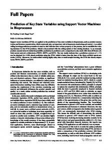
Fig. 6.

Online estimation results for a representative hyperventilation case. I/O configuration No. 3 was applied to data set No. 10. (A) The input, i.e., the measured ABP. (B) The estimated ICP and the measured ICP and (C) that of the CBFV. The estimated signals are virtually on top of their measured counterparts. Hyperventilation started around the fifth minute that caused a decrease of ICP and CBFV as expected.


Hu et al.

Page 27


Fig. 7.

Online estimation results for a representative hyperventilation case. I/O configuration No. 3 was applied to data set No. 10. (A) The unobserved r1 together with its ±3 STD limit and (B) that of r2. It should be noted that estimated standard deviation of r1 is too small such that its ±3 STD limit cannot be shown in this scale.


Hu et al.

Page 28


Fig. 8.

Offline fitting results for a representative propofol case. I/O configuration No. 3 was applied to data set No. 1. (A) The fitted ICP superimposed on the measured one at the end of the offline fitting while (B) is that of the CBFV.


Hu et al.

Page 29


Fig. 9.

Online estimation results for a representative propofol case. I/O configuration No. 3 was applied to data set No. 1. (A) The input, i.e., the measured Pa. (B) The estimated ICP and the measured ICP and (C) that of the CBFV. The estimated signals are virtually on top of their measured counterparts except after the sixteenth minute. Propofol infusion started around the fourteenth minute that caused a decreases of ICP and CBFV as expected.


Hu et al.

Page 30


Fig. 10.

Online estimation results for a representative propofol case. I/O configuration No. 3 was applied to data set No. 1. (A) The unobserved r1 together with its ±3 STD limit and (B) that of r2.



1 2 3 4 5 6 7 8

IAH: Intracerebral hemorrhage.

SDH: Subdural hematoma.

SAH: Subarachnoid hemorrhage.

GOSE12: Twelve month Glasgow Outcome Score extended.

GOSE3: Three month Glasgow Outcome Score extended [43].

M F M F M M M M

Gender

GCS: Glasgow Coma Scale at measurement [42].

58 57 68 59 25 29 47 21

Age

NIH-PA Author Manuscript Left frontal SDH Left frontal SAH Brain Stem injury Left frontal contusions SAH SAH in left sylvian fissure Bilateral frontal IAH Basal ganglia punctate hemorrhage

Diagnosis

TABLE I

8 6 4 8 6 3 7 7

GCS 3 3 Dead 3 3 8 3 3

GOS3


Key Patient Characteristics

5 5 7 3 3

6 3

GOS12

Hu et al. Page 31


NIH-PA Author Manuscript TABLE II



contamination. S.D. stands for the standard deviation from these twenty-five runs.

r1(0) r2(0) x1(0) x2(0) Ga1 τ1 Ga2 τ2 Go Ke Cm Kv2 rMCA0 Tm,2 sim1 0.65 0.25 1.63 123.74 1.60 1.86 0.37 0.09 0.09 0.58 0.13 0.00 0.06 0.02 0.32 0.37 0.72 125.64 0.81 0.69 0.11 0.11 0.17 0.55 0.08 0.00 0.12 0.01 S.D. sim2 0.44 0.33 4.00 124.07 0.91 1.70 91.44 0.38 1.52 0.29 14.76 0.00 0.28 1.54 0.45 0.33 3.82 205.00 0.02 0.17 3.54 0.03 0.97 0.07 11.60 0.00 0.01 0.08 S.D. sim3 0.37 0.04 32.45 15.09 224.50 0.10 0.63 0.16 0.42 0.32 0.12 0.02 0.08 0.36 0.34 0.02 35.55 15.31 135.36 0.07 0.37 0.09 0.18 0.15 0.07 0.02 0.01 0.05 S.D. sim4 0.63 0.28 0.62 24.97 0.97 0.92 13.18 0.29 0.27 0.18 0.73 0.00 0.21 1.04 0.34 0.31 0.40 26.31 0.01 0.35 3.43 0.11 0.15 0.12 0.80 0.00 0.02 0.06 S.D. sim5 0.67 0.53 5.69 14.02 0.41 0.26 3.72 0.20 0.29 0.24 0.08 0.07 0.06 0.12 0.31 0.44 4.78 12.85 0.28 0.27 3.33 0.17 0.15 0.38 0.13 0.00 0.05 0.03 S.D. sim1 through sim5 represent five simulation experiments based on the data from five different patients. For each experiment, twenty-five runs were performed with independent observation noise

List of Average Normalized Parameter Estimation Error Obtained by Fitting the Model With the Third I/O Configuration. Results Were Averaged From 25 Independent Runs Hu et al. Page 32


NIH-PA Author Manuscript TABLE III



Sim r2 0.39 0.21 0.22 0.12 0.10 ICP 0.36 0.00 0.17 0.20 −0.38

r1 0.48 0.73 0.76 0.62 0.72

KF r2 0.85 −0.78 0.74 0.10 0.45 ICP 0.98 0.87 0.91 0.85 0.49

r1 0.53 0.78 0.79 0.63 0.90

QPKF r2 0.90 −0.85 0.74 0.09 0.71 ICP 0.96 0.84 0.90 0.86 0.74

QPKF: calculate state variables by using the DD1 filter with the Kalman gain solved using the quadratic programming

KF: calculate state variables by using the DD1 filter

Sim: calculate state variables by a pure simulation

noise contamination.

Notations of sim1 through sim5 represent five simulation experiments based on the data from five different patients. For each experiment, twenty-five runs were performed with independent observation

sim1 sim2 sim3 sim4 sim5

r1 0.17 0.28 0.21 0.16 0.23

List of Average Cross Correlation Coefficients Between True State Values and Their Estimates by Running Three Different State Estimation Methods With Model Parameters Identified in Table II Plus Additional 3% Perturbation on the Initial Values of State Variables. Results Were Averaged From 25 Independent Runs

Hu et al. Page 33


NIH-PA Author Manuscript TABLE IV



0.93 0.47 0.62

0.85 0.19 0.43

I/O1 r2 0.78 −0.88 0.67 0.86 0.46 0.44

ICP 0.36 0.24 0.75

I/O3: The third I/O configuration

I/O2: The second I/O configuration

I/O1: The first I/O configuration

sim3 sim4 sim5

sim∗ 2

sim1 sim2

r1 0.39 0.44 0.74 0.98 0.74 0.81

r1 0.46 0.30 0.93 0.88 0.38 0.46

I/O2 r2 0.84 −0.53 0.62 0.98 0.80 0.84

CBFV 0.89 0.66 0.81 0.86 0.68 0.91

r1 0.54 0.78 0.93 0.74 0.07 0.71

I/O3 r2 0.90 −0.85 0.84 0.90 0.86 0.73

ICP 0.96 0.83 0.98

Results Similar to Those Reported in Table III Except That Three I/O Configurations Were Compared Using the Quadratic Programming Kalman Filter. Results for 2* Were Obtained Using the True Model Parameters Plus 3% error in Initial Values Hu et al. Page 34


NIH-PA Author Manuscript TABLE V

NIH-PA Author Manuscript Data set# cICP cCBFV

1 −0.59 0.35

2 −0.76 0.75

3 −0.64 0.34

4 0.06 0.79

5 −0.36 1 0.18

6 −0.44 0.22

7 0.35 0.43

8 −0.45 0.39

9 0.39 0.70

10 −0.86 −0.17

cCBFV: Spearman correlation coefficient between measured CBFV and estimated CBFV using the second I/O configuration with the quadratic programming Kalman filter.

cICP: Spearman correlation coefficient between measured and estimated ICP using the first I/O configuration with the quadratic programming Kalman filter.

I/O configuration# 1 2

11 −0.83 −0.12


List of State Estimation Results From Processing Eleven Data Sets From Real Patient Recordings Using the QPKF Filter Hu et al. Page 35


Hu et al.

Page 36

TABLE VI

list of baseline values of model parameters Parameter Values


r0,1 = 0.015 cm h0,1 = 0.003 cm σe0,1 = 0.1425 mmHg Kσ,1 = 10 σcoll,1 = 62.79 mmHg T0,1 = 2.16 mmHg cm rm,1 =0.027 cm rt,1 = 0.018 cm nm,1 = 1.83 cm η1 = 232 mmHg s Kg,1 = 1.43e6 (mmHg s cm)−1 Kv,1 = 4.64e3 cm τ1 = 10 s Ga1 = 0.02 mmHg−1 Gpv = 1.136 mmHg−1 s−1 ml Gf = 4.2e − 4 mmHg−1 s−1 ml Ke = 0.11 ml−1 Pan = 100 mmHg qn = 12.5 ml s−1 Krmca = 5

r0,2 = 0.0075 cm h0,2 = 0.00025 cm σe0,2 = 11.19 mmHg Kσ,2 = 4.5 σcoll,2 = 41.32 mmHg T0,2 = 1.50 mmHg cm rm,1 = 0.0128 cm rt,2 = 0.0174 cm nm,2 = 1.75 cm η2 = 47.8 mmHg s Kg,2 = 1.02e8 (mmHg s cm)−1 Kv,2 = 154.32e3 cm τ2 = 20 s Ga2 = 5.2 mmHg−1 rMCAo = 0.14 cm Go = 1.9e − 3 mmHg−1 s−1 ml Cm = 0.2 mmHg−1 ml Picn = 9.5 mmHg Ps = 6.0 mmHg

NIH-PA Author Manuscript NIH-PA Author Manuscript Conf Proc IEEE Eng Med Biol Soc. Author manuscript; available in PMC 2007 December 19.

Estimation of Hidden State Variables of the Intracranial System Using ...

Estimation of Hidden State Variables of the Intracranial System Using ...

Suggest Documents

State Space Model with hidden variables for reconstruction of gene ...

Distribution System State Estimation

Advantages of power system state estimation using ... - CiteSeerX

Learning with hidden variables

INSTRUMENTAL VARIABLES ESTIMATION OF HETEROSKEDASTIC ...

Instrumental variables estimation using ... - Boston College

Efficient estimation of hidden state dynamics from spike ... - CiteSeerX

Battery State of Charge Estimation Using

Battery State-of-Charge Estimation Using ...

estimation of plausible values using background variables with ...

Dryness Estimation using Three Variables of Land ...

Stratified estimation of forest inventory variables using spatially ...

Accurate automatic estimation of total intracranial ...

Unconditional no-hidden-variables theorem

Estimation of sums of random variables - arXiv

Cryptography and System State Estimation Using ... - Semantic Scholar

Low voltage system state estimation using smart meters - IEEE Xplore

Low Voltage System State Estimation Using Smart Meters - IEEE Xplore

Intracranial variables in propofol/sevoflurane-anesthestized ... - Scielo.br

State estimation for nonlinear system diagnosis using multiple models ...

State Estimation for Anaerobic Digesters using the

State and Parameter Estimation of The Lorenz System In

Using a state-space model with hidden variables to infer transcription ...

Prediction of Key State Variables using Support Vector Machines in