For applications of these es- timators ... Cline and Hart (1991), and van Es (1992). ... Here the function (x) is defined and Lipschitz continuous on 0 1], and (x) is.
Statistica Sinica
6(1996),
79-95
ESTIMATION OF JUMP POINTS AND JUMP VALUES OF A DENSITY FUNCTION C. K. Chu and P. E. Cheng National Tsing Hua University and Academia Sinica Abstract: The estimation of locations of jump points and corresponding jump sizes
of a density function on a bounded interval of interest by the kernel method is considered. Strong convergence rates (SCR) and limiting distributions for the proposed estimators are obtained. The order of the SCR for estimators of locations for jump points is immune to the smoothness conditions imposed on the density function, but that for estimators of jump sizes is not. The limiting distributions are used to test the continuity of the density function and give asymptotic con dence intervals for locations of jump points and corresponding jump sizes. For applications of these estimators, the choices of bandwidths and kernel functions are considered. In the case that the number of jump points on a bounded interval of interest is known in advance, an approach is proposed to recover the density function on the interval such that the performance of the resulting density function estimate is not a�ected by these jump points. Simulations demonstrate that the asymptotic results hold for reasonable sample sizes. Key words and phrases: Asymptotic normality, density estimation, jump point, jump size, kernel estimator, strong consistency.
1. Introduction
The problem of detecting and measuring discontinuity of an unknown density function arises in many statistical applications in science and technology, such as image processing, pattern recognition, tomography, etc. In X-ray transmission tomography, Johnstone and Silverman (1990) investigate discontinuities, in the form of sharp jumps, in the tissue density across the boundaries of various regions. It is noted in their work and the references cited therein that a di�culty with such practical examples is the assessment of the adequacy of a mathematical model for the physical process encountered. In essence, discontinuity detection together with density function estimation aims at an approximate image construction in practice. So far in the statistics literature, most theoretical studies have considered analyzing discontinuity in the 1-dimensional marginal densities as a basic starting point. In this connection, the method of nonparametric kernel density estimation
80
C. K. CHU AND P. E. CHENG
(cf. Silverman (1986) and Hardle (1990)) is a reasonably useful tool for exploiting the density structure, and is often simpler and more e�ective than using a seemingly correct parametric modeling. When discontinuities are involved, their e�ects on the asymptotic behavior of the kernel density estimator and, in particular, on an optimally chosen bandwidth have been studied by van Eeden (1985), Cline and Hart (1991), and van Es (1992). Rigorous theoretical analyses, by kernel density estimation, for locations and jump sizes of the discontinuities are yet unavailable. Lee (1990) has proposed algorithms for estimating an input signal density together with nding the discontinuity locations. In the related eld of nonparametric regression, the problem of estimating the regression curve admitting jump discontinuities has been discussed by Yin (1988), Qiu et al: (1991), Muller (1992), and Wu and Chu (1993), but it is di�erent from the problem of estimating the image intensity. The method considered here for the latter problem is similar to those applied for the former. The limited goal of this study is to demonstrate that kernel density estimation can be skillfully employed in analyzing locations and jump sizes of the discontinuities of a 1-dimensional density. It is plausible that an extension of our method disigned in Section 2 would provide us with a rough idea of where the discontinuity edges or curves in a 2-dimensional image density are, although we feel that a carefully designed semiparametric approach could generate better insights and results in practice; the latter still demands further research (cf. Silverman et al: (1990)). The organization of this paper is as follows. Section 2 describes the motivation and the precise formulation of the proposed estimators of locations of jump points and corresponding jump sizes of a density function. Section 3 gives strong convergence rates (SCR) and limiting distributions for these estimators. The order of the SCR for estimators of locations of jump points can be made close to n;1 . It is immune to the smoothness conditions imposed on the density function, but that for estimators of jump sizes is not. The limiting distributions are used to test the continuity of the density function and give asymptotic con dence intervals for locations of jump points and corresponding jump sizes of the density function on a bounded interval of interest. For applications of the proposed estimators, the choices of bandwidths and kernel functions are considered. In the case that the number of jump points on a bounded interval of interest is known in advance, an approach is proposed to recover the density function on the interval. The performance of the resulting density function estimate is not a�ected by these jump points. Section 4 contains simulation studies which support our theoretical ndings. Finally, sketches of the proofs are given in Section 5.
JUMP ESTIMATION ON DENSITY FUNCTION
81
2. The Proposed Estimators
Suppose without loss of generality that the density function f de ned on the real line R has a few points of discontinuity on the bounded interval say, [0; 1]. We are interested in estimating locations and jump sizes of the jump points in [0; 1] based on a random sample X1 ; : : : ; Xn from f . Note that f might have points of discontinuity outside of [0; 1], but we are not interested in detecting these jump points. Let the density function f (x), for x 2 [0; 1], be expressed by
f (x) = � (x) + (x):
(2:1)
Here the function �P (x) is de ned and Lipschitz continuous on [0; 1], and (x) is de ned by (x) = pj=1 dj I[tj ;1) (x), for x 2 [0; 1]. Note that p is a nonnegative integer representing the number of jump points of f on [0; 1], tj are locations of jump points, tj 2 [�; 1 ; � ], and dj are nonzero real numbers representing jump sizes of f at tj . Here � is an arbitrarily small positive constant. If p = 0, then f is continuous. For simplicity of presentation, let dp+1 = 0 and jdj j > jdj+1 j, for j = 1; 2; : : : ; p. Also, assume that the distance between any two of these tj is greater than � . To construct the estimators t^j and d^j of tj and dj , respectively, for j = 1; 2; : : : ; �, the kernel density estimator is considered. Here � is a given positive integer since the true value of p is unknown. Given the bandwidth h and the kernel function K as a Lipschitz continuous probability density function supported on the interval [;1; 1], the kernel density estimator f^(x) for f (x) is given by
f^(x) = n;1
n
X
i=1
Kh(x ; Xi );
(2:2)
for x 2 R, where Kh (�) = h;1 K (�=h). The rest of this section is devoted to formulating the proposed estimators t^j and d^j , for j = 1; 2; : : : ; �. To estimate tj , we rst consider the magnitude of f^(x), for x 2 [0; 1]. By (2.1) and (2.2), through a straightforward calculation, we have f^(x) = E [f^(x)] + f^�(x); for x 2 [0; 1], where
E [f^(x)] = � (x) +
p
X
j =1
dj
Z
(x;tj )=h
;1
K + O(h);
f^�(x) = f^(x) ; E [f^(x)]:
82
C. K. CHU AND P. E. CHENG
Lemma 2.1.2 of Prakasa Rao (1983) shows that f^� (x) converges to 0 uniformly with probability one, in both cases of p = 0 and p > 0. This implies that f^�(x) is of small order in magnitude, for all x 2 [0; 1], asymptotically. Thus, the e�ect of jump points on the magnitude of f^(x) will only appear in the value of E [f^(x)]. Also, to consider the magnitude of f^(x), it is enough to consider that of E [f^(x)]. Accordingly, to discover tj by kernel density estimation, we construct a function J (x) de ned by J (x) = f^1 (x) ; f^2(x); for x 2 [0; 1]. Here f^1 (x) and f^2 (x) are kernel density estimators for f (x) with di�erent kernel functions K1 and K2 , respectively, and the same bandwidth h. From the above results, we nd that the magnitude of jJ (x)j can be asymptotically expressed by jJ (x)j = jE [f^1 (x) ; f^2(x)]j + Op(n;1=2 h;1=2) p
X
=
j =1
dj
Z
(x;tj )=h
;1
(K1 ; K2 ) + O(h) + Op (n;1=2 h;1=2 );
(2:3)
for x 2 [0; 1]. To nd locations of jump points tj , some basic conditions imposed on K1 and K2 would beR bene cial. Let K1 and K2 satisfy K2 (z) = K1 (;z ), R R K1 = K2 = 1, and ;01(K1 ; K2 ) 6= 0. Given these K1 and K2 , through a straightforward calculation, two results for the asymptotic value of jJ (x)j easily follow. It is symmetric about tj and convex downward on some neighborhood of tj , for each j = 1; 2; : : : ; p. The widths of these neighborhoods of tj correspond to those of the intervals where K1h and K2h are supported. On the other hand, it is zero outside of the union of these neighborhoods of tj . Based on the above characteristics of the magnitude of jJ (x)j, we propose to take local maximizers of jJ (x)j as estimators of locations of jump points. Since K1 and K2 are supported on [;1; 1], the widths of the above neighborhoods of tj are not greater than 2h. Combining this result with the fact that jdj j > jdj+1 j, for j = 1; 2; : : : ; p, we take t^j as maximizers of jJ (x)j over the sets Aj , where
Aj = [0; 1] ;
j[ ;1 k=1
[t^k ; 2h; t^k + 2h];
for j = 1; 2; : : : ; �. We now give the formulation of d^j . To estimate dj , based on the above t^j , a direct method is to take the rescaled J (t^j ) as d^j , for j = 1; 2; : : : ; �. By (2.3), the R0 scale factor cJ for J (t^j ) is cJ = [ ;1 (K1 ; K2 )];1 . However, there is a drawback to this simple approach. To address this drawback, consider the case t^j = tj + �h, for some j and � 6= 0. Then, based on the above arguments, the value of d^j is
JUMP ESTIMATION ON DENSITY FUNCTION
83
asymptotically equal to cJ dj ;�1 (K1 ; K2 ) which is not equal to dj for 0 < j�j < 1 and is equal to 0 for j�j � 1. By this, the drawback to the simple approach is that, even though t^j is close to tj , dj can not be estimated well. To address the above drawback to the simple approach, we propose taking the rescaled S (t^j ) as d^j , for j = 1; 2; : : : ; �. The function S (x) is de ned by S (x) = f^3(x) ; f^4(x); R
for x 2 [0; 1]. Here f^3 (x) and f^4 (x) are kernel density estimators for f (x) with di�erent kernel functions K3 and K4 , respectively, and the same bandwidth g. Note that K3 and K4 satisfy the above conditions given on K1 and K2 , respectively, and the value of g is of larger order than that of hR . Based on the above arguments, the scale factor cS for S (t^j ) is taken as cS = [ ;01 (K3 ; K4 )];1 . We now give the e�ect of the order of magnitude of g on the performance of the proposed d^j . Consider the above case t^j = tj + �h, for some j and � 6= 0. R �h=g Following the same arguments, the value of d^j is roughly equal to cS dj ;1 (K3 ; K4 ) which approaches dj as h=g approaches 0, for each � 6= 0. Combining this result with the fact that the value of g is of larger order than that of h, the proposed d^j does not have the above drawback. Finally, the asymptotic behaviors of the proposed estimators t^j and d^j of tj and dj , respectively, will be studied in Section 3. For applications of the proposed estimators, the choices of bandwidths and kernel functions will be considered in Remark 2 of Section 3.
3. Results
In this section, we shall study the asymptotic behaviors of t^j and d^j , for j = 1; 2; : : : ; �. For these, we impose the following assumptions: (A.0) X1 ; : : : ; Xn are independence random variables with density function f (x) as given in (2.1). (A.1) The qth derivative � (q) of � in (2.1) is Lipschitz continuous on the interval [0; 1], where q � 2. Here and throughout this paper, the notation m(j) denotes the j th derivative of the given function m, for some integer j � 0. (A.2) The kernel function K1 is supported on the interval [;1; �], � 2 [0; 1], and of order q.R Recall that a kernel function G Ris said to be of order q if it satis es R G = 1, z`G = 0, for 1 � ` < q, and zq G 6= 0. Also, K1(1) is Lipschitz continuous, K1(1) (0) 6= 0, and K1(`) (;1) = K1(`) (�) = 0, for ` =R 0; 1. The kernel function K2 is de ned by K2 (z ) = K1 (;z ),R for all z . Finally, ;01 (K1 ; K2 ) 6= 0 and there is a constant � > 0 such that j 0cn (K1 ; K2 )j > �c�n , for some � � 2 and any sequence cn of positive real numbers converging to 0 as n ! 1.
84
C. K. CHU AND P. E. CHENG
(A.3) The kernel function K3 is supported on the interval [;1; !], ! 2 [0; 1], Lipschitz continuous, and of order q. The kernel function K4 isR de ned by K4 (z ) = K3 (;z ), for all z. The kernel functions K3 and K4 satisfy ;01(K3 ; K4 ) 6= 0. (A.4) The total number of observations in this density estimation setting is n, with n ! 1. The bandwidths h = hn and g = gn satisfy h ! 0 with nh ! 1, and g ! 0 with ng ! 1, as n ! 1. Theorems 1 and 2 below will give the asymptotic behaviors of t^j and d^j in the cases p � � � 1 and � > p � 0, respectively. The proofs of these theorems are given in Section 5. To state these theorems, we need the following notation. Let = 2[q=2] + 1, �j = ((n=h)1=2 (t^j ; tj ), (ng)1=2 (d^j ; dj ))T , for j = 1; 2; : : : ; �, � a positive constant, where � 2 (0; =�), and � an arbitrarily small positive constant. Here the notation [x] denotes the largest integer which is smaller than x, and T the transpose of a vector. In these theorems, some conditions on the values of n, h, g, �, and � include: (B.1) (B.2) (B.3) (B.4) (B.5) (B.6) (B.7)
n;1+� h;1;2�� = o(1); n1;� g;1 h2+2� = o(1); n1;� g1+2 = o(1); n h1+2 = o(1); n g;1 h2+2� = o(1); n g1+2 = o(1); h g;1 = o(1):
Theorem 1. In the case p � � � 1, under the above assumptions (A.0) through (A.4), if (B.1) holds, then P (jt^j ; tj j > h1+� i:o:) = 0; for j = 1; 2; : : : ; �. Also, if (B.1) through (B.3) hold, then n(1=2);� g1=2 jd^j ; dj j ! 0 a:s:;
(3:1) (3:2)
for j = 1; 2; : : : ; �. Furthermore, if (B.1) and (B.4) through (B.7) hold, then
�j ) N
�
(0; 0)T ;
�
d;j 2Fj U
0
��
0 Fj V ; for j = 1; 2; : : : ; �, and these �j are asymptotically independent, where
Fj = (1=2)[f (t;j ) + f (t+j )];
(3:3)
JUMP ESTIMATION ON DENSITY FUNCTION
85
Z
U = [ (K1(1) ; K2(1) )2 ] = [2K1(1) (0)]2 ; Z
V = [ (K3 ; K4
Z
)2 ] = [
0
;1
(K3 ; K4 )]2 :
Theorem 2. In the case � > p � 0, under the above assumptions (A.0) through (A.4), if (B.1) through (B.3) hold, then
n(1=2);� g1=2 jd^j ; dj j ! 0 a:s:
(3:4)
for j = 1; 2; : : : ; �. Here dj = 0, for j > p. The following Theorem 3 will give a con dence band for jJ (x)j. Using this con dence band, the test of the null hypothesis H0 : p = 0 against the alternative hypothesis H1 : p > 0 on the interval [a; b] can be performed. Theorem 3 is obtained directly from (1.2) of Bickel and Rosenblatt (1973). Hence its proof is omitted. Theorem 3. Under the above assumptions (A.0) through (A.4), if f (q) is Lipschitz continuous on the interval [a; b] and h = n; , where 2 (1=3; 1) for q = 0 and 2 ((2q + 1);1 ; 1) for q � 1, then
P ( sup jJ (z )j < an + bn x) ! exp(;2 exp(;x) ); z2[a;b]
where Z
h
Z
i
an = wn hab + h;ab1 log( (2�);1 ( (K1(1) ; K2(1) )2 = (K1 ; K2 )2 )1=2 ) ; bn = wn h;ab1; and
i1=2 hZ 0 i;1 2 wn = (K1 ; K2 ) (K1 ; K2 ) ; ;1 hab = [2 log((b ; a)=h)]1=2 : h
n;1h;1 f^1(x)
Z
We now close this section by the following remarks. Remark 1. By (3.1) and (B.1), if � = 2, � = �, and h = �1n;1+5� , �1 > 0, then the order of the SCR for t^j is n;1+4� . This order of the SCR for t^j is independent of the value of q. Hence the smoothness condition imposed on the continuous part � of f does not e�ect this order of the SCR for t^j . On the other hand, by (3.2) and (B.1) through (B.3), if g = �2 n(;1+�)=(1+2 ), �2 > 0, and the above values of �, �, and h are given, then the order of the SCR for d^j is n; =(1+2 )+� .
86
C. K. CHU AND P. E. CHENG
Since the value of in (B.3) depends on q, the smoothness condition imposed on � has di�erent e�ects on the order of the SCR for d^j . Remark 2. In the case p � � � 1, to estimate tj and dj , for j = 1; 2; : : : ; �, a possible approach for practical choice of bandwidths and kernel functions is now given. Van Es (1992) has shown that the magnitude of the least squares cross-validated bandwidth produced in the case p > 0 is of order n;1=2. By virtue of this, to estimate tj , we suggest taking h as the least squares cross-validated bandwidth. Theoretically, given this value of h, � = 2, and � = (1=4) ; �, then the SCR of t^j to tj is of order n(;5=8)+� . To choose K1 and K2 , by (5.8), (A.2), and (B.1), t^j have asymptotic mean square errors n;1 hd;j 2 Fj U (1 + o(1)). According to this, we suggest taking K1 and K2 to satisfy the conditions given in (A.2) and minimize the value of U over the class of (q + 4)-th degree polynomials. For example, in the case q = 0,
K1(x) = (0:4857;3:8560x+2:8262x2 +19:1631x3 +11:9952x4 )I[;1;0:2012] (x) (3:5) and K2 (x) = K1 (;x), for all x. The reason for choosing K1 in the class of (q + 4)-th degree polynomials is that, by (A.2), it must satisfy the following q + 4 R R conditions K1 = 1, z ` K1 = 0, for 1 � ` � q ; 1, and K1 (;1) = K1(1) (;1) = K1 (�) = K1(1)(�) = 0. The same remark applies to K2. To estimate dj , we suggest choosing g as the least squares cross-validated bandwidth produced from the data in some subinterval [a; b] of [0; 1] on which the hypothesis test given in Theorem 3 has been performed and the null hypothesis accepted. The magnitude of the resulting g is of order n;1=(1+2q) . For this, see, for example, Hall and Marron (1987). Theoretically, given this value of g and the above values of h, �, and � chosen for estimation of tj , the SCR of d^j to dj is of order n(;q=(1+2q))+� . This order is close to the optimal rate of uniformly strong consistency of f^ to f in the case p = 0 given in Hardle (1991). Unfortunately, we do not know how to optimally choose K3 and K4 . Finally, the performance of t^j and d^j derived by this approach needs further study. Remark 3. We now consider the estimation of the density function f (x), for x 2 [0; 1], when the value of p in (2.1) is known in advance. For this, using the results of Theorem 1 and Remark 2 in Section 3, the loctions of jump points can be estimated accurately, in the sense of SCR. In this case, we propose to estimate the density function by a kernel density estimator on subintervals separated by these estimates of locations of jump points. To avoid boundary e�ects on the kernel density estimator, the boundary modi cation method given in Gasser and Muller (1979) is applied. Through a straightforward calculation, the performance of the resulting kernel density estimate is the same as that given in Hardle (1991)
JUMP ESTIMATION ON DENSITY FUNCTION
87
for the case that the density function has q Lipschitz continuous derivatives, in the sense of the mean integrated square error over the interval [0; 1]. Remark 4. We now consider an intuitively simple estimation idea compared to the approach proposed above. If K1 and K2 are taken as the uniform kernel functions K1 (x) = I[;1;0] (x) and K2 (x) = I[0;1] (x), then t^j are simply constructed by comparing the number of data points within an interval of length h to the left of a location and that within a similar interval to the right. In this case, (3.1) still holds. Note that these rectangular kernel functions K1 and K2 exhibit jump points at endpoints of their support. In general, kernel functions with jump points will lead to bad nite sample behaviors of kernel estimators (see for example, Section 2.1 of Hardle (1991)). By this, the resulting jJ (x)j might have more local maximums (or sparks) than that using smooth kernel functions. The former will more often produce incorrect estimates of tj than the latter. Simulation results given in Section 5 demonstrate that such particular t^j are inferior to the ones using other proper choices of K1 and K2 , in the sense of having larger minimum sample mean square error over h.
4. Simulations
To investigate the practical implications of the asymptotic results of the proposed estimators of locations of jump points presented in Section 3, an empirical study was carried out. The simulation settings were as follows. The sample size was n = 100. Three density functions with the same location of jump point x = 0 were considered. The density functions were f� (x) = �� (x)I[x�0] + �0:5 (x)I[x>0] , where � = 2; 1, and 2=3. The corresponding jump sizes of f� (x) at x = 0 are d(2�);1=2 , where d = 3=2; 1, and 1=2. Here �z (x) denotes the probability density function of Normal(0; z 2 ). For each density function, 100 independent sets of observations Xi were generated. Two sets of the kernel functions K1 and K2 were used. The rst were those given in (3.5). The second were the uniform kernel functions given in Remark 4. The resulting estimates of the location of the jump point are denoted by t^1 and t^�1 , respectively. We now describe the calculation of t^. Here t^ stands for t^1 and t^�1 . For each data set, the location of the jump point was searched for on the interval [;6; 2]. This interval was chosen arbitrarily. For this, 6 values of h, h = 0:03; 0:1; 0:2; : : : ; 0:5, were chosen. For each data set and each value of h, the values of jJ (x)j were calculated on an equally spaced grid of 801 values on [;6; 2]. The maximizer t^ of jJ (x)j over [;6; 2] was calculated. After evaluation on the grid, a one-step interpolation was done, with the result taken as t^. Figure 1 shows jJ (x)j with the kernel functions K1 and K2 given in (3.5) and h = 0:03 (solid curve) and h = 0:3 (dashed curve) derived from the simulated
88
C. K. CHU AND P. E. CHENG
data from f� with � = 2 (stars at the bottom). Given a small value of h = 0:03, the maximizer of jJ (x)j over the interval [;6; 2] shows the location of jump point incorrectly. On the other hand, increasing the value of h as h = 0:3, the maximizer of jJ (x)j over [;6; 2] shows the location of the jump point x = 0 accurately in this example. Based on this simulated data, we might consider that the underlying density has a peak to the right of 0, a bump in [;2; ;1], a long-left tail, and a short-right tail. It is di�cult to distinguish visually from the simulated data alone that the underlying density function has a jump point at x = 0. 1:5
1:1
0:7
0:3
;0:1 ;6
;4
;2
0
2
x
Figure 1. Plot of jJ (x)j with h = 0:03 (solid curve) and h = 0:3 (dashed curve) derived form the simulated data set (stars at the bottom).
For each density function f� (x), Table 1 gives the sample bias, standard deviation, and mean square error of t^1 and those of t^�1 in parentheses. For each f� (x), when h increased from 0.03 to 0.4, there is a tendency that t^1 moved from the right to the left. But t^�1 does not show this tendency. For each f� (x), Table 1 also shows the minimum absolute sample bias, minimum sample standard deviation, and minimum sample mean square error of t^1 and those of t^�1 in the last row. These values show the performance of the estimators with the ideal choice of the optimal bandwidth. It is clear that t^1 has smaller minimum sample
JUMP ESTIMATION ON DENSITY FUNCTION
89
mean square error over h than t^�1 , for each f� (x). Table 1. The sample bias, standard deviation (SD), and mean square error (MSE) of t^1 and those (given in parentheses) of t^�1 . f� (x)
�=2
h value
0.03 0.1 0.2 0.3 0.4 0.5
Bias
SD
MSE
0.064) 0.070) 0.037) 0.008) 0.014) 0.052)
0.266(0.307) 0.224(0.231) 0.158(0.128) 0.159(0.127) 0.107(0.147) 0.128(0.191)
0.087(0.098) 0.058(0.058) 0.029(0.018) 0.025(0.016) 0.011(0.021) 0.016(0.039)
0.004( 0.008)
0.107(0.127)
0.011(0.016)
0.028( ;0.060) 0.055( 0.006) 0.007( ;0.043) ;0.076( ;0.112) ;0.083( ;0.003) 0.034( 0.124)
0.330(0.386) 0.293(0.334) 0.365(0.344) 0.384(0.342) 0.384(0.372) 0.416(0.397)
0.109(0.151) 0.088(0.110) 0.132(0.119) 0.152(0.128) 0.153(0.137) 0.173(0.171)
0.007( 0.003)
0.293(0.334)
0.088(0.110)
;0.004( ;0.127) ;0.026( ;0.040) ;0.077( ;0.098) ;0.123( ;0.156) ;0.165( ;0.170) ;0.064( ;0.062)
0.276(0.316) 0.343(0.330) 0.395(0.363) 0.391(0.377) 0.429(0.457) 0.498(0.505)
0.075(0.115) 0.117(0.109) 0.160(0.140) 0.167(0.165) 0.210(0.236) 0.250(0.256)
0.004( 0.040)
0.276(0.316)
0.075(0.109)
0.129( 0.090( 0.068( 0.011( ;0.004( ;0.008(
min abs �=1
0.03 0.1 0.2 0.3 0.4 0.5 min abs
� = 2=3
0.03 0.1 0.2 0.3 0.4 0.5 min abs
5. Sketches of the Proofs The following notation will be used throughout this section. Set �h = (1 = 2) n ;� h1=2 and �g = n(1=2);� g1=2 . Let E [S (t^j )] = E [S (x)]jx=t^j , and E [J (1) (t^j )] = E [J (1) (x)]jx=t^j , for j = 1; 2; : : : ; �. Let zi , i 2 Z , denote partition points of
90
C. K. CHU AND P. E. CHENG
[0; 1] satisfying zi ; zi;1 = n;(1+q) , the interval [0; 1], = fi : zi 2 g, j = fx : x 2 Aj , I[jx;tj j>h � ] = 1g, and uj the partition point satisfying juj ; tj j = minfjzi ; tj j : i 2 g, for j = 1; 2; : : : ; p. To prove Theorem 1 and 2, we require the following lemma. Lemma 1. In the case p � 0, under (2.1), (A.0), and (A.1), if K is compactly supported on [;1; 1], Lipschitz continuous, and of order q, then the kernel density estimator f^(x) of (2:2) has the following properties: 1+
p
;1
j=1
uniformly on ,
(x;tj )=h
Z
X E [f^(x)] = � (x)+ dj
K + hq (;1)q � (q)(x)
Z
z q K=(q!)+ O(hq+1 ); (5:1)
�h sup jf^(x) ; E [f^(x)]j ! 0 a:s: x2
(5:2)
Proof. The proof of (5.1) follows through straightforward calculation. Hence it is omitted. We now give the proof of (5.2). For this, let f^� (x) = f^(x) ; E [f^(x)]. Consider the inequality
�h sup jf^� (x)j � '1 + '2 ; x2
where
'1 = �h sup jf^� (zi )j; i2
'2 = �h sup
sup
i2 jx;zi j�n;(q+1)
jf^�(x) ; f^�(zi )j:
The proof of (5.2) is complete by showing that 'i ! 0 a.s: for i = 1; 2. To check the strong consistency of '1 , using the result that E [f^� (x)2k ] = O(n;k h;k ) uniformly on , for any integer k � 1, and taking � > 0, then, for any k = 1; 2; : : :, there is a constant ak such that 1
X
n=1
P (�h sup jf^�(zi )j > �) � i2
1
X
n=1
ak �;2k n(1+q);2k� :
According to this result, the strong consistency of '1 follows by using the BorelCantelli lemma and the fact that there is a su�ciently large k such that (1 + q) ; 2k� < ;1. The strong consistency of '2 is a consequence of the Lipschitz continuity of K . Hence, the proof of (5.2) is complete, i.e: the proof of Lemma 1 is complete.
Proof of Theorem 1.
We rst give the proof of (3.1). The proof for t^1 is complete by showing
P ( sup jJ (x)j � jJ (u1 )j i.o.) = 0: x2 1
(5:3)
JUMP ESTIMATION ON DENSITY FUNCTION
91
To check (5.3), by (5.1), (A.1), (A.2), jdj j > jdj+1 j, for j = 1; 2; : : : ; p, and the fact that � 2 (0; =�), through straightforward calculation, then
jE [J (u1 )]j ; xsup jE [J (x)]j = d1 2 1
where
h�
Z
0
(K1 ; K2 ) + O(h ) � 2C + O(h );
C = (1=2)jd1 j�h�� :
Using this result, then, through straightforward calculation, sup jJ (x)j ; jJ (u1 )j � 2 sup jJ (x) ; E [J (x)]j ; 2C + O(h ):
x2 1
x2
Combining this inequality with (5.2), (B.1), and the fact that � 2 (0; =�), we then have P (sup jJ (x) ; E [J (x)]j + O(h ) � C i.o.) = 0: x2
Hence, the proof for t^1 is complete. We now give the proof for t^2 . The proofs for the rest of t^j follow similarly. Since the distance between any two of tj , j = 1; 2; : : : ; p, is greater than � and h = o(1), then, for su�ciently large n, we have ju2 ; t1j > 3h. Using this result and the property of t^1 in (3.1), we have
P (u2 2 [t^1 ; 2h; t^1 + 2h] i.o.) = 0: Following essentially the same proof of (5.3), through a straightforward calculation, it follows, P ( sup jJ (x)j � jJ (u2 )j i.o.) = 0: x2 2
According to the property of t^1 in (3.1) and the fact that
jt^2 ; t1j � jt^2 ; t^1j ; jt^1 ; t1j � 2h ; jt^1 ; t1j; then
P (jt^2 ; t1 j < h i.o.) = 0:
Combining these results with the de nition of 2 , we have
P (jt^2 ; t2j > h1+� i.o.) = 0: Hence the proof of (3.1) is complete.
92
C. K. CHU AND P. E. CHENG
We now give the proof of (3.2). Here we shall only give the proof for d^1 ; d1 . The proofs for the rest of d^j ; dj follow similarly. For this, subtracting and adding the terms E [S (t^1 )] and E [S (t1 )], then d^1 ; d1 = �1 + �2 + �3 ; where �1 = cS (S (t^1 );E [S (t^1 )]), �2 = cS (E [S (t^1 )];E [S (t1 )]), �3 = cS E [S (t1 )];d1 . By this, the proof that �g jd^1 ; d1 j ! 0 a.s: is complete by showing �g �1 ! 0 a.s: and �2 +�3 = o(�g;1 ). Note that the strong consistency of �g �1 follows by the result of (5.2). To check �2 + �3 = o(�g;1 ), multiplying �2 by I[jt^ ;t j�h � ] + I[jt^ ;t j