1
Estimation of Node Density for an Energy Efficient Deployment Scheme in Wireless Sensor Network Anand Seetharam1, Abhishek Bhattacharyya1, Mrinal.K.Naskar1 and Amitava Mukherjee2 1
Advanced Digital and Embedded Systems Lab, Department of Electronics and Telecommunications Engg., Jadavpur University, Kolkata 700032, India, 2 IBM India Pvt. Ltd., Salt Lake, Kolkata 700091, India, 2 Royal Institute of Technology, Stockholm 16044, Sweden E-mail:
[email protected],
[email protected],
[email protected].,
[email protected]
Abstract—Wireless sensor network is a collection of nodes which can communicate with each other without any prior infrastructure along with the ability to collect data autonomously, effectively and robustly after being deployed in an ad-hoc fashion to monitor a given area. Since these nodes communicate wirelessly one major problem often encountered in sensor network is obtaining an optimal balance among the number of nodes deployed, energy efficiency and lifetime. In this paper we propose an effective method to estimate the number of nodes to be deployed in a given area for a predetermined lifetime so that total energy utilization and 100% connectivity are ensured. This scheme also guarantees that during each data collection cycle, each node dissipates the requisite minimum amount of energy, which also minimizes the number of nodes required to achieve a desired network lifetime. Extensive simulations have been carried out to establish the effectiveness of the scheme. Keywords—Wireless sensor network, coverage, connectivity, equal energy dissipation, idle and sleep times.
I. INTRODUCTION
W
IRELESS sensor network (WSN) can be considered as a collection of mobile or static nodes which communicate with each other wirelessly and often selforganize in a cooperative manner to collect data more costeffective and efficient ways as compared to a few macro sensors [1],[5] on being deployed in an ad-hoc fashion to monitor a given area. Recent advancements in the fields of digital signal processors, short-range radio electronics and integrated electronic devices have led to the evolution of WSNs as a special type of wireless embedded networks capable of interacting with each other without any established infrastructure. Applications of sensor networks vary widely from climatic data collection, environmental monitoring, seismic and acoustic monitoring to surveillance and national security, military and health care. These integrated nodes constituting the WSNs being highly energy constrained, replenishing the batteries for thousands of deployed nodes is also an impractical proposition. Furthermore many energy efficient strategies [3] demand an impractically large radio-
range for maintaining full connectivity between nodes which is a practical backlog. Hence it is of utmost importance to formulate schemes which obtain an optimal balance between energy-efficiency, lifetime and connectivity. In [1] although optimal spacing of nodes has been obtained by minimizing the total energy dissipation of the network, the energy dissipation of the individual nodes has been overlooked which the most important factor is determining the network lifetime. In [2] equal energy dissipation of nodes has been given importance but the author has only considered energies involved in transmitting data packets and not those involved in the receiving and idle states. Consideration for a two-dimensional network appears in [4] where lifetime maximization has gained precedence, again by minimizing the total energy of the network. Moreover in this paper most of the analyses have been done considering idealistic situations and no estimate of the number of nodes required to cover a desired area has been provided. A scheme for the network lifetime maximization has been outlined in [5]. The authors however have considered that only a single node is generating information while all the other nodes simply act as relays. Analysis considering energies used in the transmitting, receiving and idle states has been performed in [3] where variable radio ranges have been suggested as means for minimizing energy dissipation. However this strategy of varying the radio ranges for increasing the network lifetime sometimes an unfeasible proposition. In this paper, we develop a node deployment strategy to determine the number of nodes that are to be deployed in a given area to achieve a desired network lifetime. Furthermore the scheme also ensures that during each data collection cycle each node only dissipates the minimum amount of energy required by it to transmit the requisite number of packets. Apart from this, the scheme not only ensures complete connectivity but also full energy utilization which is an improvement upon previous works in these respects.
2 II.
ENERGY DISSIPATION MODEL
We consider a data collection network comprising of sensor nodes. Each data collection cycle of duration Td has been divided into four states for all the nodes – the transmitting, receiving, idle and sleep states. An energy dissipation model for radio communication similar to [1], [3] has been assumed. As a result the energy required per second for successful transmission of a data packet (Ets) is thus given by, Ets = et + eddn
(1)
where et is the energy dissipated in the transmitter electronic circuitry per packet per second and eddn is the amount of energy required per packet per second to transmit a packet over a distance d and n is the path loss exponent (usually 2.0≤n≤4.0). The distance, d, must be less than or equal to the radio range Rradio, which is maximum internodal distance for successful communication between two nodes. If T1 is the time required to successfully transmit a packet over a distance d then total energy to transmit a packet is Et=(et+ed dn) T1
sensors to be active in data collection while all the other nodes in that section are assumed to be kept in the sleep state. Initially we assume that during a data collection cycle each active node generates a data packet of B bits. All active nodes in a segment send data packets to the sink by relaying these packets to a node in the adjacent segment nearer to the sink. In order to maintain connectivity under all circumstances between any two nodes selected randomly in the adjacent segments, the relation Rradio = a 2 + 4b2 must be satisfied because in the worst case scenario the maximum distance between two nodes chosen randomly in the adjacent segments is going to be a 2 + 4b2 . This condition occurs when nodes at positions similar to C and D are simultaneously selected during data collection as illustrated in Fig. 1. Every node performs four major actions in data collection as described in Section II. III.
DETERMINATION OF NODE DENSITY FOR ACHIEVING A DESIRED NETWORK LIFETIME
(2)
If er is the energy required per packet per second for successful reception and if T2 is the total time required by a senor node to receive a packet then the total energy to receive a packet is Er=er T2
(3)
Similarly if eid is the energy spent per second by the nodes in the idle state and T3 is the time spent in the idle state, then, Eid=eid T3
(4)
The remaining part of the data collection cycle is spent in sleep state of duration T4, where we initially assume that no energy is dissipated. In our scheme we have also defined a performance-measuring parameter, namely the energy utilization ratio (η). The η may be defined as the ratio of the total energy used by the network during its lifetime to the total energy supplied to the network at the time of deployment. A network is said to be non-functional when a single node collapses so that relay is no longer possible. Thus η = (Eused/ET)*100% where Eused is the total energy utilized by the network during its lifetime and ET is the total energy of the nodes at the time of deployment. We consider that the given area to be monitored is a rectangle of area, A, as shown in Fig. 1. Let ‘a’ be its breadth and we divide its length into K equal divisions of width b. So we have, A = abK. The number of divisions is dependent on the number of data packets that we want to collect from the given area in one data collection cycle. We deploy different number of nodes in the various segments according to the relation obtained in (8). The nodes are assumed to distribute randomly in these segments. In each segment we take s number of
Fig.1. Example area Let Eo be the initial energy of each node deployed in the region. If Ei is the energy consumed by an active node in the ith segment in a data collection cycle, then we have, Ei = Et(K-i+1) + Er(K-i) + Eid = (et+eddn )(K-i+1)T1 + er(K-i)T2 + eidTidlei
(5)
where Tidlei is the minimum amount of time for which an active node in the ith segment must remain in the idle state during the data collection for successfully receiving and transmitting the requisite number of data packets. Therefore the duration of sleep state for an active node in the ith segment in a data collection cycle is, Tsleepi = Td - (K-i+1)T1 - (K-i)T2 - Tidlei
(6)
During the next data collection cycle another set of s nodes in each segment is selected This process is repeated until all the nodes in a segment have been selected once. The first set of s nodes is then chosen and the process is repeated all over again. We now compute the node density to be deployed in the various segments in such a manner that each active node dissipates minimum amount of energy. As the number of
3 packets transmitted by a node in ith segment during a cycle is considered to be fixed the amount of energy required for this transmission and reception of the packets is taken also as fixed. Further we take each active node to remain in the idle state only for the requisite amount of time spent by it to route the packets to a node in its neighboring segment thereby ensuring that each node spends minimum amount of energy during Td. As the energy dissipated by the active nodes in the various segments is different, in order to ensure η = 100% and to achieve the desired network lifetime with lesser number of nodes we propose the following scheme. Let ndi be the number of nodes deployed per unit area in the ith segment. Therefore the total number of nodes in the segment is ndiab. If the desired network lifetime is Tlife then we have, ndiabTdEo for 1≤ i ≤ K (7) sEi Now choosing one of the segments as reference, one can compute the node density of the remaining segments on the basis of its node density. The energy dissipated by an active node in the Kth segment is minimum as it has to transmit with the least number of packets. Hence we take it as the reference segment because the node density here being the least one can choose the desired network lifetime satisfying the condition ndKab≥s. Therefore we have, Ei ndi = ndK for 1≤ i ≤ K (8) EK Tlife =
nodes to be deployed in the area is performed in MATLAB. The values of the different parameters used in the simulation are et=1024µJ/packet/s, er=819.2µJ/packet/s, ed=2048 µJ/packet/m2/s, eid = 409.6µJ/s and Eo = 5.4kJ. Considering the model given in [3], and modifying it accordingly to be used in meaningful way in our scheme, we take the values of et, er, eid as mentioned above. The simulation is performed with data rate of 20 kbps as the commercially available motes have comparable data rates and we take T1=T2. Further we consider the area under consideration is rectangular with a = 60m. The length of the rectangle is taken as 200 m which is divided into 20 equal segments. Therefore K =20, b = 10m and d =20m while the total area under surveillance is 1.2*104m2. Apart from this we assume Tidlei to be directly proportional to the number of packets an active node in the ith segment transmits i.e., Tidlei =2K-2i+1. Fig. 2 shows the energy consumption of an active node in the various segments. Fig. 2 also gives us a fair idea why we require variable number of nodes in the various segments which is validated in Table I.
Moreover Td must satisfy the following conditions. If each node can transmit with a maximum of P packets per second then Td>K/P. Apart from this Td must also satisfy the following condition, Td ≥ KT1 + (K-1)T2 + Tidle1 (9) This is because as a node in the first segment handles the maximum number of packets the time required for it to transmit with these packets is also going to be maximum. Finally the total number of nodes (N) that are required to be deployed in the given area A can be calculated by the relation stated in equation (10).
K(K + 1) K(K −1) + eid∑Tidlei Et + Er 2 2 N = ndKab Et + eidTidleK
(10)
Thus if the values of Tidlei for the nodes in different segments are known then the value of the total number of nodes required to be deployed in the area A can be calculated. Tidlei will depend on the number of packets an active in the ith segment has to transmit and the routing technique will have an effect on it. IV.
SIMULATION RESULTS
The simulation evaluating the energy consumption of the active nodes in the various sections and the total number of
Fig.2. Energy consumption of active nodes TABLE I: Segment vs. number of nodes Segment Number
Number of Nodes
1 2 3 4 5 6 7 8 9 10 11 12 13 14 15 16 17 18 19 20
152 144 136 128 124 116 108 100 92 84 76 68 60 52 44 36 28 20 12 4
4
The number of active nodes in a segment is taken as 4 for the purpose of simulation assuming that this would provide satisfactory coverage. For this calculation shows that the number of nodes required to be deployed in the Kth segment is 3.8944. So we deploy 4 nodes in the Kth segment which gives ndk as 0.0067nodes/m2. The number of nodes in the different segments is computed and the result is rounded of in such a way that the total number of nodes in each of the segments is exactly divisible by 4 as is illustrated in Table I. The total number of nodes to be deployed in the given area to achieve the desired lifetime is calculated to be 1584 which closely matches the theoretically obtained result of 1558 from (10). To ensure the condition of (9) is satisfied we take Td = 41 seconds. Simulation with other feasible values of s has been performed with encouraging results. The area under coverage and lifetime of the network has also been varied and the results are found to tally with theoretical results. The total number of nodes in each segment is found to increase linearly as expected because Tidlei is taken to be a linear function of i. V.
DETERMINATION OF THE NODE DENSITY CONSIDERING FINITE ENERGY IN SLEEP STATE
In the practical scenario it is observed that a sensor node always dissipates a small but finite amount of energy in the sleep state. Analysis considering this situation is discussed in this section. Let es be the amount of energy dissipated in the sleep state per second by a node. Now the minimum amount of energy an active node in a the ith segment will dissipate is Ei = (et+eddn )(K-i+1)T1 + er(K-i)T2 + eidTidlei + esTsleepi
(11)
where Tsleepi =Td - (K-i+1)T1 - (K-i)T2 - Tidlei Once again to ensure that η = 100% we have deploy different number of nodes in various segments. To have a desired network lifetime Tlife we have as before, ndiabTdEo (12) ndiab s( Ei + es( − 1)Td ) s Choosing a segment as a reference (ndref) we can as before find out the node deployment densities of the different segments. Tlife =
Taking xi = Ei - esTd and y = (esab/s)Td we have, ndi ndref = xi + yndi xref + yndref xi ndi = ndref or, xref Here too we can take i=K as the reference segment and choose nd1 in such a way that the condition ndKab ≥ s is satisfied.
(13)
VI. CONCLUSION The deployment scheme considered in this paper not only has ensured that nodes dissipate minimum amount of energy during a data collection cycle, but also has taken into account that 100% energy utilization occurs thereby increasing network lifetime. Moreover the radio range is chosen in a manner that the full connectivity among nodes in adjacent segments is always maintained independent of their distribution in a segment. Apart from this, the node deployment strategy discussed has practically been deployed in places where data collection networks are required. The future works include analyzing the network performance considering packet losses and fading multipath channels and modifying the existing model to provide desired results under these circumstances. REFERENCES [1] Zach Shelby, Carlos Pomalaza-Raez, Heikki Karvonen and Jussi Haapola, “Energy Optimization in Multihop Wireless Embedded and Sensor Networks”, International Journal of Wireless Information Networks, Springer Netherlands, January 2005, vol .12, no. 1, pp. 11-21. [2] Martin Haenggi, “Energy-balancing strategies for Wireless Sensor Networks”, in the proceedings of the International Symposium on Circuits and Systems (ISCAS 2003), Bangkok , Thailand, 25-28 May, 2003, vol. 4, pp. 45-63. [3] Q.Gao, K.J.Blow, D.J.Holding, I.W.Marshall and X.H.Peng, “Radio Range Adjustment for Energy Efficient Wireless Sensor Networks”, Ad-hoc Networks Journal, Elsevier Science, January 2006, vol. 4, issue 1, pp.75-82. [4] Qi Xue and Aura Ganz, “On the Lifetime of Large Scale Sensor Networks”, Computer Communications, Elsevier Science, February 2006, vol. 29, issue 4, pp. 502-510. [5] Manish Bharadwaj, Timothy Garnett and Anantha P. Chandrakasan, “Upper Bounds on the Lifetime of Sensor Networks”, in the Proceedings of the International Conference on Communications (ICC ’01), Helsinki, Finland, June 2001, vol. 3, pp. 785-790. [6] I. F. Akyildiz, W. Su, Y. Sankarasubhramanium and E.Cayirci, “Wireless Sensor Networks : A Survey”, Computer Networks Journal, Elsevier Science, March 2002, vol. 38, pp. 393-422. [7] I. F.Akylidiz, Dario Pompili, Tommaso Melodia, “Underwater acoustic sensor networks: Research challenges”, Ad-hoc Networks Journal, Elsevier Science, January 2005, vol. 3, pp. 257-279. [8] Jie Wu,Shuhui Yang, “Coverage Issues in Sensor Networks with Adjustable Ranges”, in the proceedings of International Workshop on Mobile and Wireless Networking (MWN 2004), Montreal, Quebec, Canada, 15-18 Aug. 2004 (in conjunction with ICPP). . [9] Bang Wang, Wei Wang, Vikram Srinivasan and Kee Chiang Chua, “Information Coverage For Wireless Sensor Networks”, IEEE Communications Letters, vol. 9, no. 11, November 2005.