Estimation of Nonlinear Dynamic Panel Data Models with Individual

Hindawi Publishing Corporation Mathematical Problems in Engineering Volume 2014, Article ID 672610, 7 pages http://dx.doi.org/10.1155/2014/672610

Research Article Estimation of Nonlinear Dynamic Panel Data Models with Individual Effects Yi Hu,1 Dongmei Guo,2 Ying Deng,3 and Shouyang Wang4 1

School of Management, University of Chinese Academy of Sciences, Beijing 100190, China School of Economics, Central University of Finance and Economics, Beijing 100081, China 3 School of International Trade and Economics, University of International Business and Economics, Beijing 100029, China 4 Academy of Mathematics and Systems Science, Chinese Academy of Sciences, Beijing 100190, China 2

Correspondence should be addressed to Dongmei Guo; [email protected] Received 6 December 2013; Accepted 22 January 2014; Published 25 February 2014 Academic Editor: Chuangxia Huang Copyright © 2014 Yi Hu et al. This is an open access article distributed under the Creative Commons Attribution License, which permits unrestricted use, distribution, and reproduction in any medium, provided the original work is properly cited. This paper suggests a generalized method of moments (GMM) based estimation for dynamic panel data models with individual specific fixed effects and threshold effects simultaneously. We extend Hansen’s (Hansen, 1999) original setup to models including endogenous regressors, specifically, lagged dependent variables. To address the problem of endogeneity of these nonlinear dynamic panel data models, we prove that the orthogonality conditions proposed by Arellano and Bond (1991) are valid. The threshold and slope parameters are estimated by GMM, and asymptotic distribution of the slope parameters is derived. Finite sample performance of the estimation is investigated through Monte Carlo simulations. It shows that the threshold and slope parameter can be estimated accurately and also the finite sample distribution of slope parameters is well approximated by the asymptotic distribution.

1. Introduction Since many economic relationships are dynamic and nonlinear, nonlinear/dynamic panel data models could obtain more information from data sources than traditional models [1, 2]. For example, many researchers suggest that economic growth is a nonlinear process [3–5] and a number of empirical analyses of economic growth entail dynamic econometric models [6–9], with lagged dependent variable among the regressors. However, few researchers consider the dynamic and nonlinear relationships simultaneously and the purpose of this paper is to combine these two factors in one model. Many results exist in the theoretical literature concerning the estimation and inference for dynamic panel data models. Since the lagged dependent variables and the disturbance term are correlated due to the unobserved effects, standard least square methods could not obtain consistent estimators when the model is dynamic. To overcome this problem, Anderson and Hsiao [6] suggested that we difference the model first to get rid of the unobserved effects and then use instrumental variable (IV) estimation for the transformed

model. Nevertheless, this IV estimation method leads to consistent but not necessarily efficient estimates of the parameters because it does not use all the available moment conditions. Arellano and Bond [10] proposed a generalized method of moments (GMM) procedure that is more efficient than the Anderson and Hsiao [6] estimator. This literature is generalized and extended by Arellano and Bover [11] and Blundell and Bond [12], which are called forward orthogonal deviation and system GMM, respectively. For the latest development of dynamic panel data models, see Baltagi [13] and Han and Phillips [14] for more details. Several models could be chosen to describe the nonlinear relationship such as mixture models, switching models, smooth transition threshold models, and threshold models. In this paper threshold model is used because of wide applications in empirical researches. This model splits the sample into classes based on an observed variable—whether or not it exceeds some thresholds. In most situations, the complexity of the problem increases because the exact threshold is unknown and needed to be estimated. The estimation and inference are fairly well developed for linear models with

2

Mathematical Problems in Engineering

exogenous regressors [15–17], in which only the nondynamic case is considered. The dynamic panel threshold models have been used in empirical literature. Cheng et al. [18] examined the evidence on the conditional convergence growth theory, which extended dynamic panel data growth model to control both threshold effects and cross-section dependence. Chong et al. [19] studied the relationship between the depletion rate of foreign reserves and currency crises using threshold autoregressive model. Ho [20] applied a dynamic panel threshold model to examine whether the low-income countries catch up with the rich ones. Kremer et al. [21] considered a dynamic panel threshold model to study inflation thresholds for longterm economic growth. As Hansen’s model required that all regressors are exogenous, the method of Hansen [17] used in these papers to estimate the dynamic models may not be suitable due to the lagged dependent variables. So far, the theory of dynamic panel threshold model has not been available as we know except for Dang et al. [22]. However, the validity of the instrumental matrices is not proved. This paper proposes an estimation method for dynamic panel threshold model and our analysis mainly relies on Hansen [17], Arellano and Bond [10], and Caner and Hansen [16]. First, we prove that the orthogonality conditions considered in ordinary dynamic panel data models are also valid in nonlinear dynamic models. Second, we develop a GMM estimator of the threshold and slope parameters based on the above moment conditions. The remainder of the paper proceeds as follows. Section 2 introduces the model and notations. Section 3 discusses the estimation for the threshold and slope coefficients. Section 4 reports a Monte Carlo simulation, and Section 5 concludes.

2. Model Consider a simple AR(1) model without exogenous variables but with individual and threshold effects as shown in the following structural equation:

For simplicity, we assume that 𝑦𝑖0 is observed and let 𝑥𝑖𝑡 ≡ 𝑦𝑖,𝑡−1 . Alternatively, (1) can also be written compactly as 󸀠

𝑦𝑖𝑡 = 𝜇𝑖 + 𝑥𝑖𝑡 (𝛾) 𝛼 + 𝜀𝑖𝑡 ,

(3)

where 𝑥𝑖𝑡 (𝛾) = (𝑥𝑖𝑡 𝐼(𝑞𝑖𝑡 ≤ 𝛾), 𝑥𝑖𝑡 𝐼(𝑞𝑖𝑡 > 𝛾))󸀠 , 𝛼 = (𝛼1 , 𝛼2 )󸀠 .

3. Estimation In this section, we first consider a simple model without exogenous covariates and derive GMM based estimator for the threshold parameter 𝛾 and slope parameters 𝛼. Then we extend the simple model to cases with strictly exogenous covariates. 3.1. Estimation of Threshold and Slope Parameters. In traditional dynamic panel data model, two methods are commonly used to remove individual effect 𝜇𝑖 . One is firstdifference approach suggested by Arellano and Bond [10]; the other one is forward orthogonal deviation proposed by Arellano and Bover [11]. We will utilize the first-difference approach in the following derivation, due to the fact that it is more convenient for computation. First, we take first-difference for model (3) to get rid of the time invariant individual effects 󸀠

Δ𝑦𝑖𝑡 = Δ𝑥𝑖𝑡 (𝛾) 𝛼 + Δ𝜀𝑖𝑡 ,

(4)

where Δ denotes difference operator. If 𝛼1 = 𝛼2 , that is, there is no threshold effect, then additional instruments can be obtained in dynamic panel data models if one utilizes the orthogonality conditions that exist between lagged values of 𝑦𝑖𝑡 and the disturbance 𝜀𝑖𝑡 according to Arellano and Bond [10]. Here we prove that these orthogonality conditions are also valid in model (4) when 𝛼1 ≠ 𝛼2 . For any given t, we have either 𝑥𝑖𝑡 (𝛾) = (𝑥𝑖𝑡 , 0)󸀠 or 𝑥𝑖𝑡 (𝛾) = (0, 𝑥𝑖𝑡 )󸀠 . Consider the former one without loss of generality. Similarly, there must be two cases in the period 𝑡 − 1, 󸀠

𝑦𝑖𝑡 = 𝜇𝑖 + 𝛼1 𝑦𝑖𝑡−1 𝐼 (𝑞𝑖𝑡 ≤ 𝛾) + 𝛼2 𝑦𝑖𝑡−1 𝐼 (𝑞𝑖𝑡 > 𝛾) + 𝜀𝑖𝑡 , for 𝑖 = 1, . . . , 𝑁;

𝑡 = 1, . . . , 𝑇,

Case 1: 𝑥𝑖,𝑡−1 (𝛾) = (𝑥𝑖,𝑡−1 , 0) .

𝑞𝑖𝑡 ≤ 𝛾,

𝑦𝑖𝑡 = 𝜇𝑖 + 𝛼2 𝑦𝑖𝑡−1 + 𝜀𝑖𝑡 ,

𝑞𝑖𝑡 > 𝛾.

(5)

Then first difference yields

where 𝑖 denotes cross-sections and 𝑡 denotes time. 𝑦𝑖𝑡 denotes the observable dependent variable; 𝑞𝑖𝑡 denotes the exogenous threshold variable; 𝛾 denotes the threshold parameter, which is assumed to be unknown and needs to be estimated; 𝛼𝑗 denotes a parameter that satisfies |𝛼𝑗 | < 1 (𝑗 = 1, 2); 𝜇𝑖 is the unobserved individual effect; 𝜀𝑖𝑡 is the idiosyncratic error, which is assumed to be independent and identically distributed (i.i.d) with mean zero and variance 𝜎2 conditional on 𝜇𝑖 , 𝑦𝑖,𝑡−1 , . . . , 𝑦𝑖0 . 𝐼(⋅) is indicator function. One can also write (1) in the form 𝑦𝑖𝑡 = 𝜇𝑖 + 𝛼1 𝑦𝑖𝑡−1 + 𝜀𝑖𝑡 ,

󸀠

Case 2: 𝑥𝑖,𝑡−1 (𝛾) = (0, 𝑥𝑖,𝑡−1 ) .

(1)

(2)

󸀠

Δ𝑥𝑖𝑡 (𝛾) = {

(Δ𝑥𝑖,𝑡 , 0) , for case 1, 󸀠 (𝑥𝑖,𝑡 , −𝑥𝑖,𝑡−1 ) , for case 2.

(6)

Correspondingly, 󸀠

Δ𝑥𝑖𝑡 (𝛾) 𝛼 = {

𝛼1 Δ𝑥𝑖,𝑡 = 𝛼1 𝑥𝑖,𝑡 − 𝛼1 𝑥𝑖,𝑡−1 , 𝛼1 𝑥𝑖,𝑡 , −𝛼2 𝑥𝑖,𝑡−1

for case 1, (7) for case 2.

For any given 𝑡, 𝑥𝑖,𝑡−1 is a valid instrument (A valid instrument means that it should have two basic conditions: first, erogeneity, i.e., it should be independent of (or, at least, uncorrelated with) the disturbance term in the equation of interest; second, relevance, i.e., it should be correlated with the included endogenous explanatory variables for which it

Mathematical Problems in Engineering

3

is supposed to serve as an instrument.) for both case 1 and case 2 since it is correlated with Δ𝑥𝑖𝑡 (𝛾)󸀠 𝛼, that is, 𝛼1 𝑥𝑖,𝑡 − 𝛼1 𝑥𝑖,𝑡−1 or 𝛼1 𝑥𝑖,𝑡 , −𝛼2 𝑥𝑖,𝑡−1 , but not correlated with Δ𝜀𝑖𝑡 , that is, 𝜀𝑖𝑡 − 𝜀𝑖,𝑡−1 as long as 𝜀𝑖𝑡 ’s are serially uncorrelated. Given the autoregressive nature of the model and the assumption that there is no serial correlation in 𝜀𝑖𝑡 , it can be easily shown that 𝑥𝑖,1 , . . . , 𝑥𝑖,𝑡−2 are also valid instruments. Therefore, the orthogonality conditions are given by 𝐸 (𝑥𝑖,𝑡−𝑠 Δ𝜀𝑖𝑡 ) = 0,

for 𝑠 = 1, . . . , 𝑡 − 1; 𝑡 = 2, . . . , 𝑇. (8)

Define 0 𝑥𝑖1 0 𝑥𝑖,1 , 𝑥𝑖,2 0 𝑍𝑖 = ( 0 .. .. . . 0 0

⋅⋅⋅ ⋅⋅⋅ ⋅⋅⋅

0 0 0 .. .

);

𝐸 (𝑍𝑖󸀠 Δ𝜀𝑖 ) = 0.

(9)

(10)

Note that Δ𝜀𝑖𝑡 = 𝜀𝑖𝑡 − 𝜀𝑖,𝑡−1 is MA(1). Define Δ𝜀𝑖 (Δ𝜀𝑖2 , ⋅ ⋅ ⋅ , Δ𝜀𝑖𝑇)󸀠 ; then

=

𝐸 (Δ𝜀𝑖 Δ𝜀𝑖󸀠 ) = 𝜎2 𝐺,

(11)

(12)

2 −1 −1 2

𝛼̂GMM (𝛾) −1

𝑁 𝑁 { 𝑁 } 󸀠 = {[∑Δ𝑋𝑖 (𝛾) 𝑍𝑖 ] [∑𝑍𝑖󸀠 𝐺𝑍𝑖 ] [∑𝑍𝑖󸀠 Δ𝑋𝑖 (𝛾)]} 𝑖=1 𝑖=1 { 𝑖=1 }

−1

𝑁

{ } 󸀠 . {[∑Δ𝑋𝑖 (𝛾) 𝑍𝑖 ] [∑𝑍𝑖󸀠 𝐺𝑍𝑖 ] [∑𝑍𝑖󸀠 Δ𝑌𝑖 ]} , 𝑖=1 𝑖=1 { 𝑖=1 }

(13)

= [Δ𝑥𝑖2 (𝛾), . . . , Δ𝑥𝑖𝑇 (𝛾)]󸀠 , Δ𝑌𝑖 = where Δ𝑋𝑖 (𝛾) 󸀠 (Δ𝑦𝑖2 , . . . , Δ𝑦𝑖𝑇) . Stacking over individuals, (13) can be written compactly as −1

−1

󸀠

𝛼̂GMM (𝛾) = [Δ𝑋(𝛾) 𝑍(𝑍󸀠 Ω𝑍) 𝑍󸀠 Δ𝑋 (𝛾)] 󸀠

−1

where 𝑆(𝛾) = 𝑒̂(𝛾)󸀠 𝑒̂(𝛾) is the sum of squared errors. Once 𝛾̂ is obtained, we substitute the true parameter 𝛾 with its estimate 𝛾̂ yielding the feasible GMM estimator of slope coefficient estimate: 𝛾) . 𝛼̂ = 𝛼̂GMM (̂

(17)

According to Hansen [24], under the case of known 𝛾, GMM estimator 𝛼̂GMM (𝛾) is efficient and asymptotically normal: √𝑁 (̂ 𝛼GMM (𝛾) − 𝛼) 󳨐⇒ 𝑁 (0, 𝑉)

󸀠

0 0 .. ) . .

−1

(16)

as 𝑁 󳨀→ ∞,

× [Δ𝑋(𝛾) 𝑍(𝑍󸀠 Ω𝑍) 𝑍󸀠 Δ𝑌] ,

−1

−1

𝑉 = 𝑁[Δ𝑋(𝛾) 𝑍(𝜎2 𝐺) 𝑍󸀠 Δ𝑋 (𝛾)] .

Let 𝛼̂GMM (𝛾) be the GMM estimator with moment conditions given by (10). The GMM estimator can be written as

𝑁

We apply the estimator suggested by Chan [23] and Hansen [15, 17]; then 𝛾 can be estimated by

(18)

where

where

𝑁

(15)

𝛾

then for each 𝑖 the 𝑇(𝑇 − 1)/2 moment conditions described above can be written as

0 0 .. .

𝑒̂ (𝛾) = Δ𝑌 − Δ𝑋 (𝛾) 𝛼̂GMM (𝛾) .

𝛾̂ = argmin 𝑆 (𝛾) ,

d ⋅ ⋅ ⋅ 𝑥𝑖,1 , 𝑥𝑖,2 , . . . 𝑥𝑖,𝑇−1

2 −1 0 ⋅ ⋅ ⋅ −1 2 −1 ⋅ ⋅ ⋅ 𝐺 = ( ... ... ... d 0 0 0 ⋅⋅⋅ 0 0 0 ⋅⋅⋅

where Ω = 𝐼𝑁 ⊗ 𝐺, ⊗ is Kronecker product and Δ𝑋(𝛾) = 󸀠 󸀠 󸀠 ] , and 𝑍 = [Δ𝑋1 (𝛾)󸀠 , . . . , Δ𝑋𝑁(𝛾)󸀠 ] , Δ𝑌 = [Δ𝑌1󸀠 , . . . , Δ𝑌𝑁 󸀠 󸀠 󸀠 (𝑍1 , . . . , 𝑍𝑁) . In fact, this estimator is infeasible in empirical studies, since it depends on an unknown parameter 𝛾. Therefore, our next step is to estimate 𝛾 from the regression residuals:

(14)

(19)

Hansen [17] and Caner and Hansen [16] show that the dependence on the threshold estimate is not of first-order asymptotic importance, so inference on 𝛼̂ could proceed as if the estimated threshold parameter 𝛾̂ was the true parameter 𝛾. Then, √𝑁 (̂ 𝛼 − 𝛼) 󳨐⇒ 𝑁 (0, 𝑉)

as 𝑁 󳨀→ ∞.

(20)

The estimated covariance matrix becomes (One can also consider Windmeijer’s bias-corrected estimator (Windmeijer [25]) for the robust VCE of two-step GMM estimators.) −1

󸀠 ̂−1 󸀠 ̂ = 𝑁[Δ𝑋(̂ 𝑍 Δ𝑋 (̂ 𝛾)] , 𝑉 𝛾) 𝑍𝐺

(21)

̂ = ∑𝑁 𝑍󸀠 (̂ where 𝐺 𝛾)̂ 𝑒1 (̂ 𝛾)󸀠 )𝑍𝑖 and 𝑒̂1 (̂ 𝛾) = Δ𝑌 − Δ𝑋(̂ 𝛾)̂ 𝛼. 𝑖=1 𝑖 𝑒1 (̂ ̂ Similarly, one can prove that 𝑉converges in probability to 𝑉as in Caner and Hansen [16]. 3.2. Estimation of the Model with Exogenous Variables. Now we extend the results in the previous subsection to cases with strictly exogenous variables. Consider additional regressors 𝑚𝑖𝑡 in model (1): 𝑦𝑖𝑡 = 𝜇𝑖 + (𝛼1 𝑦𝑖𝑡−1 + 𝑚𝑖𝑡󸀠 𝛽1 ) 𝐼 (𝑞𝑖𝑡 ≤ 𝛾) + (𝛼2 𝑦𝑖𝑡−1 + 𝑚𝑖𝑡󸀠 𝛽2 ) 𝐼 (𝑞𝑖𝑡 > 𝛾) + 𝜀𝑖𝑡

(22)

4

Mathematical Problems in Engineering Table 1: Quantiles of distribution, 𝜃 = 0.1.

Quantiles 𝛾=2 𝑁 = 100 𝑁 = 200 𝑁 = 300 𝛼1 = 0.5 𝑁 = 100 𝑁 = 200 𝑁 = 300 𝛼2 = 0.6 𝑁 = 100 𝑁 = 200 𝑁 = 300

0.05

𝑇 = 10 0.5

0.95

0.05

𝑇 = 15 0.5

0.95

0.05

𝑇 = 20 0.5

0.95

0.10 0.89 −0.22

2.09 2.00 1.88

4.12 3.40 3.26

0.91 1.16 1.54

2.05 2.00 2.00

3.17 2.84 2.58

1.39 1.60 1.72

2.00 2.00 2.00

2.34 2.33 2.36

0.25 0.33 0.19

0.44 0.45 0.46

0.61 0.57 0.56

0.37 0.40 0.43

0.46 0.48 0.49

0.55 0.54 0.54

0.38 0.43 0.45

0.46 0.48 0.49

0.52 0.53 0.53

0.37 0.46 0.45

0.55 0.57 0.56

0.84 0.70 0.66

0.47 0.50 0.53

0.56 0.57 0.59

0.65 0.64 0.64

0.50 0.53 0.54

0.57 0.58 0.58

0.63 0.63 0.63

0.95

Table 2: Quantiles of distribution, 𝜃 = 0.3. Quantiles 𝛾=2 𝑁 = 100 𝑁 = 200 𝑁 = 300 𝛼1 = 0.5 𝑁 = 100 𝑁 = 200 𝑁 = 300 𝛼2 = 0.8 𝑁 = 100 𝑁 = 200 𝑁 = 300

0.05

𝑇 = 10 0.5

0.05

𝑇 = 15 0.5

0.95

0.05

𝑇 = 20 0.5

0.95

1.84 1.93 1.93

2.02 2.00 2.01

2.17 2.06 2.04

1.90 1.94 1.96

2.00 2.00 2.00

2.02 2.03 2.04

1.98 1.98 2.00

1.99 2.00 2.00

2.00 2.02 2.02

0.26 0.32 0.37

0.42 0.45 0.47

0.57 0.58 0.58

0.37 0.40 0.42

0.46 0.47 0.48

0.54 0.54 0.54

0.40 0.43 0.44

0.47 0.48 0.49

0.53 0.53 0.53

0.54 0.62 0.64

0.71 0.74 0.76

0.86 0.85 0.87

0.65 0.70 0.70

0.74 0.77 0.77

0.83 0.83 0.84

0.70 0.73 0.73

0.76 0.78 0.79

0.82 0.83 0.84

for 𝑖 = 1, . . . , 𝑁; 𝑡 = 1, . . . , 𝑇. Since 𝑚𝑖𝑡 are strictly exogenous, they are valid instruments for the first differenced 󸀠 󸀠 , . . . , 𝑚𝑖𝑇 ) should be added to form of (22). Therefore, (𝑚𝑖2 each diagonal element of 𝑍𝑖 in (9). Hence, the matrix of instruments is

4. Monte Carlo Experiments In this section Monte Carlo experiments are implemented to examine the finite sample performance of our estimator. For this purpose we consider the following design. 4.1. Simulation Design. The data generating process (DGP) is given by

𝑍𝑖 󸀠 𝑥𝑖1 , 𝑚𝑖2 0 󸀠 0 𝑥𝑖,1 , 𝑥𝑖,2 , 𝑚𝑖3 0 =( 0 .. .. . .

0

0

𝑦𝑖𝑡 = 𝜇𝑖 + 𝛼1 𝑦𝑖𝑡−1 𝐼 (𝑞𝑖𝑡 ≤ 𝛾) + 𝛼2 𝑦𝑖𝑡−1 𝐼 (𝑞𝑖𝑡 > 𝛾) + 𝜀𝑖𝑡 ⋅⋅⋅ ⋅⋅⋅ ⋅⋅⋅

0 0 0 .. .

)

d 󸀠 ⋅ ⋅ ⋅ 𝑥𝑖,1 , 𝑥𝑖,2 , . . . 𝑥𝑖,𝑇−1 , 𝑚𝑖𝑇 (23)

󸀠

then the estimators of 𝛾 and slope coefficients (𝛼󸀠 , 𝛽󸀠 ) can be obtained accordingly as in (16) and (17).

(24)

for 𝑖 = 1, . . . , 𝑁 and 𝑡 = 1, . . . , 𝑇, where 𝜇𝑖 ∼ i.i.d.𝑁(0, 1), 𝑞𝑖𝑡 ∼ i.i.d.𝑁(2, 1), 𝜀𝑖𝑡 ∼ i.i.d.𝑁(0, 1), and 𝜇𝑖 , 𝑞𝑖𝑡 , 𝜀𝑖𝑡 are mutually independent random variables. Let 𝑦𝑖0 = 0, 𝛾 = 2, 𝛼1 = 0.5, and 𝜃 = 𝛼2 − 𝛼1 = {0.1, 0.3}, and 𝑁 varies among {100, 200, 300} and 𝑇 varies among {10, 15, 20}. All results are based on 1,000 replications. The computation of the threshold 𝛾 involves the minimization problem in (16), which can be reduced to searching for the values of 𝛾 that minimizes the sum of squared errors among all distinct values of 𝑞𝑖𝑡 in the sample. Obviously, there are at most 𝑁𝑇 distinct values of 𝑞𝑖𝑡 , and the minimum value of 𝑁𝑇 considered in the simulation is 1000. Thus,

Mathematical Problems in Engineering

5

𝛼1 = 0.5, T = 10

10

12

12

4

Density

Density

Density

6

6 4

0.4

0.5

0.6

0 0.3

0.7

0.4

0.5

0 0.3

0.6

0.5

x = 0.5 N = 100

N = 200 N = 300

(b)

𝛼2 = 0.6, T = 10

12

𝛼2 = 0.6, T = 15

16

6 4

2

2

0 0.3

0 0.4

0.6

0.7

0.8

𝛼2 = 0.6, T = 20

12 Density

Density

4

10 8 6 4 2

0.5

0.6

0.7

0 0.4

0.5

0.6

x

x

N = 200 N = 300

N = 200 N = 300

14

8

6

0.6

(c)

10

8

0.5

0.4 x

x = 0.5 N = 100

N = 200 N = 300

(a)

x = 0.6 N = 100

6

x

x = 0.5 N = 100

0.4

8

2

x

10

10

4

2 0.3

𝛼1 = 0.5, T = 20

14

8

2

Density

16

10

8

0 0.2

𝛼1 = 0.5, T = 15

x = 0.6 N = 100

(d)

0.7

x

N = 200 N = 300

(e)

x = 0.6 N = 100

N = 200 N = 300

(f)

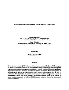
Figure 1: Density distribution of slope parameters (small threshold).

the searching could take a fair amount of time when the number of possible values is large. To reduce the computation load, we employ the method proposed by Hansen [17]. Specifically, instead of searching over all values of 𝑞𝑖𝑡 , we limit it to some specific quantiles {0.01, 0.0125, 0.015, . . . , 0.99}, which contain only 393 different values. However, this approach may not be as appealing as searching over all possible values of 𝛾 when the number of distinct value of 𝑞𝑖𝑡 is small. 4.2. Simulation Results. Tables 1 and 2 represent the 5%, 50%, and 95% quantiles of the simulation distribution of 𝛾̂, 𝛼̂1 , and 𝛼̂2 for 𝑇 varying among 10, 15, and 20 and 𝑁 varying among 100, 200, and 300. Table 1 reports the results of 𝜃 = 0.1, corresponding to the case when threshold is small. The estimates of the threshold 𝛾 perform fairly well for all cases considered, since the medians of 𝛾̂ are around the true value 𝛾 = 2. As 𝑇 increases, the distribution of 𝛾̂ is becoming more and more concentrated around the true value. For example, when 𝑁 = 100 and 𝑇 = 10, the length of the quantile range between 0.05

and 0.95 is 4.02, while, when 𝑇 = 20, the length decreases to 0.95. The distribution of the slope coefficient estimator 𝛼̂1 exhibits a little downward bias as it has been shown in some of the existing Monte Carlo studies for dynamic panel data models. For 𝑁 = 100 and 𝑇 = 10, the median bias of 𝛼̂1 is 0.06, but this bias is reduced as N and/or 𝑇 increases; for example, this bias is only 0.01 for 𝑁 = 300 and 𝑇 = 20. Similarly, the length of the quantile range between 0.05 and 0.95 for 𝛼̂1 is getting smaller as 𝑇 increases, which means that the performance improves. The quantiles of the distribution of 𝛼̂2 also performs well in all cases, although it is relatively weak in cases with small 𝑇 and small N. Table 2 presents the results for the case when threshold is big; that is, 𝜃 = 0.3. Compared to the small threshold case, the performance of the distribution of 𝛾̂ is improved. The median bias of 𝛾̂ is zero for almost all cases, and the length of the quantile range between 0.05 and 0.95 is getting smaller as the threshold effect increases. Meanwhile, Table 2 reports similar results as Table 1 for the parameters of 𝛼̂1 and 𝛼̂2 . In Table 2, they also perform fairly well in the big threshold case.

6

Mathematical Problems in Engineering 𝛼1 = 0.5, T = 10

10

12

12

4

Density

Density

Density

6

6 4

0.4

0.5

0.6

0 0.3

0.7

0.4

0.5

0 0.3

0.6

0.4 x = 0.5 N = 100

N = 200 N = 300

(b)

𝛼2 = 0.8, T = 10

12

𝛼2 = 0.8, T = 15

16

6 4

2

2

0 0.5

0 0.6

0.7

0.8

0.9

1

𝛼2 = 0.8, T = 20

12 Density

Density

4

10 8 6 4 2

0.7

0.8

0.9

0 0.6

0.7

x

x

N = 200 N = 300

N = 200 N = 300

14

8

6

0.6

(c)

10

8

0.5 x

x = 0.5 N = 100

N = 200 N = 300

(a)

x = 0.8 N = 100

6

x

x = 0.5 N = 100

0.6

8

2

x

10

10

4

2 0.3

𝛼1 = 0.5, T = 20

14

8

2

Density

16

10

8

0 0.2

𝛼1 = 0.5, T = 15

x = 0.8 N = 100

(d)

0.8

0.9

x

N = 200 N = 300

(e)

x = 0.8 N = 100

N = 200 N = 300

(f)

Figure 2: Density distribution of slope parameters (big threshold).

Figure 1 displays kernel estimates of the distribution of the slope parameters 𝛼̂1 and 𝛼̂2 based on 1,000 replications with 𝑁 = 100, 200, 300, 𝑇 = 10, 15, 20, and small threshold (𝜃 = 0.1). The estimates are slightly biased downwards when 𝑇 is small or 𝑁 is small. This bias is common in dynamic panel data model as mentioned earlier. One could also use some bias-corrected methods to improve the finite sample properties of the estimators, which is beyond the scope of this paper. The estimates are gradually centered around the true values as 𝑁 and/or 𝑇 increases, which is consistent with the above analyses and confirms the validity of our proposed estimation procedure again. Figure 2 shows the distribution of the same parameters as Figure 1 and based on the same number of replications and sample size but with bigger threshold (𝜃 = 0.3). In this case the same conclusion can be found as in Figure 1. In particular, the performance of the estimators in this case is better than that in the smaller threshold for all cases.

5. Conclusion This paper extends the estimation of threshold models in nondynamic panels to dynamic panels and presents practical estimation methods for these econometric models with individual-specific effects and threshold effects. The foremost feature of these models is that they allow the econometrician to consider the dynamic and threshold relationships in economic system simultaneously. As mentioned in the introduction, many applications may have such relationships. Using the first-difference to eliminate the individual-specific effects, we prove that the orthogonality conditions proposed by Arellano and Bond [10] for nonthreshold models are also valid in our models. Then, we estimate the threshold and slope parameters by GMM. Monte Carlo simulations reveal that our method has very good finite sample performance. There are several possible extensions to this work. The asymptotic properties of the threshold parameter would be

Mathematical Problems in Engineering an interesting topic. Also, testing for one or multiple thresholds is also worth studying, which is saved for future research.

Conflict of Interests The authors declare that there is no conflict of interests regarding the publication of this paper.

Acknowledgments The authors thank the editor and three anonymous referees for many constructive and helpful comments. This work was partially supported by the National Natural Science Foundation of China (Grant nos. 71301160 and 71301173), China Postdoctoral Science Foundation funded project (Grant nos. 2012M520419, 2012M520420, and 2013T60186), Beijing Planning Office of Philosophy and Social Science (13JGB018), and Program for Innovation Research in Central University of Finance and Economics.

References [1] C. X. Huang, C. L. Peng, X. H. Chen, and F. H. Wen, “Dynamics analysis of a class of delayed economic model,” Abstract and Applied Analysis, vol. 2013, Article ID 962738, 12 pages, 2013. [2] F. Wen and Z. Dai, “Modified Yabe-Takano nonlinear conjugate gradient method,” Pacific Journal of Optimization, vol. 8, no. 2, pp. 347–360, 2012. [3] O. Galor and D. N. Weil, “Population, technology, and growth: from malthusian stagnation to the demographic transition and beyond,” The American Economic Review, vol. 90, no. 4, pp. 806– 828, 2000. [4] A. Mas-colell and A. Razin, “A model of intersectioral migration and growth,” Oxford Economic Papers, vol. 25, no. 1, pp. 72–79, 1973. [5] P. F. Peretto, “Industrial development, technological change, and long-run growth,” Journal of Development Economics, vol. 59, no. 2, pp. 389–417, 1999. [6] T. W. Anderson and C. Hsiao, “Estimation of dynamic models with error components,” Journal of the American Statistical Association, vol. 76, no. 375, pp. 598–606, 1981. [7] A. Ciarreta and A. Zarraga, “Economic growth-electricity consumption causality in 12 European countries: a dynamic panel data approach,” Energy Policy, vol. 38, no. 7, pp. 3790– 3796, 2010. [8] T. S. Eicher and T. Schreiber, “Structural policies and growth: time series evidence from a natural experiment,” Journal of Development Economics, vol. 91, no. 1, pp. 169–179, 2010. [9] B.-N. Huang, M. J. Hwang, and C. W. Yang, “Causal relationship between energy consumption and GDP growth revisited: a dynamic panel data approach,” Ecological Economics, vol. 67, no. 1, pp. 41–54, 2008. [10] M. Arellano and S. Bond, “Some tests of specification for panel data: Monte Carlo evidence and an application to employment equations,” The Review of Economic Studies, vol. 58, pp. 277–297, 1991. [11] M. Arellano and O. Bover, “Another look at the instrumental variable estimation of error-components models,” Journal of Econometrics, vol. 68, no. 1, pp. 29–51, 1995.

7 [12] R. Blundell and S. Bond, “Initial conditions and moment restrictions in dynamic panel data models,” Journal of Econometrics, vol. 87, no. 1, pp. 115–143, 1998. [13] B. H. Baltagi, Econometric Analysis of Panel Data, John Wiley & Sons, Chichester, UK, 2008. [14] C. Han and P. C. B. Phillips, “GMM estimation for dynamic panels with fixed effects and strong instruments at unity,” Econometric Theory, vol. 26, no. 1, pp. 119–151, 2010. [15] B. E. Hansen, “Sample splitting and threshold estimation,” Econometrica, vol. 68, no. 3, pp. 575–603, 2000. [16] M. Caner and B. E. Hansen, “Instrumental variable estimation of a threshold model,” Econometric Theory, vol. 20, no. 5, pp. 813–843, 2004. [17] B. E. Hansen, “Threshold effects in non-dynamic panels: estimation, testing, and inference,” Journal of Econometrics, vol. 93, no. 2, pp. 345–368, 1999. [18] J. Cheng, C. Lin, and C. Wang, “Estimation of growth convergence using common correlated effects approaches,” Working Paper, 2009. [19] T. T. L. Chong, Q. He, and M. J. Hinich, “The nonlinear dynamics of foreign reserves and currency crises,” Studies in Nonlinear Dynamics & Econometrics, vol. 12, no. 4, article 2, 2008. [20] T.-W. Ho, “Income thresholds and growth convergence: a panel data approach,” Manchester School, vol. 74, no. 2, pp. 170–189, 2006. [21] S. Kremer, A. Bick, and D. Nautz, “Inflation and growth: new evidence from a dynamic panel threshold analysis,” Empirical Economics, vol. 44, pp. 861–878, 2013. [22] V. A. Dang, M. Kim, and Y. Shin, “Asymmetric capital structure adjustments: new evidence from dynamic panel threshold models,” Journal of Empirical Finance, vol. 19, no. 4, pp. 465– 482, 2012. [23] K. S. Chan, “Consistency and limiting distribution of the least squares estimator of a threshold autoregressive model,” The Annals of Statistics, vol. 21, no. 1, pp. 520–533, 1993. [24] L. P. Hansen, “Large sample properties of generalized method of moments estimators,” Econometrica, vol. 50, no. 4, pp. 1029– 1054, 1982. [25] F. Windmeijer, “A finite sample correction for the variance of linear efficient two-step GMM estimators,” Journal of Econometrics, vol. 126, no. 1, pp. 25–51, 2005.

Advances in

Operations Research Hindawi Publishing Corporation http://www.hindawi.com

Volume 2014

Advances in

Decision Sciences Hindawi Publishing Corporation http://www.hindawi.com

Volume 2014

Journal of

Applied Mathematics

Algebra

Hindawi Publishing Corporation http://www.hindawi.com

Hindawi Publishing Corporation http://www.hindawi.com

Volume 2014

Journal of

Probability and Statistics Volume 2014

The Scientific World Journal Hindawi Publishing Corporation http://www.hindawi.com

Hindawi Publishing Corporation http://www.hindawi.com

Volume 2014

International Journal of

Differential Equations Hindawi Publishing Corporation http://www.hindawi.com

Volume 2014

Volume 2014

Submit your manuscripts at http://www.hindawi.com International Journal of

Advances in

Combinatorics Hindawi Publishing Corporation http://www.hindawi.com

Mathematical Physics Hindawi Publishing Corporation http://www.hindawi.com

Volume 2014

Journal of

Complex Analysis Hindawi Publishing Corporation http://www.hindawi.com

Volume 2014

International Journal of Mathematics and Mathematical Sciences

Mathematical Problems in Engineering

Journal of

Mathematics Hindawi Publishing Corporation http://www.hindawi.com

Volume 2014

Hindawi Publishing Corporation http://www.hindawi.com

Volume 2014

Volume 2014

Hindawi Publishing Corporation http://www.hindawi.com

Volume 2014

Discrete Mathematics

Journal of

Volume 2014

Hindawi Publishing Corporation http://www.hindawi.com

Discrete Dynamics in Nature and Society

Journal of

Function Spaces Hindawi Publishing Corporation http://www.hindawi.com

Abstract and Applied Analysis

Volume 2014

Hindawi Publishing Corporation http://www.hindawi.com

Volume 2014

Hindawi Publishing Corporation http://www.hindawi.com

Volume 2014

International Journal of

Journal of

Stochastic Analysis

Optimization

Hindawi Publishing Corporation http://www.hindawi.com

Hindawi Publishing Corporation http://www.hindawi.com

Volume 2014

Volume 2014