ESTIMATION OF SPECTRAL PARAMETERS OF RESIDUAL ECG SIGNAL DURING ATRIAL FIBRILLATION USING AUTOREGRESSIVE MODELS. R. Sassi1, L.T. Mainardi2, P. Maison-Blanche3 and S. Cerutti2 1 Dip. di Tecnologie dell’Informazione, Università di Milano, via Bramante 65, 26013 Crema, Italy 2 Dipartimento di Bioingegneria, Politecnico di Milano, Via Golgi 39, 20133 Milano, Italy 3 Department of Cardiology, Lariboisière Hospital, Paris, France e-mail:
[email protected]
Abstract: The application of AutoRegressive (AR) models to extract spectral parameters from residual ECG (rECG) signals is exploited. In particular, a new method based on AR spectra is employed to estimate the dominant atrial cycle length (DACL) on ECG obtained from patients undergoing episodes of atrial fibrillation (AF). The traditional FFT-based spectral approach will be compared with the new method. Potentialities and possible superior performances of AR spectra are documented and discussed. INTRODUCTION: In the last two decades, spectral analysis of the residual ECG signal (rECG, i.e. an ECG signal in which ventricular components were canceled through beat averaging techniques) has been employed to characterize atrial activities. The method is particularly relevant during atrial fibrillation (AF), after infusion of drugs or when various abnormal atrial rhythms are present. Typically, for a patient undergoing AF, a main spectral component f0 is found in the range 3-12 Hz. The inverse of f0 (the so called Dominant Atrial Cycle Length, DACL) has been related to atrial refractoriness and therefore to the probability of AF-maintenance through atrial electrical remodeling [1]. Recently, different authors have observed an increase DACL before spontaneous termination of AF [2]. The same technique was successfully employed for the analysis of long-term Holter recordings: in this framework however, movement artifacts and external noises may become critical factors for a reliable spectral estimation. A step forward would be the development of techniques able to provide robust, automatic estimation of rECG spectral parameters in long-term Holter recordings. Commonly, non-parametric, FFT-based methods, like the Welch's averaged, modified periodogram method, are employed for DACL computation [3-
4]. Nevertheless, model-based spectral estimators have potential theoretical advantages when dealing with low-components, noisy signals. In addition, the use of a spectral-decomposition method [5] would provide a natural alternative for f0 estimate. In this paper, rECG were constructed for each recording in the spontaneous termination AF database available from PhysioNet. Power spectra of rECG were obtained with estimators based on AR models and FFT. The different f0 frequencies derived from the two approaches were then compared. METHOD: Atrial Fibrillation Database. We based our analysis on the 2004 PhysioNet/Computers in Cardiology Challenge Database. It includes a collection of 80 digitized two-channel ECG recordings. Each record is a one-minute segment of atrial fibrillation, sampled at 128 Hz. All the recordings therein were considered. Signal pre-processing. Extraction of the residual ECG was obtained through beat-to-beat subtractions of an averaged QRST complex [2-4]. Despite the dataset already contained QRS annotations, ventricular beats were mainly misclassified. Thus, QRS detection was performed using a modified version of OSEA [6], a freely available ECG library. QRS onsets and widths were further refined by means of a second publicly available software, ECGPUWAVE [7]. Then, on a lead-by-lead basis, separate average templates were built for QRS and T waves. Subtraction of the templates was performed after a warping procedure and subsequent templates were connected via linear interpolation. Spectral Estimation. The power spectral density (PSD) of rECG was firstly estimated using the Welch’s periodogram (512-points Kaiser’s
108
PSD / variance
(a)
(b)
0.2
0.2
0.18
0.18
0.16
0.16
0.14
0.14
0.12
0.12
0.1
0.1
0.08
0.08
0.06
0.06
0.04
0.04
0.02
0.02
0
0 0
10
20
30 Hz
40
50
60
0
10
20
30 Hz
40
50
60
Fig. 1. Power spectral densities of two different rECGs: recoding N01 lead 1 (a) and N03 lead 1 (b). The nonparametric spectrum (rough line), the parametric spectrum (thick line, M=8) and the SL component (dash-dot line) are superimposed. The smaller box in the upper right corner of each panel is a magnification of the area contained in the dotted box. The vertical dotted lines delimit the range 3-12 Hz. The markers show the position of the four estimates of f0: fNP (method M1, star), fL (method M2, cross), fC (method M3, black dot) and fP (method M4, circle). In panel (b), the black triangle marks the position of f0 as obtained from lead 2 in the same recording.
window with an overlap of 256 points). The technique ensured a spectral resolution of 0.25 Hz and a reasonably low variance of the PSD estimator (averaged over 29 windows). The non parametric spectrum was finally inspected for a peak in the range 3-12 Hz. The frequency fNP at which the peak maximum was occurring is the non-parametric estimate of f0 (method M1).
where γk is the residue relative to pole pk. Consequently the PSD can be separated into M contributions, relative to each pole:
Autoregressive Spectral Estimation. An autoregressive (AR) model
We considered three different parametric estimates of f0.: namely, fL (method M2), fC (method M3) and fP (method M4). A brief description of the way they were computed is reported below. Method M2: Firstly, we selected the pole pL in the range 312 Hz with the largest residue γL (thus the largest associated power). The frequency fL was given by f L = f S ϑ ( p L ) /(2π ) , where θ(x) is the phase (expressed in radiant) of the complex number x. Method M3: The pole pL, compute above, is associated with the PSD component SL(f). The frequency fC is the abscissa at which SL(f) reaches its maximum value. The value was obtained analytically, using a formula which is omitted here for compactness reasons. Method M4. Finally, we numerically located in the range 3-12 Hz the frequency fP at which the parametric PSD(f) reached its maximum. fP is the parametric equivalent of fNP.
M
y n = −∑i =1 ai y n−i + wn , where wn is a white Gaussian noise with zero mean and standard deviation σG, was fitted for each rECG series (covariance method). The rECG series were preliminarily down-sampled at fS=32 Hz to simplify the fitting procedure. We found empirically that M=8 was a reasonable value for the order of the AR model. Please refer to the concluding section for a discussion on this issue. The PSD for an AR process is given by
PSD( f ) =
σ G2 / f S M
1 + ∑k =1 a k e
− j 2πkf / f S
2
.
Using the Cauchy residue theorem, the total power of the rECG series, σ2rECG, can be decomposed [5] into M contributions, one for each pole of the AR model: M
2 σ rECG = σ G2 ∑k =1 γ k ,
M
PSD( f ) = ∑k =1 S k ( f ) , with:
Sk =
γ k (1 − pk2 ) 1 + p − 2 pk cos(2πf / f S ) 2 k
σ G2 / f S .
RESULTS: The power spectral densities of two different rECGs are shown in Fig. 1.
109
Error (Hz)
0.4 0.3 0.2 0.1 0.0 -0.1 -0.2 -0.3 -0.4 M1-M2
M1-M3
M1-M4
M2-M3
M2-M4
M3-M4
Algorithms
Figure 2. Mean (gray) and standard (black) errors of the differences between f0 estimates, as obtained from the two methods indicated in abscissa.
It is worth noting that The FFT- and AR-based spectra are in good agreement. In the case of panel (a) the four methods lead to very similar results. The advantages of the AR approach emerge when the intensity of the fibrillatory wave is rather small and not well concentrated in frequency, as in panel (b). In this case method M1 and M4 failed in providing a value of f0 which might be in agreement with the other ECG lead (where the spectral peak was clearly evident). We then tested if the different methods were able to provide consistent results. A comparison of the different approaches is shown in Fig. 2. All the techniques were in broad agreement among them. M2 and M3 provided the closest estimates of f0. The results obtained using M1 were also in close agreement with M2 and M3 but an average overestimation of DACL was observed. Conversely, method M4 showed the largest deviation from the other approaches. The database contained two-channel ECG recordings and a value of f0.was obtained from each lead. We tested if these two estimates were in agreement among them, for each of the four methods. Given that the estimates were correct, the main idea under this comparison was that the more the two estimates were close together the more a method was likely to be precise. We observed that M2 and M3 provided the smallest average differences among leads (M1: -0.234 ± 0.742 Hz, M2: -0.163 ± 0.409 Hz, M3: -0.158 ± 0.427 Hz, M4: -0.208 ± 0.824 Hz, please note that the spectral resolution of the FFT-based method was 0.25 Hz). But more significantly, the standard deviations of M2 and M3 were the smallest, suggesting a possible higher accuracy.
In the paper three parametric methods to estimate f0 were suggested. They proved to be in good agreement among them and with the classical FFT-based approach. In particular, M2 and M3 showed to be the most consistent among each other and they offered the smallest variation between estimates on different leads. Being M2 less computationally demanding, we selected it as our first choice method. M4 performed poorly, compared to the other three methods. This is related to the order of the model we selected (M=8). When M is small, the AR models extract the prevalent features of the rECG signals, among which the fibrillatory wave emerge clearly. In this situation, M2 and M3 excel. On the contrary, when M is very high, the parametric spectrum tends to be identical to the nonparametric one. Thus M1 and M4 lead to similar results, while M2 and M3 are penalized by overfitting effects. In this limit, the fibrillatory wave is buried among other details and the convenience of the AR approach over the classical one vanishes. We numerically verified that values of M between 7 and 10 offered the best compromise among these two limits. References: 1. Slocum J, Sahakian A, Swiryn S. Diagnosis of
2.
3.
4.
5.
6. CONCLUSIONS:
atrial fibrillation from surface electrocardiograms based on computer-detected atrial activity. J Electrocardiol. 1992;25:1-8. Mainardi LT, Matteucci M, Sassi R. On predicting the spontaneous termination of Atrial fibrillation episodes using linear and non-linear parameters of ECG signal and RR series, Proc. of CinC Conf. Chicago 2004, 665-669. Holm M, Pehrson S, Ingemansson M, Sornmo L, Johansson R, Sandhall L, Sunemark M, Smideberg B, Olsson C and Olsson SB. Non-invasive assessment of the atrial cycle length during atrial fibrillation in man: introducing, validating and illustrating a new ECG method. Cardiovascular Research 1998;38:69-81. J. Slocum, A. Sahakian and S. Swiryn. Diagnosis of Atrial Fibrillation From Surface Electrocardiograms Based on Computer-detected Atrial Activity. J Electrocardiol 1992;25(1):1-8. Baselli G, et al.Spectral Decomposition in Multichannel Recordings Based on Multivariate Parametric Identification. IEEE Trans. Biomed. Eng. 1997; 44:1092–1101. Hamilton P, Open Source ECG Analysis Software, EP Limited, www.eplimited.com
7. Laguna P, Jané R, Bogatell E, Anglada DV. ECGPUWAVE, www.physionet.org.
110