Estimation of Staphylococcus aureus Growth Parameters from ...

APPLIED AND ENVIRONMENTAL MICROBIOLOGY, July 2006, p. 4862–4870 0099-2240/06/$08.00⫹0 doi:10.1128/AEM.00251-06 Copyright © 2006, American Society for Microbiology. All Rights Reserved.

Vol. 72, No. 7

Estimation of Staphylococcus aureus Growth Parameters from Turbidity Data: Characterization of Strain Variation and Comparison of Methods R. Lindqvist* Microbiology Division, Department of Research and Development, National Food Administration, Uppsala, Sweden Received 1 February 2006/Accepted 9 May 2006

Turbidity methods offer possibilities for generating data required for addressing microorganism variability in risk modeling given that the results of these methods correspond to those of viable count methods. The objectives of this study were to identify the best approach for determining growth parameters based on turbidity data and use of a Bioscreen instrument and to characterize variability in growth parameters of 34 Staphylococcus aureus strains of different biotypes isolated from broiler carcasses. Growth parameters were estimated by fitting primary growth models to turbidity growth curves or to detection times of serially diluted cultures either directly or by using an analysis of variance (ANOVA) approach. The maximum specific growth rates in chicken broth at 17°C estimated by time to detection methods were in good agreement with viable count estimates, whereas growth models (exponential and Richards) underestimated growth rates. Time to detection methods were selected for strain characterization. The variation of growth parameters among strains was best described by either the logistic or lognormal distribution, but definitive conclusions require a larger data set. The distribution of the physiological state parameter ranged from 0.01 to 0.92 and was not significantly different from a normal distribution. Strain variability was important, and the coefficient of variation of growth parameters was up to six times larger among strains than within strains. It is suggested to apply a time to detection (ANOVA) approach using turbidity measurements for convenient and accurate estimation of growth parameters. The results emphasize the need to consider implications of strain variability for predictive modeling and risk assessment. commonly measured as the absorbance of light of a defined wavelength (19). A specific area of concern is the relation between what is measured, absorbance, and bacterial numbers and the constancy of this relation over the duration of the experiment. In some studies, absorbance data are used directly, whereas in others, efforts are made to establish calibration curves by defining the relationship between the absorbance and bacterial counts (17). Several approaches to estimate growth parameters from turbidity data exist, and these have recently been described and compared (10). In general, the approaches are based either on fitting primary growth equations to absorbance data directly, to log-transformed data, or to detection times of serially diluted cultures. One advantage of the latter approach is that a calibration between absorbance and numbers is not necessary (the Baranyi-Pin [BP] method described below), or an initial single measurement is sufficient (decimal dilution [DD] method described below). Dalgaard and Koutsoumanis (10) concluded that accurate estimates based on absorbance data were obtained from fitting a Richards model with fixed values for m, a parameter describing the degree of dampening in growth, as well as from absorbance detection times of serially diluted cultures. The ␮max values estimated with these models were independent of the growth yield, in contrast to ␮max values estimated with, for instance, the exponential growth model. It was suggested that the Richards and time to detection methods were complementary and would best be used together (10). One of the time to detection approaches is based on the Baranyi growth model and employs an analysis of variance (ANOVA) procedure as suggested by Baranyi and Pin (2) to estimate the specific growth rate and the physiological state variable. The lag time can be derived from these parameters.

Quantitative risk assessments increasingly form the basis for risk management decisions concerning food-borne microbial hazards (15). An important step in the assessments is the use of predictive models to describe microbial responses, such as growth, survival, and inactivation, in order to calculate exposure (20, 27). Apart from accurate estimation of single model parameter values, such as the maximum specific growth rate (␮max) and lag time (␭), it is also desirable to have information on the distributions of the parameter values, since a deterministic approach not taking strain variability into account may provide an incomplete or misleading result (21, 31). The literature on strain variation and of the characteristics of the parameter distributions is still rather meager (33). One reason for this gap in knowledge is the appreciable work required to obtain these data. The increased need for accurate data is difficult to meet with the use of the classic viable count methods (17). In this respect, automated optical measurement methods can be useful but need to be evaluated against the classic methods. Estimation of microbial growth parameters from measurements of turbidity has the advantages of being rapid, nondestructive, and relatively inexpensive compared to many other techniques, e.g., classical viable count methods (10). However, turbidity methods also have limitations, such as being applicable only to liquid cultures and having high detection limits in the range of 106 to 107 bacteria ml⫺1 and consequently yielding little direct information on the lag phase. The turbidity of a suspension is * Corresponding author. Mailing address: Microbiology Division, Department of Research and Development, National Food Administration, P.O. Box 622, SE-751 26 Uppsala, Sweden. Phone: 46 18 175631. Fax: 46 18 105848. E-mail: [email protected]. 4862

VOL. 72, 2006

GROWTH PARAMETER ESTIMATIONS

The physiological state parameter is a dimensionless parameter quantifying the suitability of the culture to the actual environment. The extreme values of the parameter are 0 and 1, and the values correspond to situations where the growth curve has an infinitely long lag time and no lag, respectively (2). The authors estimated the parameter values for a cocktail of three Pseudomonas species but did not present results that compared the estimates with values estimated from viable count data. In the study by Dalgaard and Koutsoumanis (10), summary results from experiments using a lower number of replications of serially diluted cultures than in the original study by Baranyi and Pin (2) and mixtures of five to eight strains of a range of species (not Staphylococcus aureus) were presented. The results suggested that the ANOVA procedure (2) yielded accurate estimates of ␮max values as indicated by the mean ratio of the ␮max determined by viable counts to the ␮max determined by the ANOVA procedure of 0.97 ⫾ 0.16 (standard deviation). Conclusions on the importance of strain-to-strain variation for predictive models vary, possibly reflecting the conditions and strains used in the different studies. Oscar (23) reported that the coefficient of variation (CV) for growth rates were similar among and within individual Salmonella strains growing in sterile ground chicken breast burgers at 25°C. In contrast, Begot et al. (6) found strain variation more important when investigating the growth response of 66 Listeria monocytogenes and Listeria innocua strains of variable origin under different growth conditions. The authors did not report the coefficients of variation, but the differences between minimum and maximum parameter values among strains were greatest for estimated lag times, 25 times, whereas the maximum variation in generation times, and thus growth rates, was two to three times. An extensive strain-to-strain variation in growth rates was also reported for strains of L. monocytogenes belonging to three different genotypic lineages (11). Similarly, the importance of variation among strains of Escherichia coli O157:H7 was concluded, since the coefficients of variation of estimated growth parameters among 17 strains were larger than those assessed from experiments using single strains (33). Dengremont and Membre´ (13) employed multivariate data analysis to identify three groups among five Staphylococcus aureus strains using growth rates at different combinations of temperatures, pHs, and NaCl concentrations as the identification characteristic. The overall objectives of this study were twofold: (i) to identify the best approach, in terms of accuracy and convenience, for determining growth parameters using turbidity data; and (ii) to apply this approach to the characterization of the variation in growth parameters of Staphylococcus aureus strains isolated from Swedish chicken carcasses. Specifically, three approaches for determining growth parameters by means of detection times (2, 10) and two approaches by fitting growth models to turbidity growth curves directly (10) were validated against viable count data. MATERIALS AND METHODS Bacteria and culture conditions. In a baseline study carried out from September 2002 to August 2003, 636 broiler chickens slaughtered at the 10 largest slaughterhouses in Sweden were sampled at the end of the slaughter process and examined for the presence of several bacteria. From two thirds of the chicken carcasses, coagulase-positive staphylococci were isolated. About 100 of these

4863

strains were selected for further characterization by classification to the species level based on aerobic growth on maltose purple agar plates by the method of Kloos and Schleifer (18) and to the biotype level by the method of Devriese (14). Of these, 34 isolates representing three different biotypes (poultry, non-hostspecific [NHS], and unclassified biotypes) were selected for inclusion in this study (see Table 4). The uniqueness of the strains was not confirmed by any genetic typing method, but selected strains were isolated from broilers slaughtered on different days. Two of the strains, S30 (poultry) and S119 (NHS), were used in the experiments for evaluating the different methods for determination of growth parameters. Growth parameters were determined from turbidity data using five different methods and compared with parameters determined from viable count data. The experimental culture conditions were selected to simulate the growth conditions in temperature-abused cooked chicken meat. Experiments were performed at 17°C in a broth simulating the reported properties of a cooked cured chicken meat product (8), chicken broth. The chicken broth was prepared using brain heart infusion (BHI) broth (Difco) as a base with pH, water activity (aw), and concentrations of salts adjusted to the values reported previously (8). To achieve the desired aw, glycerol was used in addition to NaCl as a humectant. To the dissolved BHI broth, 7.14% glycerol and a concentration of 1.76% NaCl and 39 ppm NaNO2 was added to get a final aw of 0.971. The pH value was set to 6.3 with HCl. The final pH (PHM 210 pH-meter; MeterLab Instruments, Radiometer, Denmark) and aw (AquaLab series 3TE; Decagon Devices, Inc., WA) were checked after the medium had been autoclaved. Strains were stored at ⫺70°C in BHI broth with 20% glycerol. Prior to an experiment, strains were inoculated on blood agar plates (Oxoid, England) and incubated for 24 h at 37°C. One colony from each isolate was inoculated in tubes with 5 ml chicken broth and grown overnight (18 to 24 h) at 37°C. A 0.1-ml volume of the culture was transferred into a new tube and grown overnight as described above. This was repeated once more, before the appropriate dilutions of the culture suspension were used in the experiments. Growth measurements. In order to identify the best approach to estimate growth parameters, the growth of two strains, S30 and S119, was quantified by viable count data and compared with growth estimated from five methods based on turbidity measurements. The turbidity of the bacterial suspensions was measured as the absorbance at 420 to 580 nm using the wideband filter in the Bioscreen C instrument, an automated turbidity reader (Oy Growth Curves AB Ltd., Helsinki, Finland). The turbidity methods evaluated were the exponential growth and Richards methods, which were based on turbidity growth curves, and the decimal dilution (DD), Baranyi-Pin decimal dilution (BPdec), and BaranyiPin binary dilution (BPbin) methods, which were based on the time to the detection of turbidity in serially diluted cultures (see below). For all methods, strains were cultured as described above. The procedure for preparing bacterial suspensions of the desired concentration was standardized by adjusting the turbidity of the initial stock suspensions, from which dilutions were made, to approximately 0.24 absorbance unit. This value was 0.03 unit or more above the turbidity of the sterile medium, the minimum difference used in reference 2, and represents the turbidity detection level. This turbidity corresponds to approximately 107 CFU ml⫺1. For the viable count method, the initial suspension was diluted to approximately 103 CFU ml⫺1. From this dilution, 300 ␮l was transferred to each one of the 30 wells in the Bioscreen microplate and incubated at 17°C for up to 8 days. At appropriate intervals, samples were withdrawn from wells in the microplate without removing it from the instrument, diluted in peptone water, and plated on Trypticase soy agar (Acumedia, Baltimore, MD) using a spiral plater (Eddy Jet; IUL Instruments, Germany). After incubation at 37°C for 24 h, the plates were read. Growth rate determination was done in duplicate wells in two replicate experiments. Blank sample wells with uninoculated broth were included as a control for contamination. Turbidity growth curves at 17°C were generated using the Bioscreen C instrument. Growth was followed by measuring the turbidity every 15 to 30 min for up to 12 days in wells inoculated with 300 ␮l bacterial suspensions of an initial concentration of approximately 104 CFU ml⫺1. The microplates were shaken for 5 seconds prior to measurement of turbidity. Growth rate determination was done in triplicate wells in three replicate experiments. The time to detection experiments were carried out on duplicate wells of five consecutively decimally diluted cultures (DD and BPdec methods) or quadruplicate wells of five consecutively binary diluted cultures (BPbin method). Dilutions were prepared from stock suspensions with a turbidity just above the detection limit of the instrument as described above. The resulting initial bacterial concentrations for the different dilutions in the time to detection experiments were approximately 102 to 106 CFU ml⫺1 (DD and BPdec) and 3 ⫻ 102 to 0.5 ⫻ 104 (104/25 to 104/21) CFU ml⫺1 (BPbin), respectively. These experiments were re-

4864

LINDQVIST

APPL. ENVIRON. MICROBIOL.

peated two (BPbin) or three times. The time to detection methods DD and BPdec were selected for the characterization of strain variability in growth parameters, because ␮max values estimated by these methods were closer to viable count estimates than values estimated by growth curve methods, and for practical reasons, since both can be used with the same experimental setup (dilutions) in contrast to BPbin. For the different strains, the turbidity detection level corresponded to viable counts between 0.2 ⫻ 107 and 4.2 ⫻ 107 CFU ml⫺1. To illustrate this variation among strains, the initial number of cells per turbidity unit was calculated by dividing the turbidity in the initial suspension by the bacterial count (see Table 4). Growth parameters. The maximum specific growth rate ␮max and lag time ␭ were estimated from the viable count data by the Baranyi model (3) using the MicroFit software (version 1.0; Institute of Food Research, Norwich, United Kingdom [http://www.ifr.ac.uk/microfit/]). As described by Dalgaard and Koutsoumanis (10), ␮max values of the exponential growth model (equation 1) and the Richards model (equation 2) were estimated by regression analysis of turbidity growth curves. The LAB Fit Curve Fitting software (version 7.2.32; W. Pereira da Silva and C. Pereira da Silva [http://www.labfit.net]) was applied for the nonlinear regression analysis involved in estimating the parameters of the Richards model, and m in equation 2 was fixed to 0.5, 1, or 2. In addition, ␮max values were estimated from turbidity detection times of serially diluted cultures. The simplified approach (DD method, equation 3) described by Dalgaard and Koutsoumanis (10) to the decimal dilution method suggested by Cuppers and Smelt (9) and the ANOVA method (BPdec and BPbin, equations 4 and 5) of Baranyi and Pin (2) were used. In the DD method, the detection times of the serial dilutions were plotted against the natural logarithm of their initial bacterial counts, and ␮max and k2 were determined by linear regression according to equation 3. In the ANOVA method, a Microsoft Excel spreadsheet and Solver add-in was used to find the ␮max value that minimized the ratio of the summed between- and within-dilution variances of the physiological state variable ␣ (2). In this approach, both ␮max and the physiological state variable ␣ are estimated, and from these estimates, the lag time is calculated from equation 6 (2). Lag times were estimated with the DD method from equation 7 using the values of ␮max and k2 estimated from equation 3. ln(TURt) ⫽ k1 ⫹ ␮EXP · t TURt ⫽ TURmin ⫹

TURmax ⫺ TURmin (1 ⫹ e⫺␮Richards · m · (t ⫺ ti))1/m

ln(Nj) ⫽ k2 ⫺ ␮DD · Tj ␣j ⫽

rj ⫽

e

(2) (3)

⫺␮Tj

rj Nj Xdet

␭BP ⫽ ⫺

␭DD ⫽

(1)

ln␣ ␮BP

k2 ⫺ ln共Xdet兲 ␮DD

(4)

(5)

(6)

(7)

TUR is turbidity, and the subscripts t, min, and max refer to turbidity at time t and minimum and maximum turbidity, respectively. The maximum specific growth rate is ␮, and the lag time is ␭. The subscripts EXP, Richards, DD, and BP refer to the method used for growth parameter estimation, and k1 and k2 are constants (intercepts). In the Richards model, m is a shape parameter and ti is the time at the inflection point. Nj, Tj, rj, and ␣j indicate initial cell levels, turbidity detection times, dilution ratios, and physiological state parameters corresponding to different serially diluted cultures, respectively. Xdet is the bacterial count at the turbidity detection level. The ratio R between the ␮max values estimated from viable count (indicated by subscript vc) and the different turbidity methods (indicated by subscript Exp, R, DD, or BP) was calculated as ␮vc/␮ of the turbidity method for each method. In the same way, the ratio R was estimated for ␭ values. The apparent growth yield of strains was expressed as the mean difference between the initial and final turbidity measurements in the detection time experiments. Nonlinearity of turbidity response was not corrected for. The 10- and 100-fold dilutions of the cultures were used, since there was no significant

difference in the apparent growth yield between these dilutions as opposed to higher dilutions. Statistical and distribution analyses. Analysis of variance was used to examine for possible effects of the method and biotype on the estimates of growth parameters. For each method, a two-sample t test was carried out to test whether the mean growth rate and mean lag time estimated by the method differed from the parameters estimated by the viable count method. This analysis was not possible for the lag time of strain S30, since only one observation of lag time based on viable counts was available. To test whether the correlation between apparent growth yield and estimated growth parameters was different from zero, Pearson product-moment correlation coefficients were calculated. The statistical tests above were performed with Minitab version 12.22 (Minitab Inc., State College, PA), and in the ANOVA, a generalized linear model, GLM, with no interactions between factors was used. The growth parameter values estimated from the growth experiments of the 34 strains were used to determine the distributions of growth parameters among strains. The Kolmogorov-Smirnov (KS) test was used to test whether the growth parameters were normally distributed. The normal, lognormal, logistic, gamma, and Weibull distributions were fit to the growth rate, lag time, and physiological state data by the @Risk software package (version 4.0.5; Palisade Corporation, Newfield, N.Y.), and fitted distributions were ranked on the basis of the Kolmogorov-Smirnov test in combination with the Anderson-Darling (AD) test. A description of the distributions and their parameters can be found in reference 32. The coefficient of variation of growth parameters was calculated as the standard deviation divided by the mean and was compared to the CV for single strains (S30 and S119, respectively) to investigate the importance of strain variation. To evaluate whether the negative lag times estimated by the DD method were associated with poor fits of equation 3 to data, the effect of the sign of the lag time on the median R2 value was examined by the Mann-Whitney test.

RESULTS Evaluation of turbidity methods for determination of growth parameters. For both strains (S30 and S119), there was a highly significant effect of the method used for determining ␮max (ANOVA, P ⬍ 0.001) (Table 1). The maximum specific growth rates, ␮max, for strains S30 and S119 as determined by viable count methods were 0.13 and 0.16 h⫺1, respectively (Table 1). The mean ␮max values estimated by the turbidity methods ranged from 0.02 to 0.18 h⫺1 for strain S30 and from 0.02 to 0.13 h⫺1 for strain S119 (Table 1). The turbidity growth curve methods yielded smaller ␮max values than the time to detection methods. For both strains, the ␮max values estimated by the exponential growth model and Richards methods were lower and significantly different from the ␮max values estimated by viable count methods (t test, P ⬍ 0.001). In comparison, ␮max values estimated by the detection time methods were more similar to the viable count estimates. A statistically significant difference (t test, P ⬍ 0.05) when present was only observed for one of the two strains (Table 1). Average R␮ values, the ratio between ␮max values estimated by the viable count method and the respective turbidity methods, i.e., the correction factors, ranged from 0.98 (BPbin) to 7.25 (exponential growth model) (Table 2). Lag times were estimated by the viable count and time to detection methods, but not by turbidity growth methods. There was no significant effect of methods in the estimation of lag times (ANOVA, P ⬎ 0.05). The mean lag times ranged from 8.8 to 19.5 h for strain S30 and from 12.2 to 28.7 h for strain S119 (Table 1). Average R␭ values, the ratio between ␭ values estimated by the viable count method and the respective time to detection method, ranged from 1.36 (BPdec) to 1.50 (BPbin) (Table 2). The coefficients of variation for determination of growth parameters of strains S30 and S119 were estimated from the

VOL. 72, 2006

GROWTH PARAMETER ESTIMATIONS

TABLE 1. Comparison of estimated maximum specific growth rates and lag times, determined by viable count and turbidity measurement methods for two strains of S. aureus Method and expt no. or parameter

␮max (h⫺1)a S30

TABLE 2. R, the ratio between ␮max and ␭ values determined by the viable count method and each turbidity method R for ␮max

␭ (h) S119

S30

0.140 0.120 0.13 (0.014)

0.170 0.150 0.16 (0.014)

Exponential Expt 1 Expt 1 Expt 1 Expt 2 Expt 2 Expt 2 Expt 3 Expt 3 Expt 3 Mean (SD)

0.014 0.016 0.016 0.024 0.025 0.023 0.028 0.013 0.015 0.02*** (0.006)

0.016 0.018 0.017 0.014 0.021 0.015 0.021 0.029 0.022 0.02*** (0.005)

ND ND ND ND ND ND ND ND ND

Richards Expt 1 Expt 1 Expt 1 Expt 2 Expt 2 Expt 2 Expt 3 Expt 3 Expt 3 Mean (SD)

0.095 0.091 0.093 0.058 0.060 0.060 0.062 0.064 0.065 0.07** (0.016)

0.066 0.059 0.070 0.071 0.070 0.092 0.067 0.063 0.074 0.07*** (0.009)

ND ND ND ND ND ND ND ND ND

ND ND ND ND ND ND ND ND ND

DD Expt 1 Expt 2 Expt 3 Mean (SD)

0.118 0.135 0.141 0.13 (0.012)

0.114 0.096 0.109 0.11* (0.009)

4.4 11.1 11.0 8.8 (4.7)

11.4 21.3 25.2 19.3 (7.1)

BPdec Expt 1 Expt 2 Expt 3 Mean (SD)

0.143 0.142 0.140 0.14 (0.001)

0.129 0.114 0.098 0.11* (0.015)

11.5 14.1 10.7 12.1 (1.8)

17.4 14.8 20.0 17.4 (2.6)

BPbin Expt 1 Expt 2 Mean (SD)

0.161 0.200 0.18 (0.028)

0.124 0.131 0.13 (0.005)

17.2 21.9 19.5 (3.4)

14.6 9.9 12.2 (3.3)

12.9 NDc 12.9b

R for ␭

S30

S119

Avg R␮ (correction factor)

S30

S119

Avg R␭ (correction factor)

Method S119

Viable count Expt 1 Expt 2 Mean (SD)

4865

24.4 32.9 28.7 (6.0)

Growth curve methods Exponential Richards

6.50 1.86

8.00 2.29

7.25 2.08

NDa ND

ND ND

ND ND

ND ND ND ND ND ND ND ND ND

Detection time methods BPdec BPbin DD

0.92 0.72 1.00

1.45 1.23 1.45

1.18 0.98 1.22

1.07 0.66 1.47

1.65 2.33 1.49

1.36 1.50 1.48

a Asterisks indicate that the mean of the parameter differs significantly (t test) from the parameter value determined for the same strain by the viable count method as follows: *, P ⬍ 0.05; **, P ⬍ 0.01; ***, P ⬍ 0.001. b Based on only one experiment and consequently comparisons with mean lag times determined for strain S30 by other methods were not done. c ND, not determined.

means and standard deviations of the repeated experiments and give an indication of the magnitude of stochastic variation associated with the current experimental conditions and methods (Table 3). In general, the mean CV was larger for the estimation of lag time than for ␮max values. For both the DD and BPdec methods selected for characterization of strains, the mean CV of ␮max was 0.08, which is similar to the CV of the viable count method (0.10) (Table 3). For lag time, the corresponding CV was 0.45 (DD) and 0.15 (BPdec) compared to 0.21, the CV of the viable count method (Table 3). Characterization of variation in the growth parameters of S. aureus strains. The ␮max, ␭, and ␣ values for the examined S. aureus strains are summarized in Table 4. The ␮max values of the strains as determined by BPdec ranged from 0.07 to

a

ND, not determined.

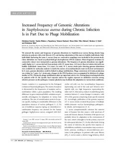
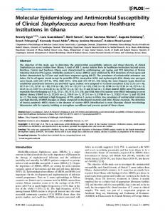
0.24 h⫺1 (corresponding to generation times of 2.9 to 9.9 h) and by DD from 0.04 to 0.26 h⫺1 (corresponding to generation times of 2.7 to 17.3 h). The lag times determined by the BPdec method ranged from 1.2 to 25.2 h. The lag times determined by the DD method were similar when positive, but for 10 strains, the estimation resulted in negative lag times. Negative lag times appeared to be associated with poor fits to the data, as suggested by significantly lower median R2 values in these experiments compared to experiments with positive lag times, 0.80 and 0.95, respectively (Mann-Whitney, P ⬍ 0.001). The BPdec method also yielded values of ␣, the physiological state parameter, ranging from 0.01 to 0.92. The mean ␮max value of the 34 strains estimated with the DD method was significantly lower than that with the BPdec method (t test, P ⬍ 0.01) (Table 4). There was no significant effect of strain biotype on mean ␮max, mean ␭, or mean ␣ as determined by the methods (ANOVA, P ⬎ 0.05). The distribution of ␣ as determined by BPdec and ␮max by the DD method was not significantly different from a normal distribution (KS, P ⬎ 0.15). In contrast, ␮max and ␭ determined by BPdec and ␭ determined by DD were significantly different from a normal distribution (KS, P ⬍ 0.05). The distribution of ␮max (BPdec) was best described by the logistic distribution, and the distribution of ␭ (BPdec) was best described by the lognormal distribution as ranked by the AD and KS tests (Fig. 1). For ␣ and ␮max (DD), the best distribution was either the logistic (KS) or lognormal (AD) distribution. However, for all parameters, the

TABLE 3. Coefficient of variation for determination of the maximum specific growth rate and lag time by viable count and turbidity methodsa CV of ␮max

Method S30

Viable count Exponential Richards BPdec Bpbin DD a b

0.11 0.30 0.23 0.01 0.16 0.09

S119

0.09 0.25 0.13 0.14 0.04 0.08

CV of ␭ Mean

0.10 0.28 0.18 0.08 0.10 0.08

S30 b

ND ND ND 0.15 0.17 0.53

S119

Mean

0.21 ND ND 0.15 0.27 0.37

0.21 ND ND 0.15 0.22 0.45

CVs were estimated from the mean and SD values in Table 1. ND, not determined.

4866

LINDQVIST

APPL. ENVIRON. MICROBIOL.

TABLE 4. Summary of the estimated growth parameters obtained by the BPdec and DD methods when the growth of 34 S. aureus strains of three different biotypes isolated from chicken carcasses were analyzed Biotype and strain or parameter

␣

␮ (h⫺1)

␭ (h)

␮ (h⫺1)

NHS S3 S4 S37 S57 S70 S87 S119 S126 S170 S192 S218 S272 S288 S312 S320 S347 S349 S361 S376 S395 Mean (SD)

0.51 0.02 0.72 0.92 0.33 0.12 0.14 0.38 0.22 0.10 0.43 0.46 0.25 0.50 0.01 0.40 0.13 0.63 0.42 0.26 0.35 (0.24)

0.09 0.22 0.08 0.07 0.14 0.15 0.10 0.18 0.12 0.13 0.08 0.09 0.15 0.09 0.19 0.10 0.13 0.09 0.12 0.13 0.12 (0.04)

7.3 18.2 3.9 1.2 7.8 14.2 20.0 5.4 13.3 18.0 10.9 8.8 9.5 7.7 25.2 9.0 15.9 5.1 7.1 10.6 10.9 (6.1)

Poultry S30 S39 S44 S54 S71 S111 S139 S286 S306 S344 S360 Mean (SD)

0.22 0.35 0.29 0.24 0.14 0.28 0.38 0.32 0.16 0.26 0.34 0.27 (0.08)

0.14 0.14 0.12 0.13 0.13 0.24 0.14 0.14 0.13 0.14 0.12 0.14 (0.03)

Unclassified S265 S293 S313 Mean (SD)

0.35 0.28 0.55 0.39 (0.14)

All strains Mean SD CV 95% CIb

0.33 0.19 0.58 0.26–0.39

a b

␭ (h)

Initial no. of cells per turbidity unit (108)

Apparent growth yield (turbidity units)

0.07 0.14 0.08 0.06 0.11 0.13 0.11 0.18 0.06 0.14 0.04 0.07 0.16 0.09 0.14 0.11 0.15 0.10 0.11 0.11 0.11 (0.04)

7.7 14.8 1.7 0.9 ⫺1.1 6.8 25.5 5.3 ⫺3.7 22.0 ⫺11.4 ⫺1.5 12.3 14.5 24.5 17.0 22.7 12.9 6.3 7.3 9.2 (10.2)

5.37 4.14 0.42 5.96 0.79 0.29 0.59 6.40 6.45 0.30 6.08 7.53 3.42 5.33 1.68 6.29 5.77 5.87 3.78 5.90 5.25 (0.93)

0.71 0.65 0.84 0.61 0.86 0.89 0.91 0.55 0.61 0.85 0.64 0.43 0.59 0.63 0.91 0.58 0.63 0.61 0.67 0.39 0.56 (0.11)

10.7 7.3 10.2 10.7 14.8 5.3 6.9 8.4 13.8 9.6 8.8 9.7 (2.8)

0.14 0.15 0.07 0.07 0.06 0.26 0.16 0.09 0.05 0.04 0.09 0.11 (0.06)

10.1 8.1 ⫺20.7 ⫺24.8 ⫺40.4 6.3 19.4 ⫺12.4 ⫺59.4 ⫺80.2 21.7 ⫺15.7 (33.4)

0.48 5.36 3.10 0.46 NDa 4.19 4.67 2.65 3.62 4.75 0.33 1.41 (2.16)

0.91 0.69 0.63 0.93 0.38 0.60 0.48 0.90 0.43 0.50 0.93 0.85 (0.14)

0.12 0.08 0.13 0.11 (0.02)

8.6 15.2 4.6 9.5 (5.4)

0.13 0.08 0.12 0.11 (0.02)

11.5 21.6 3.3 12.1 (9.2)

4.76 5.46 4.10 3.69 (0.55)

0.42 0.42 0.69 0.63 (0.04)

0.13 0.04 0.31 0.12–0.14

10.4 5.1 0.49 8.6–12.2

0.11 0.05 0.45 0.09–0.12

3.82 2.27 0.59 ND

0.66 0.18 0.27 ND

DD

BPdec

1.4 23.4 16.7 ⫺6.7–9.6

ND, not determined. For a normal distribution.

differences in the calculated test values of the AD and KS tests between the investigated distributions were small. The apparent growth yield expressed as the difference between the initial and final turbidity measurements of the cultures ranged from 0.38 to 0.93 turbidity unit (Table 4), and there was a significant difference in yield between biotypes (ANOVA, P ⬍ 0.001). This effect may not be real but a consequence of the use of apparent growth yield. This explanation is supported by the observation that the mean initial number of cells per turbidity unit was smallest for strains belonging to the biotype with the largest mean apparent yield (poultry) than for

the other biotypes (Table 4). There was a significant correlation between apparent growth yield and ␭ values determined by the DD method (correlation analysis, P ⬍ 0.01) but not for ␮max, or ␭, ␣, and ␮max determined by the BPdec method (correlation analysis, P ⬎ 0.15). DISCUSSION The time to detection methods were found to yield growth rates closer to viable count estimates than the growth curve methods. The good performance of these methods is in agree-

VOL. 72, 2006

GROWTH PARAMETER ESTIMATIONS

4867

FIG. 1. Distributions of estimated growth parameters among 34 S. aureus strains grown in chicken broth at 17°C. The circles represent observed data, and the lines show the best-fitting distribution functions as ranked by the Anderson-Darling test. a) Maximum specific growth rate, ␮max, estimated by the BPdec method, logistic distribution (0.125088; 0.019735) (the two values separated by semicolons are the parameter values for the distribution [␣ and ␤, respectively, for the logistic distribution and ␮ and ␴, respectively, for the lognormal distribution]); b) lag time, ␭, estimated by the BPdec method, lognormal distribution (17.318; 4.9808) ⫺6.9082 (the value outside the parentheses is the shift factor supplied by the BestFit software program if the input data exceed the domain range of the fitted distribution; the negative sign of the shift value indicates that this amount should be subtracted from the value drawn from the distribution); c) the physiological state variable, ␣ (BPdec), lognormal distribution (0.66041; 0.19039) ⫺0.33366; d) ␮max estimated by the DD method, lognormal distribution (0.12855; 0.046388) ⫺0.020530. The distributions and their parameters have been described by Vose (32).

ment with the results of Dalgaard and Koutsoumanis (10). In contrast to the present results, they obtained equally good results with one of the growth curve methods, the Richards method. Growth parameters estimated from turbidity and viable count data are more often than not unequal (1), and several potential sources of bias may contribute to these differences, e.g., turbidity detection limits in the range of declining growth rates (10), nonlinear relationships between absorbance and bacterial concentrations (19), and the selected growth model (5). For approaches based on the time to detection of turbidity, the first two sources of biases are less likely to interfere than for turbidity growth curve approaches that follow growth to a higher concentration. Absorbance becomes lower than that predicted from the Beer-Lambert law as the bacterial concentration increases, at an absorbance of 0.3 when light of 500 nm or shorter is used (19). Calibration curves relating absorbance to cell counts have also been reported to vary with increasing stress levels (17), and changes in cell viability (17) and cell morphology (26) have been suggested to contribute to this variation. In addition, different turbidity growth models differ in how much growth rate estimates are

influenced by these limitations as illustrated by the poor performance of the exponential model (the present study and reference 10). In the study by Dalgaard and Koutsoumanis (10), the use of turbidity data directly with the Richards model appeared to be robust enough to overcome limitations, such as absorbance nonlinearity and effects of growth conditions on cell size. The present study investigated a different species than the species used by Dalgaard and Koutsoumanis (10) and under another set of environmental conditions, and this may be one explanation for the different outcomes of the studies. An illustration that variation in properties affecting turbidity, e.g., dry weight per cell, cell shape, and cell volume (19), can be large even within a species is seen from the variation in the number of cells per turbidity unit (Table 4). S. aureus strains can form extracellular products, e.g., capsules, the expression of which is under the control of environmental signals (22). The expression may supposedly influence the relationship between turbidity and cell concentration during an experiment. In general, maximum capsule production occurs in the postexponential-growth phase, although a wide variation in the amount produced has been reported both for individual cells in

4868

LINDQVIST

a population as well as between strains (24, 25). For S. aureus, Stewart et al. (29) reported that turbidity changes (wideband) of less than 0.13 to 0.15 were not consistently associated with an increase in plate counts but related this effect to the sensitivity of the Bioscreen instrument near the detection limit rather than to the properties of S. aureus. In the study by Dalgaard and Koutsoumanis (10), the performance of the Richards method was independent of apparent growth yield, but a limitation of the method was found with nonfermentative microorganisms, probably due to restricted oxygen diffusion in the microplates. Consequently, mean R␮ improved from 1.1 ⫾ 0.3 (standard deviation [SD]) to 1.0 ⫾ 0.2 when nonfermentative microorganisms were omitted from the analyses (10). S. aureus is a fermentative microorganism, so oxygen limitation cannot explain the difference either. Other differences between studies are the use of a single strain instead of a cocktail of strains and the use of wideband as opposed to a single wavelength absorbance. Absorbance measurements are influenced by the wavelength used, since turbidity decreases with increasing wavelength. In addition, many microbiological media contain substances that absorb near the blue end of the visible spectrum (19). However, to my knowledge, the effects of these factors on the estimations of growth parameters using turbidity data have not so far been evaluated. Thus, the reason for a poorer performance of the Richards method in the present study compared to its performance in the study by Dalgaard and Koutsoumanis (10) is not clear. As pointed out by Dalgaard and Koutsoumanis (10), the drawback of time to detection methods is the number of wells required for each dilution series limiting the maximum number of treatments to 20 in one experiment, since the Bioscreen instrument can analyze 200 wells. This is under the condition that only 10 wells are used per treatment, i.e., many fewer replicated wells for each dilution than in the original study (2). However, the BPdec method appeared to yield good estimates using this setup both in the present study and in the study by Dalgaard and Koutsoumanis (10). In a few cases, a data point had to be omitted for the Solver routine to find a solution. Thus, it may be preferable to increase the number of replicate wells, possibly at the expense of the number of dilutions. In comparison with the DD method, the BPdec method consistently yielded nonnegative lag times. As is seen in equation 7, a negative lag time results when the intercept, k2, in the fitted line described by equation 3 is less than the ln of the concentration corresponding to the detection limit, Xdet. The variance of detection times commonly increases with increasing detection time, i.e., in the more-dilute solutions, and when fitting the data, these points can have a large influence on the slope and thus the intercept of the line. This explanation is consistent with the poorer fits observed in experiments resulting in negative lag times. The method of decimal dilution proposed by Cuppers and Smelt (9) was more elaborate than the method applied here and the method used by Dalgaard and Koutsoumanis (10) and included an iterated weighted regression procedure. One reason for using a more complicated procedure was to address the problem with increased variance with increased times to detection. A second reason was because they measured turbidity at intervals, which is less of a problem in the Bioscreen instrument where measurements can be done very frequently. Despite these precautions, the lag

APPL. ENVIRON. MICROBIOL.

time estimates were reported to be rather poor, and instead Cuppers and Smelt (9) concentrated on modeling only the growth rates. The present results were compared with the predictions of the S. aureus growth model in the Pathogen Modeling program (PMP) (version 6.1; Eastern Regional Research Center, U.S. Department of Agriculture, Wyndmoor, Pa. [http://www.ars .usda.gov/main/site_main.htm?modecode⫽19350000]), under similar but not exactly the same environmental conditions. The PMP model is based on data for a single strain, S. aureus 196E, and NaCl, a non-glass-forming ionic compound, was used as the only humectant (7). In contrast, the present study also used glycerol, a nonionic glass former, as the humectant. It has been considered that glycerol is more inhibitory to growth than NaCl, but contradictory results exist (29, 30). In a recent study, the difference in growth rates of S. aureus with glycerol or NaCl as the humectant was less than a factor of 2 and depended on the temperature and the identity and presence of compatible solutes (30). In that study, the growth rates with glycerol were usually but not consistently higher than with NaCl. Thus, it is hard to know the implications of the use of glycerol instead of NaCl for the comparison with the PMP model other than that the effect is probably small. The predicted growth rates were converted from the generation times given by the software program. The mean growth rate predicted by PMP was 0.10 h⫺1 (95% confidence interval [95% CI] of 0.09 to 0.12 h⫺1), which is similar to the mean growth rate estimated for the strains by the DD method (0.11 h⫺1) but lower than that estimated by the BPdec method (0.13 h⫺1 [Table 4]). However, compared to the observed growth rate in a cooked chicken product stored at 17.7°C, 0.02 h⫺1 (8), both the predictions by PMP and the estimated growth rates in the present study are overestimates. The mean lag time predicted by PMP was 19.0 h (95% CI of 14.2 to 25.5 h), which is longer than that estimated by the BPdec method (10.4 h [Table 4]). In comparison, Castillejo-Rodriguez et al. (8) reported a lag time of 40 h for S. aureus in a cooked chicken meat product stored at 17.7°C. The present data indicate the magnitude of variation in growth rates that exists among strains of S. aureus isolated from chicken carcasses and representing different biotypes. A comparison between the CV of growth parameters for a single strain and for a set of strains is one approach to evaluate the importance of strain variation for estimation of parameters for use in predictive models (23). As illustrated by the present results (Table 1), repeated estimations of growth rate responses from experimental data are typically dispersed due to different sources of errors (28). The magnitude of dispersion can be characterized by the coefficient of variation and gives an indication of the precision of the estimate. As can be calculated from the mean coefficients of variation in Tables 3 and 4, dispersion around the mean growth rate was four (0.31/0.08, BPdec) to six (0.45/0.08, DD) times larger due to strain variability (Table 4) compared to the inherent variability of the method and experimental protocol as assessed for single strains (Table 3). Thus, strain variation contributes to a large increase in the dispersion around the estimated mean maximum specific growth rate. In the same way, dispersion around the mean lag time increased three times based on the CV of the BPdec method. Due to the many negative lag times ob-

VOL. 72, 2006

tained with the DD method, similar comparisons were not considered meaningful. The importance of strain variability on estimation of growth parameters is probably dependent on the environmental conditions, since strain variability has been reported to increase at more unfavorable growth conditions, e.g., at temperatures far away from optimum temperatures (16). Whiting and Golden (33) used a different approach to evaluate the influence of strain variability. They compared strain variation expressed as a 95% confidence interval of the mean of the estimated growth parameter with the confidence interval of maximum specific growth rate and lag time predicted under the same environmental conditions by the U.S. Department of Agriculture Pathogen Modeling program version 6.1. However, one limitation of this approach is that the confidence interval is dependent not only on variability (SD) but also on the number of observations, i.e., the number of strains investigated. The 95% CI of the growth rate predicted by the S. aureus model in PMP is nearly identical to the interval estimated for the strains with the DD method and actually larger than the interval estimated with the BPdec method (Table 4). Thus, their approach applied to the present data would lead to the opposite conclusion about the importance of strain variability. While there are many studies indicating the magnitude of variation in growth rate parameters (e.g., references 4 and 11), very few have attempted to characterize the distribution of these parameters due to variation among strains (33). The results of the present study indicate that the distribution varies with the growth parameter, since different distributions were ranked best for growth rate and lag time. However, the differences between distributions were in most cases not very large. In addition, the ranking of the best distribution was also dependent on the statistical test used, reflecting the different properties of the KS and AD tests, where the latter may be more useful, since it puts more emphasis on the whole range of data including the tails of the distribution (32). Thus, the present data set representing 34 strains was not sufficiently large to show that one distribution was definitively better than another. Whiting and Golden (33) came to the same conclusion in their study of growth, survival, thermal death, and toxin production for a data set of 17 strains of E. coli O157:H7. The physiological state parameter, ␣, has been described as quantifying the suitability of the culture to the actual environment, or the potential fraction of the initial counts which, without lag, could catch up with the real growth curve, which does have a lag (2). In view of this, it is interesting to note the variation, from 0.01 to 0.92, that existed among S. aureus strains prepared in the same way and grown in the same media (Table 4). The variation of this parameter, or rather a stable transformation of the parameter, h0, with growth phase and temperature has been investigated (12), but the variation of ␣ among strains has not been reported before. It is concluded that under the present growth conditions, a combination of turbidity measurements and a time to detection method is a useful approach to estimate the growth parameters of S. aureus, similar to those obtained by viable count methods. In comparison with the DD method, the BP approach yields consistently nonnegative lag times, does not require quantification of bacterial numbers in the stock solution, and in addition yields information on the physiological state variable. Tak-

GROWTH PARAMETER ESTIMATIONS

4869

ing the difference between the initial and final turbidities represents an apparent growth yield at best, and this estimate should be used with caution. The variability in growth rates and lag times found among strains emphasizes the need to consider the implications of strain variability for all uses of predictive modeling and risk assessment. ACKNOWLEDGMENTS This work was supported by the Ivar and Elsa Sandberg Foundation for Research in Food Hygiene (foundation name translated from Swedish). The skillful technical assistance of Erika Collin and Catharina Carlsson is gratefully acknowledged. J. Baranyi kindly provided the Excel spreadsheet for the ANOVA procedure. Mats Lindblad is acknowledged for helpful comments and discussions on earlier versions of this article. REFERENCES 1. Augustin, J. C., L. Rosso, and V. Carlier. 1999. Estimation of temperature dependent growth rate and lag time of Listeria monocytogenes by optical density measurements. J. Microbiol. Methods 38:137–146. 2. Baranyi, J., and C. Pin. 1999. Estimating bacterial growth parameters by means of detection times. Appl. Environ. Microbiol. 65:732–736. 3. Baranyi, J., and T. A. Roberts. 1995. Mathematics of predictive food microbiology. Int. J. Food Microbiol. 26:199–218. 4. Barbosa, W. B., L. Cabedo, H. J. Wederquist, J. N. Sofos, and G. R. Schmidt. 1994. Growth variation among species and strains of Listeria in culture broth. J. Food Prot. 57:765–769. 5. Baty, F., J. P. Flandrois, and M. L. Delignette-Muller. 2002. Modeling the lag time of Listeria monocytogenes from viable count enumeration and optical density data. Appl. Environ. Microbiol. 68:5816–5825. 6. Begot, C., I. Lebert, and A. Lebert. 1997. Variability of the response of 66 Listeria monocytogenes and Listeria innocua strains to different growth conditions. Food Microbiol. 14:403–412. 7. Buchanan, R. L., J. L. Smith, C. McColgan, B. S. Marmer, M. Golden, and B. Dell. 1993. Response surface models for the effects of temperature, pH, sodium chloride, and sodium nitrite on the aerobic and anaerobic growth of Staphylococcus aureus 196E. J. Food Saf. 13:159–175. 8. Castillejo-Rodriguez, A. M., R. M. Gimeno, G. Z. Cosano, E. B. Alcala, and M. R. Perez. 2002. Assessment of mathematical models for predicting Staphylococcus aureus growth in cooked meat products. J. Food Prot. 65:659–665. 9. Cuppers, H. G. A. M., and J. P. P. M. Smelt. 1993. Time to turbidity measurement as a tool for modeling spoilage by Lactobacillus. J. Ind. Microbiol. 12:168–171. 10. Dalgaard, P., and K. Koutsoumanis. 2001. Comparison of maximum specific growth rates and lag times estimated from absorbance and viable count data by different mathematical models. J. Microbiol. Methods 43:183–196. 11. De Jesus, A. J., and R. C. Whiting. 2003. Thermal inactivation, growth, and survival studies of Listeria monocytogenes strains belonging to three distinct genotypic lineages. J. Food Prot. 66:1611–1617. 12. Delignette-Muller, M. L., F. Baty, M. Cornu, and H. Bergis. 2005. Modelling the effect of a temperature shift on the lag phase duration of Listeria monocytogenes. Int. J. Food Microbiol. 100:77–84. 13. Dengremont, E., and J. M. Membre´. 1995. Statistical approach for comparison of the growth rates of five strains of Staphylococcus aureus. Appl. Environ. Microbiol. 61:4389–4395. 14. Devriese, L. A. 1984. A simplified system for biotyping Staphylococcus aureus strains isolated from different animal species. J. Appl. Bacteriol. 56:215–220. 15. FAO/WHO. 1991. Risk management and food safety. FAO Food and Nutrition Paper number 65. Food and Agriculture Organization, Rome, Italy. 16. Fehlhaber, K., and G. Kruger. 1998. The study of Salmonella enteritidis growth kinetics using rapid automated bacterial impedance technique. J. Appl. Microbiol. 84:945–949. 17. Francois, K., F. Devlieghere, A. R. Standaert, A. H. Geeraerd, I. Cools, J. F. Van Impe, and J. Debevere. 2005. Environmental factors influencing the relationship between optical density and cell count for Listeria monocytogenes. J. Appl. Microbiol. 99:1503–1515. 18. Kloos, W. E., and K. H. Schleifer. 1975. Simplified scheme for routine identification of human Staphylococcus species. J. Clin. Microbiol. 1:82–88. 19. Koch, A. L. 1994. Growth measurement, p. 248–277. In P. Gerhardt, R. G. E. Murray, W. A. Wood, and N. R. Krieg (ed.), Methods for general and molecular bacteriology. American Society for Microbiology, Washington, D.C. 20. Lammerding, A. M., and A. Fazil. 2000. Hazard identification and exposure assessment for microbial food safety risk assessment. Int. J. Food Microbiol. 58:147–157. 21. Nauta, M. J. 2002. Modelling bacterial growth in quantitative microbiological risk assessment: is it possible? Int. J. Food Microbiol. 73:297–304.

4870

LINDQVIST

22. O’Riordan, K., and J. C. Lee. 2004. Staphylococcus aureus capsular polysaccharides. Clin. Microbiol. Rev. 17:218–234. 23. Oscar, T. P. 2000. Variation of lag time and specific growth rate among 11 strains of Salmonella inoculated onto sterile ground chicken breast burgers and incubated at 25°C. J. Food Saf. 20:225–236. 24. Poutrel, B., F. B. Gilbert, and M. Lebrun. 1995. Effects of culture conditions on production of type 5 capsular polysaccharide by human and bovine Staphylococcus aureus strains. Clin. Diagn. Lab. Immunol. 2:166–171. 25. Poutrel, B., P. Rainard, and P. Sarradin. 1997. Heterogeneity of cell-associated CP5 expression on Staphylococcus aureus strains demonstrated by flow cytometry. Clin. Diagn. Lab. Immunol. 4:275–278. 26. Rattanasomboon, N., S. R. Bellara, C. L. Harding, P. J. Fryer, C. R. Thomas, M. Al-Rubeai, and C. M. McFarlane. 1999. Growth and enumeration of the meat spoilage bacterium Brochothrix thermosphacta. Int. J. Food Microbiol. 51:145–158. 27. Ross, T., and T. A. McMeekin. 2003. Modeling microbial growth within food safety risk assessments. Risk Anal. 23:179–197.

APPL. ENVIRON. MICROBIOL. 28. Ross, T., T. A. McMeekin, and J. Baranyi. 2000. Predictive microbiology and food safety, p. 1699–1710. In R. K. Robinson, C. A. Batt, and P. D. Patel (ed.), Encyclopedia of food microbiology, vol. 3. Academic Press, New York, N.Y. 29. Stewart, C. M., M. B. Cole, J. D. Legan, L. Slade, M. H. Vandeven, and D. W. Schaffner. 2001. Modeling the growth boundary of Staphylococcus aureus for risk assessment purposes. J. Food Prot. 64:51–57. 30. Vilhelmsson, O., and K. J. Miller. 2002. Humectant permeability influences growth and compatible solute uptake by Staphylococcus aureus subjected to osmotic stress. J. Food Prot. 65:1008–1015. 31. Vose, D. 1998. The application of quantitative risk assessment to microbial food safety. J. Food Prot. 61:640–648. 32. Vose, D. 2000. Risk analysis: a quantitative guide, 2nd ed. John Wiley & Sons, Ltd., New York, N.Y. 33. Whiting, R. C., and M. H. Golden. 2002. Variation among Escherichia coli O157:H7 strains relative to their growth, survival, thermal inactivation, and toxin production in broth. Int. J. Food Microbiol. 75:127–133.