Estimation of the Long-memory Parameter - Project Euclid

125

Institute of Mathematical Statistics LECTURE NOTES — MONOGRAPH SERIES

Estimation of the Long-memory Parameter: a Review of Recent Developments and an Extension R. J. Bhansali P. S. Kokoszka The University of Liverpool Abstract Current methods of estimating the memory parameter, d, of a longrange dependent stationary time series are reviewed, and a new method of estimating d by fitting a fractionally-differenced autoregression of order p is introduced. Under the assumption that p approaches infinity simultaneously with the observed series length, n, the estimators are shown to be consistent both when the innovations have finite variance and when their distribution follows an infinite-variance stable law with exponent α £ (1,2). The relative finite sample behaviour of the estimators is investigated by a simulation study and by an application to a real data set involving ethernet traffic.

1

Introduction

Let {Xt} be a discrete-time covariance-stationary process with 0 mean, covariance function R(u) = E(XtXt+u) {t, u = 0, ±1,...) and spectral density function /(λ). Then, {Xt} is said to exhibit long-memory with memory parameter d, 0 < d < 0.5, if /(λ) may be written as /(λ) = |λΓ 2 d L(l/λ)

(1.1)

where L(λ) is slowly varying at infinity. A characterizing property of a long-memory time series is that its covariance function is not absolutely summable. By contrast, {Xt} is said to be a short-memory process if its covariance function is absolutely summable, implying that /(λ) is continuous and bounded on [O,τr]. Although the definition (1.1) above is classical, it does not readily extend to processes which are not covariance-stationary, see Heyde and Yang (1997) and Hall (1997). Nevertheless, in what follows, we use this definition for ease of exposition, though in Section 3, when considering the class of stable processes with infinite variance, we restrict the admissible values of d.

126

BHANSALI AND

KOKOSZKA

For general surveys discussing stochastic properties of long-memory processes, see Hosking (1981), Granger and Joyeux (1980), Andel (1986) and Beran (1992, 1994), among others. This class of processes has been found to be useful for modelling time series occurring in many fields of applications, including Hydrology, Geophysics, Economics, Ecology and telecommunication traffic, see Willinger et al. (1995) for a discussion of the last application. In recent years, there has also been much development on the general question of estimating the long-memory parameter, d, from a finite realization of length n from {Xt}> An objective of this paper is to provide an overview of these developments and also to study the empirical behaviour of a new method of estimating d by fitting fractional autoregressive, FAR, models; a consistency result for the estimator is also established. The FAR method may be viewed as an extension to the class of long-memory processes of the well-known autoregeressive model fitting approach of estimating the spectral density, the linear predictor and related parameters of a short-memory stationary process with a bounded spectral density; see Parzen (1969), Berk (1974), Shibata(1980, 1981), Bhansali(1978, 1980), among others. Now, however, the spectral density is unbounded and the theory developed by these authors does not apply. A related reference is Bardet et al. (1999) who review the current state of the art for estimating d from a slightly different perspective.

2

An Overview of the Current Methods for Estimating d

The existing methods for estimating d may be grouped under four broad headings: graphical, parametric, non-parametric and semi-parametric. Two of the early methods for estimating d are graphical and are based on the use of the R/S statistic and/or the variance-time plot; see, e.g. Leland et al. (1994). A main difficulty in using the graphical methods is that, especially for moderate values of n, they typically have large biases; their asymptotic behaviour has recently been investigated by Giraitis et al. (1999). A commonly-used parametric method estimates d by postulating that {Xt} follows a fractional autoregressive moving average model of order (p, d, q), ARFIMA(p, d, q), i.e., the dth fractional difference follows a standard ARM A model. On the assumption that the order (p, q) is known a priori, the model parameters, θ(p, q), say, including d, are estimated by a likelihood procedure. The resulting estimates, θ(p,q), say, are known to be asymptotically efficient, in the sense that, under appropriate regularity conditions, a s n - ) oo, ι 2 n l {θ{p, q) — θ(p, q)} converges in distribution to a Normal random variable with a 0 mean vector and covariance matrix W, where W~ι denotes the corresponding Fisher information matrix. This result was established by Fox

ESTIMATION OF LONG MEMORY

127

and Taqqu (1986) for the estimate obtained by adopting the Whittle approximation to the likelihood function; see also Giraitis and Surgailis (1990) for an extension to non-Gaussian processes and an alternative proof. Dahlhaus (1989) extended the result to exact maximum likelihood estimates of θ(p, q)\ also, Beran (1995) considers the use of an 'autoregressive' approximation to the likelihood function and allows for all d G (—0.5, oo), where a value of d > 0.5 would indicate that {Xt} is a non-stationary accumulated process considered by Box and Jenkins (1970) and {Xt} could be transformed to a stationary and possibly a long-memory process by differencing it an appropriate number of times. The algorithmic aspects of how to compute the likelihood estimates are discussed by Hosking (1984), Haslett and Raftery (1989), Sowell (1992), among others. Pai and Ravishanker (1996, 1998) and Ravishanker and Ray (1997) consider a Bayesian approach to the estimation of θ(p, q), while Chan and Palma (1998) investigate the use of a state space approach and discuss how this approach is particularly useful for time series with missing observations. A main difficulty in implementing the parametric approach, however, is that the order (p, q) is invariably unknown, and, for an observed time series, there may not even be a 'true' value of this order. The simulation results of Taqqu and Teverovsky (1998) demonstrate that the parametric method may not be improved upon when the order (p, q) is correctly specified but it performs rather poorly when the order is misspecified. Beran et al. (1998) consider the question of model selection for the class of fractional autoregressive, FAR(p,d), models with p finite and d G (—0.5,oo) and derive an appropriate version of the Akaike information criterion, AIC, for this class of processes and show that it is of the same form as in the standard short-memory situation, but with d treated as an additional parameter. Asymptotic sampling properties of the order selected by AIC are also studied and in particular it is shown that, as in the short- memory case, whereas AIC does not provide a consistent order selection procedure for this class of processes, the corresponding versions of the BIC and HIC criteria of Schwarz (1978) and Hannan and Quinn (1979) do so. A related reference is Crato and Ray (1996) who carry out an extensive simulation study for investigating the empirical behaviour of various order selection procedures for ARFIMA as well as non-AFRIMA models. Unlike the parametric methods, the non-parametric methods seek to estimate d under few prior assumptions concerning the spectral density of {Xt} and, in particular, without specifying a finite parameter model for the dth difference of {Xt}> A successful procedure, called the GPH method, is due to Geweke and Porter-Hudak (1983), and it is based on the observation that if in (1.1), L(λ) = C, a constant, for all λ, log/(λ) follows a linear function of log λ in a neighbourhood of the origin, and, hence, an estimate of d may

128

BHANSALI AND

KOKOSZKA

be found by regressing log-periodogram on log-λ; moreover, the logarithm of a smoothed and/or tapered periodogram, in place of the raw periodogram, may also be employed for estimating d. The GPH method has been widely studied in the literature. Thus, it has been recognised that the band of frequencies over which the aforementioned regression is performed needs to be chosen carefully in that the frequencies too close to or too far away from the origin should be excluded so as to avoid the estimate being 'contaminated' by their inclusion, see, for example, Hurvich and Beltrao (1993), who also show that the behaviour of the periodogram near the origin in this case is non-standard. Moreover, Agiakloglou et al. (1993) show that for small values of n, this estimator could be badly biased and investigate the sources of this bias for particular models. Robinson (1995a) has derived the asymptotic distribution of a GPH estimator, dcPHt say, such that the estimator is obtained by regressing the log-periodogram, or a smoothed version thereof, on log λ for λ G [A^, λ[/], where λ^ and Xjj are 'trimming' numbers and specify the actual band of frequencies, not too close or too far away from the origin, over which the regression is performed. Robinson shows that, under regularity conditions, including those on λ^ and λ^/, as n -> oo, n^{dGPH — d} is asymptotically distributed as normal with mean 0 and variance rra//(ra), where m specifies the degree of smoothing, called pooling, applied to the periodogram before taking the logarithms and performing the regression, ψ'(m) denotes the trigamma function and the precise value of β depends upon m and the trimming numbers used. The value of mψ'(m) decreases as m increases and it converges to one as m —> oo; however, even with an optimal choice of m and the trimming numbers, β < 2/5. An additional reference is Hurvich et al. (1998) who derive asymptotic expressions for the mean squared error of the original GPH estimator, in which none of the low frequency periodogram ordinates are omitted, as functions of M, where M determines the number of periodogram ordinates included in the regression and tends to infinity simultaneously but sufficiently slowly with n, and find the optimal M minimizing the asymptotic mean squared error. A main difficulty in using the GPH estimator with an observed time series, however, is the determination of an optimal band of frequencies over which the regression is performed; a systematic procedure for doing so is not yet available. A second difficulty is that the method exhibits high variability, since its rate of convergence, n~^, β < 0.4, is much slower than that for the parametric estimator. In the semi-parametric approach also, see Kunsch (1987), Robinson (1995b), a precise parametric form for the spectral density of {Xt} is not specified and it is assumed to be of the form given in (1.1), but with L(λ) = G(d), a continuous function of the long-memory parameter, d, in a neighbourhood of the origin. An estimate of d is constructed by a likelihood procedure based


129

on the Whittle likelihood but the maximization of the likelihood is only over a neighbourhood of the zero frequency which degenerates slowly to zero, as n increases. Thus, this approach combines the parametric and non-parametric methods discussed above and it is often called 'local Whittle'. However, it suffers from the same difficulties as described above for the nonparametric approach in that currently a procedure is not available for choosing systematically the bandwidth of freqencies to be used for computing the estimate and which must be chosen in an arbitrary fashion; also, the optimal rate of convergence of the estimator is still n~^, β < 0.4, and it is not as fast as that for the parametric approach. The estimates of d based on the non-parametric and semi-parametric approaches are, however, not comparable to those based on the parametric approach, since whereas in the latter the behaviour of the spectral density of {Xt} is specified for all frequencies, in the former it is only specified for frequencies in a neighbourhood of 0 and in this sense the parametric approach uses more information than the non-parametric or semi-parametric approaches; see also Beran (1997). Recently, Moulines and Soulier (1999) and Hurvich and Brodsky (2001), have considered an FEXP approach to the estimation of d in which the logarithm of the spectral density of the short-memory process is postulated to possess an infinite Fourier series expansion and thus the fractionally-differenced short memory process, {Yi}, say, is specified to follow the exponential model of Bloomfield (1973). An estimator of d and of the Fourier coefficients, c(j), say, is found by first truncating the infinite Fourier series at some finite value, A;, say, and then by applying an ordinary linear least-squares procedure in which the logarithm of the smoothed periodogram, smoothed over m non-overlapping blocks, is regressed on —21og|l — e~ zλ | and on the Fourier cosine functions. On the assumption that k —> oo as n —» oo, but sufficiently slowly, and under additional regularity conditions, the authors establish the asymptotic normality of their estimator, dER, say, and show that y/n/k{dER — d} is asymptotically normal with mean 0 and variance mψf(m), where ^'(m), as before, denotes the trigamma function. Moreover, if the c(j) converge to zero at an exponential rate then k may be taken to be proportional to log n and the FEXP approach yields an estimator of d with a convergence rate of y/ϊognjn which is faster than that for the non-parametric or semi-parametric approaches, but without specifying a finite parameter model for the short-memory process, Next, in Section 3, we discuss an alternative FAR approach to the estimation of d in which the short-memory process is postulated to follow an infinite autoregressive process and an FAR(p,d) model is fitted to an observed time series, where p is such that p -» oo simultaneously but sufficiently slowly with n. Thus, in common with the FEXP method, in our

130

BHANSALI AND KOKOSZKA

approach also a finite parameter model for the short-memory process, is not specified and an estimate of d is constructed by fitting a hierarchical family of parametric models. However, unlike the former, we adopt a likelihood-based method for estimating the model parameters and, in our approach, estimates of d and of the autoregressive parameters are obtained by minimizing the Whittle likelihood and, for an observed time series, the value of p, the autoregressive order to be fitted, will be selected by minimizing AIC or a related order selection criterion considered by Beran et al. (1998). A consistency result for the parameter estimates is established in Section 4 both for the situation in which the innovation process, {Z*}, has finite variance and when the Zt have a distribution in the domain of attraction of an infinite-variance stable law. The results of a simulation study aimed at comparing the finite sample behaviour of the FAR estimate of d with that of the parametric and non-parametric estimates are described in Section 5, while in Section 6 the empirical behaviour of the FAR approach is illustrated with teletraffic ethernet data.

3

Assumptions, Parameters and Estimates

We suppose that the observed time series X i , . . . , Xn is a (part) realization of a process {Xt} satisfying the following assumption: ASSUMPTION

1 That {Xt}

(t = . . . , -1,0,1,...) satisfies (1 - B)dXt = Yu

(3.1)

ΣύYt-j = Zu

(3.2)

where {Yt} satisfies j=0

the aj are absolutely summable real coefficients satisfying oo

oo

Σ h , |x) = χ-"L(x),

(3.4)

131

ESTIMATION OF LONG MEMORY where L is a slowly varying function, and

P{Zt > x)/P(\Zt\ >x)^a,

P(Zt < -x)/P{\Zt\ > x) -* 6,

(3.5)

as, x —> oo, where a and b are nonnegative numbers satisfying a + b = 1. Assumption 2A is equivalent to requiring that the sums n" 1 / 2 Σ™=1 Z* converge to a normal distribution, i.e. are in its domain of attraction. It is known, see e.g. Samorodnitsky and Taqqu (1994), that, in addition to a normal limit, the only other possible limit for a normalized sum of iid random variables is an α-stable distribution with 0 < a < 2, which has infinite variance. Under conditions (3.4) and (3.5), the sum ]CtLi %t divided by nιla and appropriately centred tends to an α-stable distribution. A process satisfying Assumptions 1 and 2A is well-known to be stationary if d < 1/2. In the sequel we assume that 0 < d < 1/2, i.e. we consider only the long-memory case, see e.g. Hosking (1981). Theorem 2.1 in Kokoszka (1996) (see Kokoszka and Taqqu (1995, 1996a) for purely stable case) implies that if d < 1 — 1/α, there is a unique strictly stationary process satisfying Assumptions 1 and 2B. In view of this result, in the following assumption we restrict the admissible values of d. ASSUMPTION

3 That 0 < d < 1 - 1/α.

(3.6)

(The case a = 2 corresponds to Assumption 2A.) In the following, we use the superscript 0 to denote the true values of the various parameters, e.g. d°,a^. In order to define the parameter space, consider the Banach space F of absolutely summable sequences β = (d, αi, cz2,. ) τ with the norm

3=1

We now define the parameter space by the following assumption. 4. That the parameter space, denoted E, is a compact subset of F containing an open neighbourhood of the true parameter β° = ASSUMPTION

(d°,α?,α°,...)τ. The idea of fitting an FAR(p, d) model can be most conveniently formalised by introducing the restricted parameter spaces Έp = {β G E : α& = 0 for fc>p},p=l,2, The Whittle (an approximate maximum likelihood) estimate βpn obtained by fitting an FAR(p, d) model is then defined as the value of β G E p which minimizes the integral

G(β) = / J —π

/n(λ

^λ,

(3.8)

132


where i\t

2πn

(3.9)

t=i

is the periodogram and -2 ΛX\d

(3.10)

is the power transfer function, which is proportional to the spectral density of the process {Xt} in the finite variance case. Under Assumption 2A, the corresponding Whittle estimate of σ2 is given by

=Γ J-

'p,nJ

EXAMPLE. TO give an example of a parameter space satisfying Asssumption 4, consider a sequence of positive numbers x$, xi,... such that Σ ^ o Xj < oo and \βj\ < Xj. The set {β eF : \βj\ < Xj, j = 0,1,...} is then a parameter space satisfying Assumption 4. Moreover, now the corresponding set, {βp : \βj\ < xj >3 — 0,1,... ,p;;Sj = 0,j > p}, is an example of the parameter space E p .

4

Consistency of the Estimates

The consistency of the Whittle estimators /3Pj7l and σ2(p) obtained by fitting fractionally differenced autoregressive models is established below in Theorem 4.1. In common with related studies, see, for example, Berk (1974), we assume that p = p(n) is a sequence of integers such that p(n) -> oo, p(n)/n -> 0, as n —>> oo. For an observed time series, the value of p will be determined by appealing to the AIC, or BIC, criterion introduced in Section 5 by equations (5.1) and (5.2), respectively, or by a related criterion. Thus, in practice, p = p(n) will invariably be a random sequence of integers and Theorem 4.1 does not apply to this situation. In Section 5, we demonstrate the usefulness of the FAR approach in this situation by a simulation study, and, also, compare the relative behaviour of some of the alternative estimates of d discussed in Section 2 with that of the FAR estimate. THEOREM 4.1 Suppose p = p(n) is a sequence of integers such thatp(n) < n and p(n) —> oo, as n -> oo, and that Assumptions 1-4 hold. 2 2 (i) Under 2A, with probability one, βp -* β° and σ (p) -> σ . (ii) Under 2B, βp —>• β° in probability.


133

The proof of Theorem 4.1 is similar to the corresponding proofs for the correctly specified models, see Fox and Taqqu (1986) and Kokoszka and Taqqu (1996b). Modifications include Lemma 4.1 and the proof of Proposition 4.1. We present the proof only under Assumption 2A because the argument under Assumption 2B is essentially the same, but with the difference that one now works with the self-normalized periodogram and the a.s. convergence in Proposition 4.1 and Lemma 4.2 is replaced by convergence in probability, see analogous proofs in Kokoszka and Taqqu (1996b) and Mikosch et al. (1995). LEMMA

4.1 For any compact subset E ofF and any sequence p = p(n) such

that p -> oo, as n —» oo ;

lim sup y^ \aΛ = 0. PROOF.

(4.1)

Observe that for each fixed p, the function Tp:F3

(d,αi,α 2 , ..)

\cij\ G (0, oo) j=p+l

is continuous on F . Since for every β G F, l i m ^ - ^ Tp(β) = 0 and Tp+\ < Tp, the convergence is uniform on any compact subset of F. I Denote ΛX\d

gp{λ,β) = k=0

PROPOSITION 4.1 Suppose that the assumptions of Theorem 4-1 hold. Then, as n -» oo (and so p —> oo)j with probability one,

0(λ,/3°)

sup Denoting Ap(λ,β)

PROOF.

iXk

= Σ{=0 ake ,

dλ

A{λ,β)

(4.3)

0. αfe

= ΣT=o Ofce ,

= ζfj(λ,β°)(g(X,β))-1dλ, observe that 2

Gp(β)-σ (β) = jΓ

—e

d\

(4.4)


134

iλ

{\Ap(X,β)\2 - \A(λ,β)\2} Jn(λ) 1-e

2d

dλ

\A(λ,β)\2 L(λ) - ^ By Lemma 4.2 below, the last term in (4.4) tends to zero uniformly on E with probability one. Thus it remains to verify that with probability one,

l^{\A(X,β)\2-\Ap(λ,β)\2}ln(X)

sup

1-e

iλ

2d

dX

0.

(4.5)

Note that (4.6) j=p+l

and ιλ sup l-e \

< oo.

(4.7)

/3GE

Observe also that since every linear process is ergodic, we have with probability one,

Γ In(X)dλ = - ΣX2

-> EX2.

(4.8)

Relation (4.5) now follows from (4.6) combined with (4.1), (4.7) and (4.8).

LEMMA 4.2 Suppose that the assumptions of Theorem 4-1 hold, andu(λ^β) is a function continuous on [—π,π] x E. Then, with probability one,

sup Γ u(\,β)In{\)d\ -£- Γ u(Kβ)g(\β°)dλ

/36E |«/-π

^7Γ

0.

J-π

PROOF. This is essentially a restatement of Lemma 1 of Fox and Taqqu (1986), the only difference being that in our setting Gaussianity is not assumed. However, since {Xt} is linear, it is also ergodic and the proof of Lemma 1 of Hannan (1973) applies. • PROOF OF THEOREM

4.1: The proof relies on the fact that for any β φ β° (4.9)

Relation (4.9) follows immediately from the inequality

/

^(λ,/3i) (\ / 3 \ ^ ^ ^ π '

whenever /3X ^ /3 2 ,

(4.10)

135


see Lemma 3.1 of Kokoszka and Taqqu (1999). For ARMA spectral densities, relation (4.10) is the content of Lemma 10.8.1 of Brockwell and Davis (1991) which was extended to fractional ARIMA models in Lemma 2.1 of Kokoszka and Taqqu (1996b). In our setting, (4.10) follows, for example, from Lemma 3.1 of Kokoszka and Taqqu (1999). In the sequel, all random quantities are evaluated at a fixed elementary event from the set on which (4.3) holds. Suppose ad absurdum that βpn

does not converge to β°. Since E is

compact, there is a subsequence \βp(m\m \ of {βp(n),n \ > denoted for brevity 2

by {/3r}, such that βr -> β' φ β°. By (4.3), lim Gr{βr) = σ (β'). On the 2 other hand, Gr(βr) < Gr(β°), so again by (4.3) limsup Gr(βr) < σ (β°). 2 2 Thus, σ (β') < σ (/3°), which contradicts (4.9). •

5

Simulations

We illustrate the efficacy of the FAR method of estimating the memory parameter, d, in situations where the short-memory process, Y^, is not necessarily purely random, by applying this method to simulated realizations of several different ARFIMA(p, d, q) processes, with both p and q taking varying values over the region 0 < p < 2, 0 < q - 0, where the periodogram I(λ) is defined by (3.9). Thus, for low frequencies the log-log plot of J(λ) versus λ should follow a straight line with slope — 2d. Following Taqqu and Teverovsky (1998) we used the lowest 10% of the frequencies to fit the regression line. Our own simulations showed that for models with moderate AR and MA coefficients using various frequency bands between 3% and 12% does not significantly affect the estimates. 2. Semiparametric: This method has been rigorously investigated by Robinson (1995b), who assumes that the spectral density /(λ) ~ G(d)|λ|~ 2 d , as λ -» 0. As the approximate Gaussian likelihood is maximized in a neighbourhood of the zero frequency, it is also known as, see Taqqu and Teverovsky (1998), Kύnsch (1987), "local Whittle" . As with the periodogram method, however, it is not clear how to choose the optimal frequency band over which the local likelihood function is maximized. Following the recommendation of Taqqu and Teverovsky (1998), we used the lowest 1/32 of all frequencies. Our own limited simulation study showed that the results remain essentially the same for any band from 1/50 to 1/20 of all frequencies. 3. ARFIMA(l,d,l): Here d was estimated by approximate Gaussian maximum likelihood and assuming that the simulated time series truly follows a fixed ARFIMA(l,d,l) process, whether or not the undelying simulated model was of this particular form. The maximization was carried out using the S+ function arima.fracdiff. 4. ARFIMA(2,d,2): Same as above, but ARFIMA(2,d,2) model was fitted. 5. ARFIMA AIC: In this method we considered ARFIMA(p, d, q) models for p, q = 0,1,2. The model for which d was estimated was selected

138

BHANSALI AND

KOKOSZKA

by minimizing the following AIC criterion: AIC{p, q) = -2loglik + 2{p + q).

(5.3)

For each value of the order p and q, the estimation was carried out using the S+ function arima.fracdiff. 6. ARFIMA BIC: Same as above, but with AIC(p,q) replaced by BIC{p, q) = -2loglik + (1 + In n)(p + q).

(5.4)

The periodogram and semiparametric methods were chosen for comparison because the extensive simulation study of Taqqu and Teverovsky (1998) demonstrated that these two methods are more robust and accurate than any other non-parametric method considered by them. The ARFIMA(1, d, 1) and ARFIMA(2, d, 2) methods were considered for two reasons: first, for models VI and VII described below their use corresponds to fitting the true generating processes respectively and thus for these two models, the simulation results should throw some light on possible effects of model selection on the estimation of d. Secondly, for the other six simulated models, their use corresponds to under- or over-fitting the generated process and the simulation results may again be expected to provide some information about how misspecification of the short memory model structure in this way influences the estimation of d. The ARFIMA AIC and ARFIMA BIC methods were considered in order to see if anything is lost or gained by fitting only fractional autoregressive models. We next describe the long memory models used in our study. Recall that d Yt = (1 — B) Xt denotes the fractionally differenced process and {Zt} is the noise sequence. The simulated process is {Xt}' I ARFIMA(0,d,0): Yt = Zt. II ARFIMA(l,d,O): Yt = .5Yt-ι + Zt. III ARFIMA(2,d,0): Yt = -.5Yt-ι

- .25Yt_2 + Zt.

IV ARFIMA(2,d,0): Yt = .5Yt-ι - .25Y*_2 + Zt. V ARFIMA(0,d, 1): Yt = Zt + .5Z t _i. VI ARFIMA(l,d, 1): Yt - .5Yt_i + Zt + .5Zt-i. VII ARFIMA(0,d,2): Yt = Zt-

.5Zt_i + .25Z*_2.

VIII ARFIMA(2,d,2):Yt = ,5Yt-ι - .25Yt-2 + Zt + .5Zt-i -


139

Note that all models have moderate AR and MA coefficients so as not to favour a priori any of the model fitting methods. The models were decided upon before any simulations were done. For comparing the behaviour of the estimates under Assumption 2A, the Zt were simulated as independent Gaussian deviates, each with mean 0 and variance 1, using the S+ function arima.fracdiff .sim. Only one value of n, namely n — 1000 is considered and the number of simulations for each (model, method) configuration was 250. The nominal value of d was set to equal 0.3. The simulation results for the Gaussian innovations are shown in Table 1, where for each cell corresponding to each (model, method) configuration, the bias, standard deviation, and the square root of the mean squared error are shown. For convenience, a summary of the simulation results is also given in Table 2, where the average squared roots of the mean squared errors averaged over all models and separately for only the fractional autoregressive, FAR, models are shown. As our simulation study is restricted to only the class of ARFIMA models the two periodogram-based non-parametric and semiparametric methods perform rather poorly: for all the simulated models the magnitudes of their biases and standard deviations are much larger than for other methods. Consider next the method of fitting either a fixed order ARFIMA(2,d,2) or ARFIMA(l,d,l) model. For Model VII the former coincides with the actual generated model and it performs particularly well, with a similar remark applying to the method of fitting a fixed order ARFIMA(l,d,l) for Model II. However, for all other models possible effects of misspecifying the short memory model on the estimation of d may be gleaned from our simulation results. Thus the fitting of an ARFIMA(2,d,2) model to any of the models I-VII tantamounts to fitting a model with too many parameters. The main effect of this overfitting as compared with the fitting of an FAR model with the order selected by the BIC criterion is seen to be an increase in the simulated variance; moreover the bias is also much larger for all models except Model VI. For Model VII, on the other hand, fitting a fixed ARFIMA(l,d,l) corresponds to fitting a model with too few parameters and the main effect of this underfitting is seen to be an increase in the bias though the variance is smaller than when the correct ARFIMA(2,d,2) is fitted. A possible explanation of these results is that when a model with too many parameters is fitted, the additional parameters attempt to model the long memory component, effectively altering the generated value of d. At the same time, the variance in estimating d increases because of the excess variability introduced by the estimation of the redundant parameters. It


140

T A B L E 1. COMPARISON OF THE ESTIMATE OF d PROVIDED BY DIFFERENT METHODS IN 2 5 0 SIMULATIONS OF VARIOUS GAUSSIAN MODELS.

Method Periodogram

Semiparametric

ARFIMA(l,d,l)

ARFIMA(2,d,2)

FAR AIC

FAR BIC

ARFIMA AIC

ARFIMA BIC

a) b) c) a) b) c) a) b) c) a) b) c) a) b) c) a) b) c) a) b) c) a) b) c)

Model I II III IV V VI VII VIII .066 .070 .065 .084 .067 .089 .053 .059 .206 .192 .179 .208 .187 .192 .199 .194 .204 .188 .224 .206 .203 .216 .199 .212 -.031 .334 -.306 .267 .091 .494 -.252 .474 .022 .062 .028 .026 .023 .027 .028 .036 .495 .260 .475 .038 .340 .307 .268 .094 .078 -.170 -.078 -.055 .004 -.126 -.018 -.056 .094 .088 .097 .049 .047 .048 .037 .047 .049 .134 .051 .109 .086 .176 .118 .112 -.083 -.104 -.035 -.036 -.126 -.106 -.063 -.034 .074 .125 .116 .103 .065 .120 .122 .059 .177 .146 .160 .069 .082 .157 .121 .073 -.028 -.061 -.037 -.043 -.072 -.087 -.051 -083 .122 .106 .071 .107 .064 .081 .096 .075 .076 .107 .042 .150 .118 .112 .058 .120 -.005 -.054 -.019 -.021 -.039 -.064 .019 -.063 .027 .092 .037 .054 .101 .103 .100 .074 .027 .107 .042 .108 .121 .102 .058 .097 -.021 -.071 -.025 -.040 -.029 -.067 -.037 -.045 .114 .046 .070 .063 .032 .111 .090 .076 .073 .135 .052 .075 .043 .130 .097 .088 -.011 -.070 -.009 -.032 -.015 -.041 -.016 -.090 .034 .092 .045 .051 .033 .087 .051 .078 .036 .117 .046 .060 .036 .096 .053 .119

a) BIAS = SIMULATED MEAN - 0.3, b) STANDARD DEVIATION,


141

TABLE 2. AVERAGE SQUARE ROOTS OF MEAN SQUARE ERRORS OF VARIOUS ESTIMATES OF D IN ALL GAUSSIAN MODELS AND F A R MODELS IN INCREASING ORDER.

Method FAR BIC ARFIMA BIC FAR AIC ARFIMA AIC ARFIMA(l,d,l) ARFIMA(2,d,2) Periodogram Semiparametric

FAR Models .059 .065 .071 .083 .103 .114 .205 .238

Method ARFIMA BIC FAR BIC ARFIMA AIC FAR AIC

ARFIMA(l,d,l) ARFIMA(2,d,2) Periodogram Semiparametric

All

Models .070 .081 .087 .098 .104 .123 .207 .293

should be noted that the situation here is slightly different from when a pure short memory is being overfitted in which case the estimation of additional parameters increases the variance but does not unduly influence the bias in estimating the non-zero parameters. On the other hand, when a model with too few parameters is fitted, the short memory component is not adequately modelled and this introduces bias in the estimation of d because the spectral density of the generated process is being approximated by the spectral density of the underparametrized model. The variance in estimating d is, however, reduced because fewer parameters are estimated. Consider now the method of fitting a fractional autoregressive model proposed in this paper and its relative behaviour in comparison with the fitting of ARFIMA models, with order selected by the AIC or the BIC criterion. The method of fitting a fractional autoregressive model is seen to provide good results for all models, but especially for models I-IV, where the generated model for {Yf} is a finite autoregression. It should be noted, however, that the ARFIMA BIC method has a smaller mean squared error for models VI-VII, all of which have q > 0. This finding is probably not surprising because if the selected model coincides with the generated model the resulting estimate of d is known to be asymptotically efficient. It should be emphasised, nevertheless, that the full ARFIMA models were fitted only up to order 2 and the chance of selecting an incorrect model is quite small in our simulations. As regards the question of whether the AIC or BIC criterion should be used for implementing the FAR method suggested in this paper, the simulation results appear to favour the latter, probably because

142

BHANSALI AND

KOKOSZKA

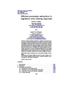
the AIC criterion is known to frequently select an "overparametrized" model resulting in a large mean square error as explained above when discussing possible effects of overfitting the simulated models. Even though the main goal of the present simulation study is to examine the overall performance of the estimators for typical stationary models with moderate AR and MA coefficients, it is of interest to see how the methods perform for nearly non-stationary or non-invertible models, and thus to examine the limits of their applicability. We considered the following models for achieving this objective. 1) Almost unit root AR(1) models of the form Yt = φYt_x+Zu with φ = .9, .95, .99, 2) almost unit root MA(1) models of the form Yt = Zt + ΘZt-ι with θ = .9, .95, .99. Our findings can be summarized as follows. Focusing first on AR models, the periodogram and semiparametric methods fail. The FAR BIC method by contrast gives estimates almost as good as for AR processes with moderate coefficients considered in Table 1. By contrast, for the almost unit root MA(1) models, the performance of the FAR BIC method is worse than that for the models considered in Table 1, and, also, as compared with the ARFIMA BIC method. A main reason why the performance of the ARFIMA(1, d, 1) method is noticeably better for this class of models than that of all other methods is that the ARFIMA(l,d, 1) model just includes the simulated ARFIMA(0,d, 1) and ARFIMA(l,d,O) models as its special case and yet avoids the parameter identification difficulties (Hannan (1970), p. 388) associated with fitting ARFIMA(p,d,g) models with p > l,g > 1. A detailed analysis of the simulation results for MA(1) models revealed that the ARFIMA(l,c/, 1) method yields estimates of the autoregressive and moving average coefficients which are within 0.1 of the correct values 0 and 0, respectively, and thus its estimate of d is based on an almost MA(1) short memory component. To illustrate the relative behaviour of the estimators in the infinite variance setting, we simulated symmetric α-stable innovations Zt with a = 1.5 and unit scale parameter. The nominal value of d is .2, which lies approximately in the middle of the stationary invertible range 0 < d < 1 — I/a specified in Assumption 3. Figures 1-4 show histograms of the estimated values of d in 50 replications of models I, II, V and VI. Only six methods were considered, namely, Periodogram, ARFIMA(l,d, 1), FAR AIC, FAR BIC, ARFIMA AIC and ARFIMA BIC. For all four models, the periodogram method provides a biased as well as a highly dispersed estimate of d, a finding that accords with the results reported above in Tables 1 and 2 for the the Gaussian case. Somewhat surprisingly, however, a similar comment applies to the ARFIMA BIC method, which, unlike the Gaussian case, now provides a biased estimator for all four models, and for models V and VI the estimator is also highly dispersed. A


143

Figure 1: FIGURE 1. Histograms of the estimated values of d for model I (ARFIMA(0,d,0)) with d = 0.2 and stable innovations. Periodogram

FARIMA(1,d,1)

I

FAR AIC

I 0.0

0.1

0.2

0.3

0.2

0.3

0.4

0.5

0.0

0.1

FARIMA AIC

FAR BIC

0.0

0.1

0.4

0.5

0.2

0.3

0.4

0.5

O.4

0.5

FARIMA BIC

0.4

0.5

0.0

0.1

0.2

I 0.3

plausible explanation for this behaviour is not easily given, but the simulations appear to indicate that the question of model selection for an α-stable ARFIMA process requires further investigation and that a naive use of the BIC criterion (5.4) may not be recommended in a situation where "outliers" may be present. The simulation results for the FAR BIC method, by contrast, broadly support the asymptotic consistency property established in Theorem 4.1. For models I and VI, in particular, the histogram is centred around the actual generated value of d = 0.2 with a relatively small dispersion around this value. For model V, however, the estimate is biased, probably reflecting the difficulty of estimating d for processes with a short memory MA component. In conclusion, the simulations indicate that when the long-memory process generating the observed series can be well approximated by a fractional autoregressive process, the method proposed in this paper provides a good estimator of d even when the order of the generating process, finite or infinite, is unknown, and in this sense it is "non-parametric". The method, moreover, compares favourably with the periodogram based non-parametric methods, which in this situation tend to have a larger variance and often a greater bias.


144

Figure 2: FIGURE 2. Histograms of the estimated values of d for model II (ARFIMA(l,d,O)) with d - 0.2 and stable innovations. Periodogram

0.0

0.1

0.2

0.3

0.4

0.5

FAR BIC

0.2

6

0.3

FAR AIC

FARIMA(1,d,1)

_ι I. 0.0

0.1

0.2

0.3

0.4

0.5

0.0

J I. 0.1

0.4

0.5

L.

0.2

0.3

0.4

0.5

0.4

0.5

FARIMA BIC

FARIMA AIC

0.0

0.1

0.2

0.3

Data Example

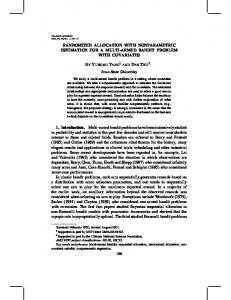
We consider the Ethernet traffic data studied by Leland et al (1994), Willinger et al (1995), Taqqu and Teverovsky (1997), among others. The data, described in detail by Leland et al (1994), were collected between August 1989 and February 1992 at the Bellcore Morristown Research and Engineering Center and represent the number of bytes per 10 milliseconds passing through a monitoring system during a "normal traffic hour" in August 1989. The periodogram of the data has a number of very sharp peaks at non-zero frequencies suggesting that the data may not necessarily follow an ARFIMA model. Taqqu and Teverovsky (1997) used a graphical analysis of the periodogram and the semi-parametric method to infer that the true value of d lies between 0.31 and 0.35. We consider here 18 consecutive 200 second long time periods making up the "normal traffic hour". Thus, we consider 18 extremely long series, each consisting of 20,000 observations. Because of the self-similarity property, the long memory parameter for each of the 18 time series must be the same, and the estimates should lie in the range between .31 and .35. Figure 5. shows the estimates obtained using the FAR BIC, ARFIMA BIC, and Semiparametric


145

Figure 3: FIGURE 3. Histograms of the estimated values of d for model V (ARFIMA(O,d,l)) with d = 0.2 and stable innovations. Periodogram

0.0

0.1

0.2

O.3

FARIMA(1,d.1)

O.4

0.5

.Hi..

0.0

0.1

FAR BIC

0.0

0.1

0.2

0.3

FAR AIC

0.2

0.3

0.0

0.1

FARIMA AIC

0.4

0.5

0.0

-

0.1

0.2

0.3

0.2

0.3

0.4

0.5

0.4

0.5

FARIMA BIC

0.4

0.5

0.0

0.1

0.2

0.3

methods. Following the analysis of Taqqu and Teverovsky (1997), we used for the semiparametric method the lowest 1/128 of all frequencies to get clear of the peaks at non-zero frequencies. The estimates obtained using the FAR BIC and ARFIMA BIC methods appear to be more stable over time than those obtained using the semiparametric method. It is possible that the intensity of long range dependence decreased in the 7th period and increased in the 8th period, but the semiparametric estimates probably overestimate the magnitude of the change. Acknowledgements. The software used in Section 5 for the periodogram and semiparametric methods and for simulating α-stable ARFIMA series was kindly made available to us by Murad Taqqu and Vadim Teverovsky, who also gave us plentiful advice on how to use it. Our colleague Simon Fear has invariably been willing to help us deal with intricacies of WΓ^X. and S+. We also thank Jan Beran for a discussion which stimulated the present research and Murad Taqqu for providing us with the Ethernet data studied in Section 6. Clifford Hurvich, Carenne Ludeήa, Adrian Raftery and Gennady Samorodnitsky also offered valuable comments.


146

Figure 4: FIGURE 4. Histograms of the estimated values of d for model VI (ARFIMA(l,d,l)) with d = 0.2 and stable innovations. FARIMA(1,d,1)

Periodogram

0.0

0.1

0.2

0.3

0.4

0.0

0.5

0.1

0.0

0.1

0.2

0.2

0.3

0.4

0.2

0.5

0.3

0.4

0.3

0.4

0.5

0.4

O.S

FARIMA BIC

FARIMA AIC

FAR BIC

0.5

0.0

0.1

0.2

0.3

Figure 5: FIGURE 5. Estimated long memory parameter for 18 consecutive Ethernet data series by various methods. FAR BIC: continuous, ARFIMA BIC: dotted, Semiparametric: dashed.

Y

,- \ ••

:

Λ. *

\\ / /

^

5

'

\

//••»'

"ΪJi ψj 1O

V •••. \

\

OS

\ "\ V

V

\

15

Series Number

References Agiakloglou, C, Newbold, P. and Wohar, M. (1993). Bias in an estimator of the


147

fractional difference parameter. Journal of Time Series Analisis, 14, 235-246. Akaike, H. (1978). A Bayesian analysis of the minimum AIC procedure. Ann. Inst. Statist. Math., 30 A, 9-14. Andel, J. (1986). Long memory time series models. Kybernetika, 22, 105-123. Bardet, J-M., Moulines, E. and Soulier, P. (1999). Recent advances on the semiparametric estimation of the long-range dependence coefficient. In ESAIM Proceedings, pp. 23-43. Societe de Mathematiques Appliquees et Industrielles. Beran, J. (1992). Statistical methods for data with long-range dependence. Statistical Science, 7, number 4, 404-416; With discussions and rejoinder, pages 404-427. Beran, J. (1994). Statistics for long-memory processes. Chapman & Hall, New York. Beran, J. (1995). Maximum likelihood estimation of the differencing parameter for invertible short and long memory autoregressive integrated moving average models. J. Royal Statist. Soc. B, 57, 659-673. Beran, J. (1997). Discussion of 'Heavy tail modelling and teletraffic data'. The Annals of Statistics, 25, 1852-1856. Beran, J., Bhansali, R. J. and Ocker, D. (1998). On unified model selection for stationary and nonstationary short- and long-memory autoregressive processes. Biometrika, 85, 921-934. Berk, K. N. (1974). Consistent autoregressive spectral estimates. The Annals of Statistics, 2, 489-502. Bhansali, R. J. (1978). Linear prediction by autoregressive model fitting in the time domain. The Annals of Statistics, 6, 224-231. Bhansali, R. J. (1980). Autoregressive and window estimates of the inverse correlation function. Biometrika, 67, 551-566. Bloomfield, P. (1973). An exponential model for the spectrum of a scalar time series. Biometrika, 60, 217-226. Box, G. E. P. and Jenkins, G. M. (1970). Time series analysis; forecasting and control. Holden Day, New York. Brockwell, P. J. and Davis, R. A. (1991). Time Series: Theory and Methods. Springer-Verlag, New York. Chan, N. H. and Palma, W. (1998). State space modeling of long-memory processes. The Annals of Statistics, 26, 719-740. Crato, N. and Ray, B. K. (1996). ModeΓselection and forecasting of long-range dependent processes: results of a simulation study. Journal of Forecasting, 15, 107-125. Dahlhaus, R. (1989). Efficient parameter estimation for self similar processes. Ann. Stat, 17, number 4, 1749-1766.

148


Fox, R. and Taqqu, M. S. (1986). Large-sample properties of parameter estimates for strongly dependent stationary Gaussian time series. The Annals of Statistics, 14, 517-532. Geweke, J. and Porter-Hudak, S. (1983). The estimation and application of long memory time series models. Journal of Time Series Analysis, 4, 221-238. Giraitis, L., Robinson, P. and Surgailis, D. (1999). Variance-type estimation of long memory. Stochastic Processes and their Applications, 80, 1-24. Giraitis, L. and Surgailis, D. (1990). CLT for quadratic forms in strongly dependent linear variables and application to asymptotical normality of Whittle's estimate. Prob. Th. Rel Fields, 86, 87-104. Granger, C. W. J. and Joyeux, R. (1980). An introduction to long-memory time series and fractional differencing. J. Time Series Anal, 1, 15-30. Hall, P. (1997). Defining and measuring long-range dependence. Fields Institute Communications, 11, 153-160. Hannan, E. J. (1970). Multiple Time Series. Wiley, New York. Hannan, E. J. (1973). The asymptotic theory of linear time series models. J. Appl. Prob., 10, 130-145. Hannan, E. J. (1980). The estimation of the order of an ARMA process. The Annals of Statistics, 8, 1071-1081. Hannan, E. J. and Quinn, B. G. (1979). The determination of the order of an autoregression. J. Royal Statist. Soc. B, 41, 190-195. Haslett, J. and Raftery, A. E. (1989). Space-time modelling with long-memory dependence: assesing Ireland's wind power resource. Appl. Statist, 38, number 1, 1-50. Heyde, C. C. and Yang, Y. (1997). On defining long-range dependence. J. Appl. Probab., 34, 939-944. Hosking, J. R. M. (1981). Fractional differencing. Biometrika, 68, number 1, 165-176. Hosking, J. R. M. (1984). Modeling persistence in hydrological time series using fractional differencing. Water Resources Research, 20, number 12, 1898-1908. Hurvich, C. M. and Beltrao, K. I. (1993). Asymptotics for the low-frequency ordinates of the periodogram of a long-memory time series. Journal of Time Series Analysis, 14, 455-472. Hurvich, C. M. and Brodsky, J. (2001). Broadband semiparametric estimation of the memory parameter of a long-memory time series using fractional exponential models. Journal of Time Series Analysis, 22, 221-249. Hurvich, C. M., Deo, R. and Brodsky, J. (1998). The mean squared error of Geweke and Porter-Hudak's estimator of the memory parameter of a long memory time series. Journal of Time Series Analysis, 19, 19-46.


149

Kokoszka, P. S. (1996). Prediction of infinite variance fractional ARIMA. Probability and Mathematical Statistics, 16/1, 65-83. Kokoszka, P. S. and Taqqu, M. S. (1995). Fractional ARIMA with stable innovations. Stochastic Processes and their Applications, 60, 19-47. Kokoszka, P. S. and Taqqu, M. S. (1996a). Infinite variance stable moving averages with long memory. Journal of Econometrics, 73, 79-99. Kokoszka, P. S. and Taqqu, M. S. (1996b). Parameter estimation for infinite variance fractional ARIMA. The Annals of Statistics, 24, 1880-1913. Kokoszka, P. S. and Taqqu, M. S. (1999). Discrete time parametric models with long memory and infinite variance. Mathematical and Computer Modelling, 29, 203-215. Kύnsch, H. (1987). Statistical aspects of self-similar processes. Bernoulli, 1, 67-74. Leland, W. E., Taqqu, M. S., Willinger, W. and Wilson, D.V. (1994). On the selfsimilar nature of Ethernet traffic (extended version). IEEE/ACM Transactions on Networking, 2, 1-15. Mikosch, T., Gadrich, T., Klύppelberg, C. and Adler, R. J. (1995). Parameter estimation for ARM A models with infinite variance innovations. The Annals of Statistics, 23, 305-326. Moulines, E. and Soulier, P. (1999). Broad band log-periodogram regression of time series with long range dependence. The Annals of Statistics, 27, 1415-1439. Pai, J. S. and Ravishanker, N. (1996). Bayesian modelling of arfima processes by markov chain monte-carlo methods. Journal of Forecasting, 15, 63-82. Pai, J. S. and Ravishanker, N. (1998). Bayesian analysis of autoregressive fractionally integrated moving average. Journal of Time Series Analysis, 19, 99-102. Parzen, E. (1969). Multiple time series modelling. In Multivariate Analysis II, New York (ed. P. R. Krishnaiah). Academic Press. Priestley, M. B. (1981). Spectral Analysis and Time Series: Volume 1. Academic Press. Ravishanker, N. and Ray, B. K. (1997). Bayesian analysis of vector arfima processes. Austral J. Statist, 39, 295-311. Robinson, P. M. (1995a). Log-periodogram regression of time series with long range dependence. The Annals of Statistics, 23, 1048-1072. Robinson, P. M. (1995b). Gaussian semiparametric estimation of long range dependence. The Annals of Statistics, 23, 1630-1661. Samorodnitsky, G. and Taqqu, M. S. (1994). Stable Non-Gaussian Random Processes: Stochastic Models with Infinite Variance. Chapman & Hall. Schwarz, G. (1978). Estimating the dimension of the model. The Annals of Statistics, 6, 461-464. Shibata, R. (1980). Asymptotically efficient selection of the order of the model for estimating parameters of a linear process. The Annals of Statistics, 8, 147-164.

150


Shibata, R. (1981). An optimal autoregressive spectral estimate. The Annals of Statistics, 9, 300-306. Sowell, F. B. (1992). Maximum likelihood estimation of stationary univariate fractionally integrated time series models. Journal of Econometrics, 53, 165188. Taqqu, M. S. and Teverovsky, V. (1997). Robustness of Whittle-type estimates for time series with long-range dependence. Stochastic Models, 13, 723-757. Taqqu, M. S. and Teverovsky, V. (1998). On estimating the intensity of long-range dependence in finite and infinite variance series. In A practical guide to heavy tails: Statistical techniques for analyzing heavy tailed distributions, Boston (eds R. Adler, R. Feldman and M. S. Taqqu), pp. 177-217. Birkhauser. Willinger, W., Taqqu, M. S., Leland, W. E. and Wilson, D.V. (1995). Self-similarity in high-speed packet traffic: analysis and modeling of Ethernet traffic measurements. Statistical Science, 10, 67-85.