Jul 24, 2008 - arXiv:0807.3916v1 [math.GN] 24 Jul 2008 ...... Further, the join of a subset Z â S is an element V Z of S which is the least upper bound of the ...
arXiv:0807.3916v1 [math.GN] 24 Jul 2008
´ Etale groupoids as germ groupoids and their base extensions∗ Dmitry Matsnev and Pedro Resende
Abstract We introduce the notion of wide representation of an inverse semigroup and prove that with a suitably defined topology there is a space of germs of such a representation which has the structure of an ´etale groupoid. This gives an elegant description of Paterson’s universal groupoid and of the translation groupoid of Skandalis, Tu, and Yu. In addition we characterize the inverse semigroups that arise from groupoids, leading to a precise bijection between the class of ´etale groupoids and the class of complete and infinitely distributive inverse monoids equipped with suitable representations, and we explain the sense in which quantales and localic groupoids carry a generalization of this correspondence. Keywords: coarse geometry, complete inverse semigroup, germ groupoid, localic groupoid, quantale, topological ´etale groupoid, translation groupoid, universal groupoid. 2000 Mathematics Subject Classification: 20M18, 22A22, 54H10
1
Introduction
The local bisections of a topological ´etale groupoid G can be identified with the open subsets of the space of arrows on which the domain and the range maps are injective. The set of all the local bisections of G forms an inverse semigroup, denoted by I(G). This inverse semigroup is equipped with a natural representation on the space G0 of units of G, that is a homomorphism to the inverse semigroup of partial homeomorphisms on the space of units. This Research supported in part by Funda¸ca˜o para a Ciˆencia e a Tecnologia through FEDER and project PPCDT/MAT/55958/2004. ∗
1
representation is full in the sense that the idempotents of I(G) bijectively correspond to the open sets of G0 . On the other hand, for any inverse semigroup S equipped with a full representation on a topological space X, its space of germs with a sheaf-like topology can be given a structure of ´etale groupoid with X as unit space. The first objective of this paper is to extend the aforementioned germ groupoid construction to the following more general case, where an inverse semigroup S represented on a topological space X will be called wide over X if the images of the idempotents in S under the representation cover X: Theorem. For any wide inverse semigroup over a topological space X, its space of germs can be given the structure of an ´etale groupoid with object space X. An immediate application of this theorem is the following extension procedure for ´etale groupoids: (1) start with an ´etale groupoid G plus the full representation of I(G) on G0 ; (2) define an extension X of the space G0 in such a way that I(G) becomes a wide inverse semigroup over X; (3) apply the above theorem in order to obtain an ´etale groupoid which is the required “base extension” of the original one. The second objective of this paper is to describe how two classical constructions in the theory of ´etale groupoids can be achieved using the germ groupoid approach. The first example is the universal groupoid of Paterson, a certain ´etale groupoid associated to a countable inverse semigroup, with the properties that the C ∗ -algebras for the semigroup and its groupoid are the same, both the full and the reduced ones. The original construction [5] relies on so-called localisation techniques due to [3]; we show that it can be described more succinctly in terms of the above theorem, as the germ groupoid associated to a wide representation. Concerning the second example, suppose we start with a discrete groupoid G (this is the same as an ´etale groupoid whose unit space is discrete). Then the representation of the underlying inverse semigroup can be extended to a ˇ representation by partial homeomorphisms on the Stone–Cech compactification of the unit space of G. Taking the germs of this extension, we obtain an ´etale groupoid β0 G, which extends G in such a way that its unit space ˇ is the Stone–Cech compactification of the unit space of G. The arrows of β0 G are simply the arrows of G and the other necessary ones required by the structure laws (hence β0 G can be viewed as the most economical extension of G with the required space of units). This result is closely related to work of Skandalis, Tu, and Yu, who in [8] established the connection between ´etale groupoids and coarse metric spaces 2
(see [9]). They defined the translation groupoid of a boundedly discrete coarse space as the maximal possible principal ´etale extension of the pair groupoid on that space such that the unit space of the extension is the ˇ Stone–Cech compactification of the space we started with. The coarse Baum– Connes conjecture for the original space is then equivalent to the Baum– Connes conjecture for its translation groupoid. As a consequence of that, for example, the Hilbert space embeddability for a discrete space implies the coarse Baum–Connes conjecture for such a space, and, via the Higson descent technique, one gets an elegant proof of the Novikov conjecture for discrete groups equipped with the Hilbert space embeddings. If we take the inverse semigroup generated by controlled partial bijections of X (see [9]) with its tautological representation on X and extend it via the ˇ Stone–Cech technique described above, the resulting inverse semigroup represented on βX is often wide, for instance when the coarse space X is unital (e.g., this happens when the coarse structure comes from the equivalence class of metrics, which is particularly relevant for the Novikov conjecture). In such a case the translation groupoid can be obtained by our germ groupoid construction. Finally, as a third objective we obtain a precise characterization of the inverse semigroups of the form I(G) and a bijection (up to isomorphisms) between the class of ´etale groupoids with unit space X and the class of complete inverse semigroups equipped with full representations on X. The particular case where X is a sober space leads, via [7], to a connection with localic groupoids (internal groupoids in the category of locales) and quantales, whose significance in the context of the present paper we also describe. The paper is structured as follows. In Section 2 we recall the notions of inverse semigroup, inverse semigroup representation, ´etale groupoid, and germs. We continue with the structure theorems connecting these notions and then introduce wide representations. The main result of this section is the theorem stated above. Section 3 is devoted to the discussion of the ˇ universal groupoid of Paterson. In Section 4 we present the Stone–Cech extension technique for discrete groupoids. We review the translation groupoid of Skandalis, Tu, and Yu, and discuss how it arises as a germ groupoid. Finally, in Section 5 we close the circle by characterizing the inverse semigroups that arise from ´etale groupoids (as described in Section 2). This requires us to address the order-theoretic properties of inverse semigroups and, in particular, the notion of complete inverse semigroup. We conclude with the remarks on localic groupoids and quantales that establish the relation to [7].
3
2
Germ groupoids of inverse semigroups
Inverse semigroups Definition 2.1 Let S be a semigroup. An element t ∈ S is said to be an inverse of s ∈ S if sts = s and tst = t. An inverse semigroup S is a semigroup such that for all s ∈ S there is a unique inverse of s, which we shall denote by s∗ . Equivalently, an inverse semigroup is a semigroup for which each element has an inverse and for which any two idempotents commute (see [4]). The set of idempotents is denoted by E(S). An inverse monoid is an inverse semigroup that has a multiplicative unit, which we shall denote by e. A few simple but useful facts about inverse semigroups are: 1. In any inverse semigroup the inverse operation defines an involution. 2. The set of idempotents forms a semilattice with meet given by multiplication: f ∧ g = f g; this semilattice has a greatest element if and only if S is a monoid. 3. The idempotents are precisely the elements of the form ss∗ . 4. A semigroup homomorphism between inverse semigroups automatically preserves inverses. Let X be a topological space, and let I(X) be the set of all the partial homeomorphisms on X, by which we mean the homeomorphisms h : U → V with U and V open sets of X. This set has the structure of an inverse semigroup; its multiplication is given by composition of partial homeomorphisms wherever this composition is defined: if h : U → V and h′ : U ′ → V ′ are partial homeomorphisms then their product is the partial homeomorphism hh′ : h−1 (V ∩ U ′ ) → h′ (V ∩ U ′ ) defined at each point of its domain by (hh′ )(x) = h′ (h(x)), and the semigroup inversion is the usual inverse of a homeomorphism: h:U →V
7→
h∗ = h−1 : V → U .
Definition 2.2 Let X be a topological space. By a pseudogroup over X will be meant any subset P ⊂ I(X) which is closed under the multiplication 4
and the inverse of I(X). A pseudogroup P over X is full if it is also closed under identities in the sense that idU ∈ P for every open set U ⊂ X; and it is complete if it is full and for all h ∈ I(X) and every open cover (Uα ) of dom(h) we have h ∈ P if h|Uα ∈ P for all α. The Wagner–Preston theorem (see [4]) asserts that every inverse semigroup is isomorphic to a pseudogroup. However, we shall need more precise terminology: Definition 2.3 Let S be an inverse semigroup. By a representation of S on a topological space X will be meant a semigroup homomorphism ρ : S → I(X). The representation is full if ρ restricts to an isomorphism E(S) → E(I(X)) ∼ = Ω(X). By an inverse semigroup over X will be meant a pair (S, ρ) consisting of an inverse semigroup S equipped with a representation ρ : S → I(X). If ρ is full (in this case S is necessarily a monoid) then (S, ρ) is said to be a full inverse semigroup over X. Finally, an inverse monoid representation is called unital if it preserves the unit.
´ Etale groupoids To start, let us briefly fix notation for groupoids. Definition 2.4 A (topological) groupoid G is a pair of topological spaces, the space of arrows G1 and the space of objects G0 , equipped with continuous maps i
G2
m
r u
� /
G1 o
/ /
G0 ,
d
where G2 is the set G1 ×G0 G1 of composable pairs of arrows, G2 = {(x, y) ∈ G1 × G1 | r(x) = d(y)} , equipped with the subspace topology relative to the product topology on G1 × G1 (i.e., the pullback of d and r in the category of topological spaces). The maps m, d, r, i, and u are the multiplication, domain, range, inverse, and unit maps, respectively. To shorten notation, we shall contract m(x, y) to xy, i(x) to x−1 , and u(x) to 1x . We require these maps to satisfy the usual groupoid axioms. We shall be mostly concerned with ´etale groupoids, in other words with those for which the domain map d is a local homeomorphism, or, equivalently, for which d is open and u(G0 ) is open in G (see [7] for the latter characterization). 5
By a local bisection of an ´etale groupoid G is usually meant a local section s : U → G1 of the domain map d on an open set U ⊂ G0 such that r ◦ s is an open embedding of U into G0 . Often we shall, usually without any comment, identify the local bisections s with their images s(U), which are the open subsets V of G1 such that the restrictions d|V and r|V are both injective (these sets are called G-sets in [5], following terminology introduced in [6], but we shall avoid this because it clashes with the established terminology for sets equipped with an action of a group G). Definition 2.5 Let G be an ´etale groupoid. The inverse semigroup of G, I(G), is the set of local bisections of G, with multiplication given by pointwise multiplication of (images of) local bisections, and the inverse being similarly calculated pointwise. We remark that I(G) acts partially on G0 and in fact is a full inverse semigroup over G0 , with the representation ρG : I(G) → I(G0 ) defined by ∼ =
ρG (V ) : d(V ) → r(V ) ρG (V )(d(x)) = r(x) for each V ∈ I(G) and x ∈ V . Definition 2.6 Let (S, ρ) be a full inverse semigroup over a topological space X. We define the germ of s ∈ S at x ∈ dom(ρ(s)) to be germx s = {t ∈ S|∃f ∈ E(S) : f t = f s, x ∈ dom(ρ(t)) ∩ dom(ρ(f ))}, and the set of germs of (S, ρ) to be Germs(S, ρ) = {(x, germx s)|x ∈ X, s ∈ S}. We equip Germs(S, ρ) with the sheaf topology, whose basis consists of open sets of the form, for each s ∈ S, (2.7)
Us = {(x, germx s) | x ∈ dom(ρ(s))} .
These two constructions can be regarded as inverse to each other, with the connection given by the following theorems (in Section 5 we shall describe conditions on the inverse semigroups under which the two constructions are really inverse to each other): Theorem 2.8 Let (S, ρ) be a full inverse semigroup over a topological space X. Then the space Germs(S, ρ) can be given the structure of an ´etale groupoid with object space X. 6
Proof. This construction is an essentially straightforward adaptation of the construction of a local homeomorphism of a sheaf and is done in [5] in a slightly more general setting, namely when ρ(E(S)) is only a basis of X rather than the whole topology. Although also subject to restrictions pertaining to the space X, which in [5] has to be Hausdorff, second countable, and locally compact, these restrictions are irrelevant, so we shall describe the construction for full inverse semigroups here. The groupoid G = Germs(S, ρ) has the set of arrows G1 = {(x, germx s)| s ∈ S and x ∈ dom(ρ(s))} .1 Note that the projection d : Germs(S, ρ) → X defined by (x, germx s) 7→ x is a local homeomorphism. Also, the subspace topology on X ⊂ Germs(S, ρ) coincides with the original topology on X. Keeping all these things in mind, we can introduce the topological groupoid structure on the space of germs. Namely, the operations are defined as follows: d(x, germx s) r(x, germx s) 1x (x, germx s)(ρ(s)(x), germρ(s)(x) , t)
= = = =
x ρ(s)(x) (x, germx e) (x, germx (st))
(x, germx s)−1 = (ρ(s)(x), germρ(s)(x) (s∗ )) . This groupoid is ´etale, for the domain map d is a local homeomorphism as mentioned above. We do not give a direct proof of the soundness of this construction here, since it is similar to that of [5]. Now we prove that every ´etale groupoid arises in this way: Theorem 2.9 Let G be an ´etale groupoid, and let ρG : I(G) → I(G0 ) be its full representation. Then Germs(I(G), ρG ) ∼ = G. Proof. The standard identification of the total space E of a local homeomorphism p : E → X with the space of stalks (germs of continuous local sections) of the sheaf of local sections of p gives us a homeomorphism between Germs(I(G), ρG ) and G, since it is clear that every local section is locally a local bisection: if x ∈ U and s : U → G1 is a local section of d then there is an open set V ⊂ U such that x ∈ V and s|V is a local bisection. It is then routine to check that the groupoid operations in Germs(I(G), ρG ) correspond to those in G. 1
The arrows are pairs (x, germx s) rather than just the actual germs germx s because unless X is a T0 -space we may have germx s = germy s with x 6= y — see also Section 5.
7
Unital representations of inverse monoids We have seen that any ´etale groupoid G is determined by a full representation of I(G) on the unit space G0 , but we shall need to extend this relationship to encompass more general inverse semigroup representations, in particular, in this section we shall see explicitly how any unital representation of an inverse monoid can be turned into a full representation of a larger inverse monoid. Let M be an inverse monoid, X a topological space, and ρ : M → I(X) a monoid homomorphism, that is, a unital representation in our terminology. Define (Ω(X) ↓ M) = {(U, s) | U ∈ Ω(X), s ∈ M, U ⊂ dom(ρ(s))} , where the pair (U, s) should be thought of as a formal restriction of s to the subspace U of its domain. Lemma 2.10 The set (Ω(X) ↓ M) has a structure of inverse monoid. Proof. The multiplication can be defined by (U, s)(V, t) = (U ∩ ρ(s)−1 (V ∩ ρ(s)(U)), st) , the inverse by (U, s)∗ = (ρ(s)(U), s∗ ) , and the unit is (X, e). The rest is straightforward. The monoid (Ω(X) ↓ M) is too large for the purposes we have in mind because we shall need the submonoid of idempotents to be isomorphic to Ω(X), whereas in E(Ω(X) ↓ M) there are in general many copies of each open set, namely (U, f ) for each idempotent f of M such that U ⊂ dom(ρ(f )). Hence, we shall define a quotient of (Ω(X) ↓ M) in order to get a full inverse monoid over X. To do this, define an equivalence relation on (Ω(X) ↓ M) by (U, s) ∼ (V, t) if U = V and there is f ∈ E(M) such that U ⊂ dom ρ(f ) and f s = f t. It is easy to see that this is indeed a congruence relation. We shall denote the congruence class of (U, s) by [U, s] and the quotient (Ω(X) ↓ S)/∼ by MX . Lemma 2.11 MX is an inverse monoid and it is equipped with a full representation ρX : MX → I(X) given by (2.12)
ρX ([U, s]) = ρ(s) |U ,
s ∈ M, 8
U ⊂ dom(ρ(s)) .
Proof. If (U, s) ∼ (U, s′ ) and (V, t) ∼ (V, t′ ) then we have f, g ∈ E(M) with f s = f s′ and gt = gt′ , and U and V are inside dom(ρ(f )) and dom(ρ(g)) respectively. We first claim that the compositions (U, s)(V, t) and (U, s′ )(V, t) represent the same class in MX . Indeed, ρ(f s) = ρ(f s′ ) implies ρ(s) |U = ρ(s′ ) |U , so that U ∩ ρ(s)−1 (V ∩ ρ(s)(U)) = U ∩ ρ(s′ )−1 (V ∩ ρ(s′ )(U)), which means that the “domain” of the composition is well defined. Next, f st = f s′ t and clearly f is an idempotent for which the domain U ∩ ρ(s)−1 (V ∩ ρ(s)(U)) of the compositions under consideration lies inside U, which, in turn, is inside dom(ρ(f )) by assumption. By a similar computation, now involving g and the appropriate domains, we obtain (U, s′)(V, t) ∼ (U, s′ )(V, t′ ) and, together with our previous observation, this leads to (U, s)(V, t) ∼ (U, s′ )(V, t′ ) as desired. For inverses, take (U, s) ∼ (U, s′ ) with f ∈ E(M) as above. A trivial computation reveals that (s′∗ f s′ )(s∗ f s)s∗ = (s′∗ f s′ )(s∗ f s)s′∗ , so that (U, s)∗ ∼ (U, s′ )∗ using an idempotent s′∗ f s′ s∗ f s whose “domain” clearly contains ρ(s)(U). The congruence class [X, e] provides the unit, and so we indeed have an inverse monoid. Now we prove that the map ρX of (2.12) is a representation. It is well defined because ρX [U, s] gives us a partial homeomorphism of X by definition. Moreover, it preserves multiplication, inverses and the unit. Say, ρX ([U, s][V, t]) = ρX [ρ(s)−1 (V ∩ ρ(s)(U)), st] = ρ(st)|ρ(s)−1 (V ∩ρ(s)(U )) , while ρX [U, s]ρX [V, t] = ρ(s)|U ρ(t)|V , and these two partial homeomorphisms of X are the same in I(X). Further, the representation ρX is full, since for every U ∈ Ω(X) the class [U, e] gives an idempotent in MX whose image is idU . Note that we have the following commuting square of inverse monoid homomorphisms with the vertical homomorphism Ω(X) → MX mapping an 9
open set U to [U, e] and the horizontal homomorphism M → MX mapping s to [dom(ρ(s)), s]: E(M)
dom ρ
/
Ω(X)
⊂
� � /
M
MX
We remark that MX in general is not a pushout in the category of inverse monoids. However, it has the following universal property. Lemma 2.13 Let M ′ be an inverse monoid for which there exist inverse monoid homomorphisms α and β making the outer square of the following diagram E(M)
dom ρ
/
Ω(X)
⊂
(2.14)
�
M
� /
β
MX ρ′ α
,
# �
M′
commutative. Suppose also that β(U ∩ ρ(s−1 )(V ∩ ρ(s)(U)))α(s) = β(U)α(s)β(V ) and α(s∗ )β(U) = β(ρ(s)(U))α(s∗ ) for all U, V ∈ Ω(X) and s ∈ M with U ⊂ dom(ρ(s)). Then there exists a unique inverse monoid homomorphism ρ′ : MX → M ′ as depicted in (2.14). Proof. First note that in M we have a decomposition (U, s) = (U, e)(dom(ρ(s)), s),
U ∈ Ω(X), s ∈ M, U ⊂ dom(ρ(s)),
which in turn provides us with a similar decomposition for MX : [U, s] = [U, e][dom(ρ(s)), s]. Thanks to this decomposition, ρX [U, s], if it exists, has to be ρ′ [U, e]ρ′ [dom(ρ(s)), s] ,
10
but both of the terms [U, e] and [dom(ρ(s)), s] come from the preimages U in Ω(X) and s in M respectively, so that we can define the results of applying ρ′ to them using β and α: ρ′ [U, s] = β(U)α(s),
U ∈ Ω(X), s ∈ M, U ⊂ dom(ρ(s)).
Thus we obtain uniqueness of ρ′ . To check existence, that is, to see that the formula above gives us a homomorphism, we check that ρ′ ([U, s][V, t]) = ρ′ ([U ∩ ρ(s−1 )(V ∩ ρ(s)(U)), st]) = β(U ∩ ρ(s−1 )(V ∩ ρ(s)(U))α(st) = β(U)α(s)β(V )α(t) = ρ′ ([U, s])ρ′ ([V, t]) and ρ′ ([U, s])∗ = (β(U)α(s))∗ = α(s∗ )β(U) = β(ρ(s)(U))α(s∗ ) = ρ′ ([ρ(s)(U), s∗ ]) = ρ′ ([U, s]∗ ). The commutativity of the resulting diagram comes automatically: starting with U ∈ Ω(X), it is being mapped to [U, e] in MX and then to β(U)α(e) in M ′ . But the latter product coincides with β(U), for α(e) is the unit of M ′ . For another side of the diagram, an element s in M is being first mapped to [dom(ρ(s)), s] in MX and after that via ρ′ to β(dom(ρ(s)))α(s). Consider an idempotent ss∗ whose “domain” clearly covers the one of s (in fact, they are the same) and trace it through the outer square in (2.14) to obtain β(dom(ρ(s))) = β(dom(ρ(ss∗ ))) = α(ss∗ ). Multiplying this identity by α(s) on the right, we get β(dom(ρ(s)))α(s) = α(s) as required. Of course, a pushout in the category of inverse monoids also exists, but any concrete description of such a pushout would require adding new idempotents sf s∗ for s ∈ M and f an “old” idempotent in M.
Germ groupoids revisited The germ groupoid of (MX , ρX ) from the previous section has a direct description in terms of the germ groupoid of (M, ρ), as we shall now see. Further, we exhibit this correspondence in an even more general context.
11
Definition 2.15 Let (M, ρ) be an inverse monoid over a topological space X (as usual, we assume that ρ is a unital representation). As in Definition 2.6, define the germ of s ∈ M at x ∈ dom(ρ(s)) to be germx s = {t ∈ M|∃f ∈ E(M) : f t = f s, x ∈ dom(ρ(t)) ∩ dom(ρ(f ))} and the space of germs to be Germs(M, ρ) = {(x, germx s)|x ∈ X, s ∈ M}. Further, we topologize the space of germs Germs(M, ρ) by making a topology basis out of the sets Vs,U = {(x, germx s)|x ∈ U} for s ∈ M and U ⊂ dom(ρ(s)), U ∈ Ω(X). Note that this sheaf topology is different from the one introduced in Theorem 2.8 before. We have a straightforward counterpart of Theorem 2.8: Theorem 2.16 Let (M, ρ) be a unital inverse monoid representation over a topological space X. Then the space Germs(M, ρ) can be given the structure of an ´etale groupoid with object space X. We shall not give a detailed proof of this theorem here, but mention that one defines all the structure maps exactly as in Theorem 2.8 before and thus obtains a groupoid with object space X. The only nontrivial part is to show that this groupoid is ´etale. We shall see that the groupoid in question is the same as the one for a full representation ρX obtained from ρ and thus reduce it to the case already discussed. Theorem 2.17 Let (M, ρ) be a unital inverse monoid representation over a topological space X and (MX , ρX ) — an induced full inverse monoid as constructed in the previous section. Then Germs(M, ρ) ∼ = Germs(MX , ρX ). Proof. We start by writing explicitly what germs in Germs(MX , ρX ) are. Take [U, s] ∈ MX and x ∈ dom(ρX ([U, s]) = dom(ρ(s)|U ) = U. Then (2.15) germx [U, s] = {[V, t] ∈ MX | ∃[F, f ] ∈ E(MX ) with x ∈ F, [F ∩ U, f s] = [F ∩ V, f t]} . 12
In order to identify this germ with germx s ∈ Germs(M, ρ), we check that t from [V, t] above also belongs to germx s. This is true, for clearly x ∈ V ⊂ dom(ρ(t)) and gf s = gf t for some g ∈ E(M) covering F ∩ U ∋ x. This shows that the mapping Germs(MX , ρX ) → Germs(M, ρ) :
germx [U, s] 7→ germx s
is surjective and well defined. To check the injectivity of such a correspondence, take germx [U, s] and germx [V, s] which are both mapped to germx s. In fact, for an idempotent [U ∩ V, e] of MX , its domain under ρX contains x and one has [U ∩ V, e][U, s] = [U ∩ V, e][V, s], which means that the germs are indeed the same, according to (2.15). Next, we clarify why the groupoid structure maps in Germs(M, ρ) and Germs(MX , ρX ) are the same. This is so because in the correspondence between germs established above the domains are x and the ranges are ρ(s)(x) = ρX ([U, s])(x). The inverses are germρ(s)(x) s∗ and germρX ([U,s])(x) [ρ(s)U, s∗ ] which clearly correspond to each other, the units 1x are defined using the germs of e and [X, e] respectively, which also correspond to each other. Finally, the composition is preserved as well: for two composable arrows germx [U, s] and germρ(s)(x) [V, t] in Germs(MX , ρX ) their composition is germx [U ∩ ρ(s)−1 (V ∩ ρ(s)(U)), st], which corresponds to germx (st) in Germs(M, ρ) as expected. We finish by checking that the topologies imposed on Germs(M, ρ) and Germs(MX , ρX ) are compatible. An elementary open set in the latter space, V[U,s] = {germx [U, s] | x ∈ dom(ρX ([U, s])) = U }, corresponds to Vs,U in the former one, and vice-versa, which completes the proof.
Wide representations of inverse semigroups Finally, we want to treat the following slightly more general case. Definition 2.18 A representation ρ : S → I(X) of an inverse semigroup S on a topological space X will be called wide if ρ(E(S)) covers E(I(X)). We shall refer to such S as a wide inverse semigroup over X.
13
In particular, any full representation is wide. More generally, any inverse monoid representation is a wide representation. For a rather extreme example, the Wagner–Preston representation of any inverse semigroup is wide. Given a wide inverse semigroup (S, ρ) over a topological space X, define the germ of s ∈ S at x ∈ dom(ρ(s)) and the space of germs exactly as above to be germx s = {t ∈ S|∃f ∈ E(S) : f t = f s, x ∈ dom(ρ(t)) ∩ dom(ρ(f ))} and Germs(S, ρ) = {(x, germx s)|x ∈ X, s ∈ S} respectively. The topology on the space of germs is generated by the basis consisting of Vs,U = {(x, germx s)|x ∈ U} for s ∈ S and U ⊂ dom(ρ(s)), U ∈ Ω(X), as for the unital monoid representation above. One can extend Theorem 2.16 to Theorem 2.19 For a wide inverse semigroup (S, ρ), the space Germs(S, ρ) can be given a structure of ´etale groupoid with object space X. Again, our goal is not to prove this theorem independently, but rather by means of connecting it with other constructions we have studied. Theorem 2.20 Let (S, ρ) be a wide inverse semigroup over a topological space X and the inverse monoid Se be the result of adjoining a unit to S. Further, extend ρ to a monoid representation ρe : ⊂
/ Se S CC CC CC ρe ρ CCC ! � I(X)
Then
Germs(S, ρ) ∼ = Germs(Se , ρe ).
Proof. Since we impose the same topology on the space of germs in both cases, all we need to check is that the spaces of germs are the same as sets. And this is indeed true, because ρ is wide and thus we just add the unit e to the germs that contain idempotents (this will “enrich” some germs, but it will not add any new ones). 14
Note that for Germs(Se , ρe ) all the units can be written as germs of e as in the full representation case which was not the case right away for wide representations. Corollary 2.21 Any wide inverse semigroup (S, ρ) over a topological space X determines an inverse monoid with a full representation on X, and their germ groupoids are isomorphic. We finish this section by mentioning that the notion of a wide inverse semigroup is more general than the localizations of [3, 5], since we do not impose any conditions on the topology of X and also do not require the idempotents to provide a basis for the topology, but just a cover.
3
Example: the universal groupoid of Paterson
We shall show that the universal groupoid of an inverse semigroup introduced in [5] can be obtained using our wide representation techniques. This section is intended to be as self-contained as possible, so we start by describing the construction and then comment on the properties of the universal groupoid and some motivations behind it. Let S a countable inverse semigroup. Consider the set X = {non-zero multiplicative functions x : E(S) → {0, 1}} . For each s in S let Ds denote the subset of X consisting of all the functions x for which x(ss∗ ) = 1. We topologize X by specifying as a basis for the topology the collection of all the sets Df ∩ (X\Df1 ) ∩ (X\Df2 ) ∩ · · · ∩ (X\Dfn ) where f, f1 , f2 , . . . , fn are idempotents of S such that f fi = fi for all i = 1, . . . n. In this way X becomes a locally compact totally disconnected space (and hence Hausdorff). Now we construct a representation ρu of S on X. For s ∈ S, we define a homeomorphism ρu (s) : Ds → Ds∗ by sending x ∈ Ds to y ∈ Ds∗ defined by y(f ) = x(sf s∗ ). It is easy to see that this representation is wide: for any x ∈ X there ought to be an idempotent f with x(f ) = 1, since x is not identically 0. 15
Then ρu (f ) is a partial identity of X with domain Df which tautologically contains x. Therefore we can construct the germ groupoid Gu corresponding to S and ρu as prescribed in the previous section. This groupoid is called the universal groupoid of S. It enjoys the following properties: 1. C ∗ (S) = C ∗ (Gu ). ∗ ∗ 2. Cred (S) = Cred (Gu ).
3. For any other ample S-groupoid G (see [5]), its unit space G0 is homeomorphic to a closed invariant subspace Y of (Gu )0 , and there exists a continuous open surjective S-equivariant homomorphism φ : Gu |Y → G, φ|Y = id. We comment that our construction, unlike the original one of Paterson in [5], does not appeal to the localisation techniques, and therefore does not require the inverse semigroup S to be countable (and the germ groupoid construction from the previous section does not require the space X to be locally compact Hausdorff in general). Of course, for the proof of the analytic properties of the universal groupoid listed above, these constrains are still required.
4
Example: the translation groupoid of Skandalis, Tu, and Yu
ˇ The Stone–Cech compactification via ultrafilters We start by briefly reviewing some elements of the construction of the Stone– ˇ Cech compactification of a discrete space, mostly to fix the notation. For more details the reader is referred to [2]. Definition 4.1 Let X be a space with the discrete topology. A collection F of subsets of X is called a filter if the following conditions are satisfied: • ∅∈ / F. • Whenever U ⊂ V for some subsets U, V of X, and U ∈ F , then V ∈ F . • For U, V ∈ F , U ∩ V ∈ F .
16
ˇ One can identify the Stone–Cech compactification of a discrete space X with the space of ultrafilters, which are by definition maximal (with respect to inclusion) filters of subsets of X. The topology on this space is generated by the sets ˜ = {F |U ∈ F }, U U ⊂ X. The embedding of X into βX for our discrete space case in this model is done by mapping x ∈ X to Fx , the principal filter at x which is defined to consist of all subsets of X which contain x. Further, if one identifies X with the image of its embedding into βX, any basic open set U˜ of βX has U as its trace on X. Moreover, given a set U in X, its closure in βX is precisely U˜ . We conclude this review with the following technical result. Lemma 4.2 Let U be a subset of a discrete space X. Then there exists a canonical homeomorphism between βU and U˜ (the latter one being a subset of the ambient space βX with the induced topology.) Proof. If we take some ultrafilter F in U˜ then the family FU := {F ∩ U|F ∈ F } is an ultrafilter in U. Conversely, given an ultrafilter G of subsets of U, one can formally define GX = {G ∪ A|G ∈ G, A ⊂ X\U}, which turns out to be an ultrafilter on X extending U. This correspon˜ is bijective (the dence between ultrafilters on U and the ones on X within U ‘shrinking’ and ‘enlarging’ procedures are inverse to each other). Under this correspondence the standard basis of the topology on βU, namely the one comprised out of the sets A˜ = {G ∈ βU|A ∈ G},
A ⊂ U,
corresponds (element-wise) to (4.3)
{F ∈ βX|A ∈ F }.
We claim that the latter sets are the intersections of the elements of the standard basis for βX with U˜ . Indeed, given V ⊂ X, U˜ ∩ V˜ = U^ ∩ V , so that taking A = U ∩ V the condition that V runs over all subsets of X is equivalent to that of A running over all subsets of U. This shows that the sets in (4.3) form a basis for U˜ in βX and, moreover, the correspondence which we established respects the aforementioned bases of the topologies, hence it is a homeomorphism. 17
ˇ The Stone–Cech compactification of the unit space Having a partial homeomorphism h : U → V between two subsets U, V of X, we can extend it to a homeomorphism βh : βU → βV or, equivalently, ˜ : U˜ → V˜ . by the virtue of Lemma 4.2, to a homeomorphism h ˇ Now we are in position to prove the Stone–Cech extension theorem for discrete groupoids. Theorem 4.4 Let G be a discrete groupoid. Then there exists an ´etale groupoid (which we shall denote by β0 G) such that G is a subgroupoid of β0 G and (β0 G)0 = βG0 . Proof. The inverse semigroup I(G) has a representation ρG on G0 (notice that all the partial homeomorphisms in this presentation are just partial bijections.) We extend it to ρf G : I(G) → I(βG0 ) by means of taking every partial homeomorphism h : U → V on G0 from ρG (I(G)) and extending it ˜ :U ˜ → V˜ on βG0 . It is easy to see that by to a partial homeomorphism h ] −1 ) ˜ −1 = (h doing such an extension we indeed obtain a representation: (h) ˜h ˜ ′ = hh f′ . and h Notice that whilst the representation ρG is full (so that ρG (E(I(G))) ∼ = ˜ Ω(G0 )), ρf is wide, due to the fact that ρ f (E(I(G))) contains all the sets U G G with U ∈ Ω(G0 ), which form a basis for Ω(βG0 ) and hence cover it. The statement now follows from a direct application of Corollary 2.21. To see that G is a subgroupoid of β0 G, recall that G can be identified with the germ groupoid Germs(I(G), ρG ). For any x ∈ G0 and any s ∈ I(G) with x ∈ dom(ρG (s)), the germ of s at x as an arrow in G can be viewed as an arrow in β0 G, since the representation ρf G coincides with ρG on X (more specifically, for x ∈ X, the conditions that x belongs to the domain of ρf G (t) and to the domain of ρ(t) for some t ∈ I(G), are equivalent. But aside from domain conditions, the definitions of the germs forming G and β0 G are the same.) Remark 4.5 In general (β0 G)1 6= βG1 , so that the newly constructed groupoid ˇ is not the Stone–Cech compactification of the original groupoid G.
Digression: the translation groupoid We shall discuss one more specialized case of the germ groupoid construction ˇ and the Stone–Cech extension when the inverse semigroup is a pseudogroup over a discrete topological space. The motivation for such a digression is that Skandalis, Tu, and Yu have proven that the coarse Baum–Connes conjectures 18
for the discrete coarse space and the resulting groupoid (which they called the translation groupoid ) are equivalent. Here we present a brief account of the ideas involved. For more details on the construction and the ambient context consult the original paper [8] of Skandalis, Tu, and Yu; a more comprehensive account on coarse geometry can be found in [9]. Let X be an infinite set endowed with the discrete topology. In what follows, it is convenient to regard X × X as a pair groupoid, that is, the groupoid with object space X, arrow space X × X, d and r being the first and second projections π1 , π2 : X × X → X, etc. Definition 4.6 A coarse structure on X is a collection E of nonempty subsets of X × X, called controlled sets, such that every singleton of X × X belongs to E and E is closed with respect to taking • Subsets; • Finite unions; • Inverses (forming a new set consisting of the inverses of the elements of the original set in the pair groupoid sense); • Products (forming a new set out of the products of all composable elements from two controlled sets); Such X together with a coarse structure is called a coarse space. One important example of coarse spaces comes from a metric. Starting from a metric space X, one can define the coarse structure to contain all sets E ⊂ X × X such that ∃N : ∀(x, y) ∈ E dist(x, y) < N. Not all coarse structures come from a suitable metric, however; in some important cases one can in principle impose different, yet equivalent metrics on the same space (the standard example is the word metric on a finitely generated group with respect to different choice of the generating set; all metrics in this example are bi-Lipschitz equivalent) — it turns out that the resulting coarse structures are the same. Thus the coarse space approach allows one to study finitely generated groups as metric spaces without explicit reference to a particular generating set. When the diagonal {(x, x)|x ∈ X} of a coarse space (X, E) is controlled, the coarse structure is called unital. This happens, for instance, for coarse structures which arise from a metric. 19
Given a coarse space (X, E), the set S = I(X) ∩ E of controlled partial bijections on X is a pseudogroup with a naturally defined representation on X. The subtle issue is that whilst this representation is indeed wide, it does not have to be full, and therefore its extension to a representation on βX by ˇ extending all partial bijections to the Stone–Cech compactification as in the previous subsection is not necessarily wide. In the case where the original coarse structure E comes from a metric, it is unital and therefore every subset E of the diagonal of X × X is controlled. Since for each such subset both coordinate projections are injective, E belongs to E(S) and, being viewed as a partial identity on X, it extends to an idempotent on βX. It is clear that for every subset U of X the identity on U can be represented by such a controlled set E, and the sets U˜ which are the domains of the extended idempotents form a basis for βX, and so the extended representation is wide. By applying Corollary 2.21 we can produce an ´etale groupoid G(X), the translation groupoid of X, with the unit space ˇ being the Stone–Cech compactification of the space X. Notice that the original representation of S on X is wide (even for the general nonunital case), and this allows us to construct the germ groupoid for it right away. In fact, since each germ in the discrete topology is simply a singleton bijection {(x, y)}, the resulting germ groupoid is the pair groupoid X × X. For the unital case this means that X × X is a subgroupoid of G(X), for the natural representation of S is a subrepresentation of the extended one.
5
Complete inverse semigroups
In this section we shall close the circle by providing a characterization of the inverse semigroups of the form I(G) for ´etale groupoids G, thereby establishing an equivalence (non functorial) between ´etale groupoids over X and full representations of such inverse semigroups over X. In addition we shall provide a brief account of the relation between these results and those of [7] concerning localic groupoids and quantales.
Characterization of the monoids of local bisections In what follows, we shall make use of the natural order on an inverse semigroup. Given an inverse semigroup S, this is a partial order and it is defined as follows: s ≤ t ⇐⇒ s = f t for some f ∈ E(S) .
20
W Further, the join of a subset Z ⊂ S is an element Z of S which is the least upper bound of the elements of Z. For more details on these notions and the relevant discussion refer to [4]. Definition 5.1 Let S be an inverse semigroup. Two elements s, t ∈ S are said to be compatible if both st∗ and s∗ t are idempotents. A subset Z ⊂ S is compatible if any two elements in Z are compatible. W Then S is said to be complete if every compatible subset Z has a join Z in S (hence, S is W necessarily a monoid with e = E(S)). We are interested in the following class of inverse semigroups. Definition 5.2 By a complete inverse semigroup over a space X is meant a complete inverse semigroup S equipped with a full representation S → I(X). The existence of the full representation in this definition has an important consequence for S, namely the semilattice of idempotents E(S) is isomorphic to the topology of a space and thus it is a locale (see [2]). It follows (see [4]) that the inverse semigroup is infinitely distributive in the sense that for all compatible subsets Z ⊂ S and all s ∈ S the set sZ is compatible and we have _ _ s Z = (sZ) . Another important fact related to joins, which in particular implies that any full representation of a complete inverse semigroup preserves joins of compatible sets, is that a homomorphism of complete inverse semigroups h : S → T whose restriction h|E(S) : E(S) → E(T ) preserves arbitrary joins necessarily preserves joins of all the compatible sets [7, Proposition 2.10-3]; that is, for W all compatible W sets Z ⊂ S the image set h(Z) is compatible and we have h(Z) = h ( Z). We are now ready to give a characterization of the inverse semigroups that arise from ´etale groupoids: Theorem 5.3 Let G be an ´etale groupoid with unit space X. Then (I(G), ρG ) is a complete inverse semigroup over X. Any complete inverse semigroup over X arises in a similar way from an ´etale groupoid with unit space X. Proof. It is easy to see that I(G) is a complete inverse semigroup. For the converse, let (S, ρ) be an arbitrary complete inverse semigroup over X, and let G = Germs(S, ρ). We shall show that S and I(G) are isomorphic, much in the same way in which one shows that a sheaf is isomorphic to the sheaf
21
of local sections of its local homeomorphism. First let us consider the map s 7→ Us , defined as in (2.7): Us = {(x, germx s) | x ∈ dom(ρ(s))} . This assignment clearly is a semigroup homomorphism S → I(G), and it is injective due to infinite distributivity, for if dom(ρ(s)) = dom(ρ(t)) (equivalently, ss∗ = tt∗ ) then the condition germx s = germx t for all x ∈ dom(ρ(s)) implies that there is a cover (fx ) of ss∗ such that for each x ∈ dom(ρ(s)) we have fx s = fx t, and thus _ _ _ _ s = ss∗ s = ( fx )s = (fx s) = (fx t) = ( fx )t = tt∗ t = t . x
x
x
x
Now let U be an open subset of G such that both the domain and range maps are injective when restricted to U. Then, by definition of the topology of G, U is a union of sets Us . Let Us and Ut be two such sets. For all x ∈ dom(ρ(s)) ∩ dom(ρ(t)) we must have a unique arrow of G in U with domain x. But Us ∪ Ut ⊂ U, and thus both (x, germx s) and (x, germx t) belong to U, therefore implying that germx s = germx t; that is, there is an idempotent fx ≤ ss∗ tt∗ such that x ∈ dom(ρ(fx )) and fx s = fx t, and thus _ _ _ (ss∗ tt∗ )s = ( fx )s = (fx s) = (fx t) = (ss∗ tt∗ )t . x
x
x
Hence we have s t ∈ E(S). Similarly, considering any point x ∈ cod(ρ(s)) ∩ cod(ρ(t)) we conclude, because there must be a unique element in U with codomain x, that s(s∗ st∗ t) = t(s∗ st∗ t) [this is immediate from the previous argument because x ∈ dom(ρ(s∗ )) ∩ dom(ρ(t∗ ))], and thus st∗ ∈ S E(S). We have thus proved that the set Z that indexesWthe cover U = s∈Z Us is compatible. Since S is complete, we have a join Z in S, and it is now clear that UW Z = U, for [ UW Z = Us = U , ∗
s∈Z
where we have used the fact that the assignment U(−) : s 7→ Us preserves all the joins of compatible sets, which is a consequence of the fact that its restriction to the idempotents does, since that restriction is an isomorphism. Finally, we obviously have ρ(s) = ρG (Us ) for all s ∈ S; that is, U(−) commutes with the representations ρ and ρG , and thus (S, ρ) and (I(G), ρG ) are the same up to isomorphism. Hence, we have arrived at a bijection: Corollary 5.4 Let X be a topological space. The notions of complete inverse semigroup over X and of ´etale groupoid with unit space X are equivalent up to isomorphisms. 22
Localic germ groupoids It is easy to see that if the space X is sober (i.e., X is homeomorphic to the spectrum of a locale — equivalently, the assignment x 7→ {x} from X to the set of irreducible closed subsets of X is a bijection [2]) then any full representation ρ : S → I(X) of a complete inverse semigroup is uniquely determined by the isomorphism E(S) ∼ = Ω(X) because it follows from a representation by conjugation on the locale E(S): each s ∈ S determines an isomorphism of open sublocales ↓(ss∗ ) → ↓(s∗ s) whose inverse image homomorphism sends each f ∈ ↓(s∗ s) to sf s∗ . Hence, 5.4 restricts to an equivalence that generalizes in a nice way, albeit nonfunctorially, the well known duality between spatial locales and sober spaces (see [2]). In order to state it, let us follow the terminology of [7] and call any complete and infinitely distributive inverse semigroup an abstract complete pseudogroup (ACP), and let us say that an ACP is spatial if its locale of idempotents is spatial. We shall abbreviate Germs(S, ρ) to Germs(S). Corollary 5.5 The notions of spatial ACP and of sober ´etale groupoid (an ´etale groupoid whose unit space is sober) are equivalent: if S is an ACP and G is a sober ´etale groupoid then we have isomorphisms G S
∼ = Germs(I(G)) ∼ = I(Germs(S)) .
This correspondence is a particular instance of the more general correspondence between localic ´etale groupoids and ACPs in [7], which does not depend on spatiality and uses quantales as a mediating structure: 1. If S is an ACP then its full join completion, denoted by L∨ (S), is a quantale of a kind known as inverse quantal frame; 2. Any inverse quantal frame Q determines an associated localic ´etale groupoid G(Q); 3. Any localic ´etale groupoid G has an associated ACP I(G); 4. If S is an ACP then S ∼ = I(G(L∨ (S))); 5. If Q is an inverse quantal frame then Q ∼ = L∨ (I(G(Q))); 6. If G is a localic ´etale groupoid then G ∼ = G(L∨ (I(G))). 23
Theorem 5.6 If S is a spatial ACP then G(L∨ (S)) is spatial and its spectrum is homeomorphic to Germs(S). Proof. If S is a spatial ACP it is easy to verify that both L∨ (S) and Ω(Germs(S)) are inverse quantal frames whose associated inverse semigroups of partial units (see [7]) are isomorphic to S. Hence, the two quantales L∨ (S) and Ω(Germs(S)) are isomorphic and the intended result follows. This explains how the results in [7] can be regarded as being a generalization of those of 5.5 in the sense of allowing one to define the notion of “germ groupoid” in the absence of spatiality, and in toposes beyond the category of sets: G(L∨ (S)) is the required generalization of Germs(S). It also suggests localic versions of the examples seen in this paper: a suitable generalization of the universal groupoid of an inverse semigroup is likely to involve the patch construction for locales [1], whereas translation groupoids should rely ˇ on Stone-Cech compactification for locales, for instance as described in [2]. We conclude with a simple observation regarding germs and the points of inverse quantal frames: Corollary 5.7 Let S be an ACP. The germs of S can be identified with the filters F of S that W are compatibly prime in the sense that, for all compatible sets Z ⊂ S, if Z ∈ F then z ∈ F for some z ∈ Z. Proof. The germs of S correspond to the locale points of L∨ (S), which are the homomorphisms of locales L∨ (S) → 2, where 2 is the two element chain. The universal property of the principal ideal embedding S → L∨ (S) [7] identifies the points with the non-zero maps p : S → 2 that preserve binary meets and joins of compatible sets, and thereby with the subsets p−1 (1), which are the intended filters. By direct computation it can be verified that this identification is strict: the germs, which are subsets of S, are precisely the compatibly prime filters.
References [1] M.H. Escard´o, The regular-locally-compact coreflection of a stably locally compact locale, J. Pure Appl. Algebra 157 (2001) 41–55. [2] P.T. Johnstone, Stone Spaces, Cambridge Stud. Adv. Math., vol. 3, Cambridge Univ. Press, 1982.
24
[3] A. Kumjian, On localizations and simple C*-algebras, Pacific J. Math. 112 (1984) 141–192. [4] M.V. Lawson, Inverse Semigroups — The Theory of Partial Symmetries, World Scientific, 1998. [5] A.L.T. Paterson, Groupoids, Inverse Semigroups, and Their Operator Algebras, Birkh¨auser, 1999. [6] J. Renault, A Groupoid Approach to C*-algebras, Lect. Notes Math. 793, Springer-Verlag, 1980. ´ [7] P. Resende, Etale groupoids and their quantales, Adv. Math. 208 (2007) 147–209. [8] G. Skandalis, J.-L. Tu, G. Yu, The coarse Baum–Connes conjecture and groupoids, Topology 41 (2002) 807–834. [9] J. Roe, Lectures on Coarse Geometry, University Lecture Series, American Math. Soc., 2003. ´lise Matema ´tica, Geometria e Sistemas Dina ˆmicos Centro de Ana ´tica, Instituto Superior T´ Departamento de Matema ecnico Universidade T´ ecnica de Lisboa Av. Rovisco Pais 1, 1049-001 Lisboa, Portugal E-mail: {matsnev,pmr}@math.ist.utl.pt
25