Jul 7, 2005 - +bB [3 (B + W0 ebX cos(bY )) + bBX] e2aX } . (24). Finally, |W|2 reads. |W|2. = W2. 0 + A2eâ2aX + B2eâ2bX + 2AW0eâaX cos(aY )+2BW0eâbX ...
DESY 05-118
July 7, 2005
arXiv:hep-th/0507079v4 23 Mar 2006
Eternal Inflation with α′ -Corrections
A. Westphal Deutsches Elektronen-Synchrotron, Notkestrasse 85, D-22603 Hamburg, Germany
Abstract Higher-order α′ -corrections are a generic feature of type IIB string compactifications. In KKLT-like models of moduli stabilization they provide a mechanism of breaking the noscale structure of the volume modulus. We present a model of inflation driven by the volume modulus of flux compactifications of the type IIB superstring. Using the effects of gaugino condensation on D7-branes and perturbative α′ -corrections the volume modulus can be stabilized in a scalar potential which simultaneously contains saddle points providing slowroll inflation with about 130 e-foldings. We can accommodate the 3-year WMAP data with a spectral index of density fluctuations ns = 0.93. Our model allows for eternal inflation providing the initial conditions of slow-roll inflation.
1
Introduction
String theory at present is the only candidate for a unified quantum theory of all interactions that simultaneously provides for a UV-finite description of quantum gravity. However, there is rich internal structure already in 10 dimensions and the tremendously large number of possible compactifications to 4d (roughly 10500 according to a recent estimate [1, 2]). Thus, we face the formidable task of constructing realistic 4d string vacua that come as close as possible to the structures of the Standard Model. One pressing issue is removing the massless compactification moduli from the low energy spectrum of a given string vacuum. Recently, more general compactification manifolds characterized by the presence of background fluxes [3–22] of the higher p-form field strengths in string theory have been studied in this context. Such flux compactifications can stabilize the dilaton and the complex structure moduli in type IIB string theory. Non-perturbative effects such as the presence of Dp-branes [23] and gaugino condensation were then used by KKLT [24] to stabilize the remaining K¨ahler moduli in such type IIB flux compactifications (for related earlier work in heterotic M-theory see [25]). Simultaneously these vacua allow for SUSY breaking and thus the appearance of metastable dS4 -minima with a small positive cosmological constant fine-tuned in discrete steps. KKLT [24] used the SUSY breaking effects of an anti-D3-brane to achieve this. Alternatively the effect of D-terms on D7-branes have been considered in this context [26]. Concerning KKLT inspired setups like those mentioned above we may now ask which of the ingredients used there is least controlled with respect to the constraints of perturbativity and negligible backreactions. Clearly, such a question arises with the use of anti-D3-branes as uplifts for given volume-stabilizing AdS minima. The presence of either D3-branes or antiD3-branes by themselves does not pose a problem. Each kind viewed for itself is a BPS state that preserves half of the original N = 8 supersymmetries in 4d (N = 2 in 10d), which, in turn, can be arranged to contain the 2 supersymmetries preserved by the Calabi-Yau compactification. However, an anti-D3-brane in the presence of a compact geometry with D3-branes is non-BPS with respect to the supersymmetries preserved by the BPS condition of the D3-branes. Thus, it breaks SUSY, and it is not clear whether this SUSY breaking is explicit or has a description in terms of F-term or D-term breaking. If anti-D3-branes break SUSY explicitly, the use of the supergravity approximation to calculate the effect on the scalar potential may be questionable. Replacing the anti-D3-branes by D-terms on D7-branes [26] is a way to alleviate this problem because this way of SUSY breaking has a manifestly supersymmetric description. In view of these difficulties it is appealing that there are further possibilities to provide uplifting effects by means of perturbative α′ -corrections [27] (for earlier results see [28]) in the type IIB superstring. KKLT have argued that these higher-order corrections in the string tension are not relevant in the large volume limit [24]. The non-perturbative effects invoked by KKLT vanish exponentially fast in this limit. In contrast, the perturbative corrections usually depend on a power of the volume. This motivates the discussion of these effects as an alternative to anti-D3-branes. The α′ -corrections have recently been used to provide a realization of the simplest KKLT dS-vacua without using anti D3-branes as the source of SUSY breaking [29–32]. Here we will show that in combination with racetrack superpotentials these stringy corrections can provide also for slow-roll inflation driven by the KKLT volume modulus. Inflation in string theory has been studied recently by, e.g, using the position of D3-branes [33, 34] or a condensing D-brane tachyon [35] as the inflaton field (for recent 2
attempts to cure the η-problem of supergravity in such brane inflation models see e.g. [36, 37]) or tuning the original KKLT potential for the KKLT volume modulus T by extending the superpotential used there to the racetrack type [38, 39]. The general evolution of the T -modulus was studied in [40] for the KKLT case [24] and the modified Kallosh-Linde model [41]. The paper is organized as follows. Section 2 summarizes known α′ -corrections in type IIB superstring theory and provides a short discussion of the scalar potential generated by these corrections. Section 3 discusses the uplifting potential provided by α′ -corrections in terms of a general limiting case of the form of the uplifting contribution. We show that the KKLT superpotential combined with one or two additive uplifting contributions to the scalar potential cannot provide for slow-roll inflation driven by the T -modulus. This result is used afterwards in Sect. 4 to motivate the extension of the KKLT case to a superpotential of the racetrack type. Once we combine a racetrack superpotential with the α′ -corrections the T -modulus acquires a scalar potential which stabilizes this field at a weakly dS-minimum. Simultaneously this scalar potential contains saddle points which are sufficiently flat to provide for more than 130 e-foldings of slow-roll inflation driven by the T -modulus. Section 5 discusses important rescaling properties of the setup. In Section 6 we construct a phenomenologically viable model of T -modulus inflation along these lines which can accommodate the 3-year WMAP data [42] of the CMB radiation. It yields primordial density fluctuations of the right magnitude with a spectral index of these fluctuations ns ≈ 0.93. In Section 7 we check our numerical results within the analytical treatment of inflation on a generic saddle point. We find that the inflationary saddle points of the model allow for eternal topological inflation. Finally, we summarize our results in the Conclusion.
2
α′ -corrections
Higher-order α′ -corrections which usually lift the no-scale structure of the K¨ahler potential of the volume modulus (and generate 1-loop corrections to the gauge kinetic functions) are not known in general. However, there is one known perturbative correction [27] given by a higher-derivative curvature interaction on Calabi-Yau threefolds of non-vanishing Euler number χ. Its relevant bosonic part is given as � � Z √ 1 2 10 ′ 3 ζ(3) −2φ d x −gs e J0 . (1) SIIB = Rs + 4 (∂φ) + α 2κ210 3 · 211 Here J0 denotes the higher-derivative interaction [27] � � 1 ABM1 N1 ···M4 N4 ′ ′ ′ ′ M1 N1 ···M4 N4 J0 = t tM1′ N1′ ···M4′ N4′ + ǫ ǫABM1′ N1′ ···M4′ N4′ RM1 N1 M1 N1 · · · RM4 N4 M4 N4 8 which after Calabi-Yau compactification to 4d yields a correction to the K¨ahler potential of the volume modulus T [27] � � 1 1 ˆ K = −2 · ln V + ξ , ξˆ = ξe−3φ/2 , ξ = − ζ(3)χ 2 2 ! � ξˆ . (2) = −3 · ln T + T¯ −2 · ln 1 + 2(2 Re T )3/2 {z } | K (0)
3
Here the volume modulus T is related to the Calabi-Yau volume V as V = (T + T¯ )3/2 (see, e.g., [43])1 . χ denotes the Euler number of the Calabi-Yau under consideration which can be of both signs and in its absolute value can be at least as large as 2592 [44]. From the general expression for the scalar potential in 4d N = 1 supergravity the potential for the T -modulus is � � ¯ ¯ − 3 |W |2 . (3) V (T ) = eK K T T DT W DT¯ W This leads to a correction to the scalar potential of T which to O( α′ 3 ) reads [27] 2 3 K (0) ξˆ ξˆ ˜ Vtree + e δV = − W + (τ − τ¯) Dτ W 3/2 3/2 (2 Re T ) 8 (2 Re T )
(4)
˜ τ W = ∂τ W +W ∂τ K (0) . Vtree denotes the full scalar potential for the volume modulus where D T except the effects of the α′ -correction under discussion. This correction, which breaks the no-scale structure of the K¨ahler potential of the volume modulus, can be used as a replacement for the anti-D3-brane or D-terms on D7-branes to provide the uplift necessary for realizing the KKLT mechanism. Combining the KKLT ansatz for the superpotential W (T ) = W0 + Ae−aT (5) with the α′ -correction is sufficient to realize de Sitter vacua with all the moduli stabilized [29–32]. We can show now that a combination of the mechanism of uplifting by α′ corrections with a racetrack superpotential generates dS-minima with full moduli stabilization. Simultaneously, the same potential contains regions where T -modulus inflation with roll-off into the desired dS-minima is realized. There is no η problem in this setup because the leading order K¨ahler potential of the volume modulus is of the no-scale type.
Absence of T -modulus inflation in KKLT
3
Before analyzing the setup sketched at the end of the last Section, we should clarify why the original KKLT setup with just the superpotential eq. (5) and one uplifting correction δV does not allow T -modulus inflation. For this purpose, note that the types of uplift considered so far can be written as D δV = α . (6) X Here we use that we write the scalar component of the chiral superfield T as T | = X + iY . Strictly speaking, the above α′ -correction behaves as a mixture of additive and multiplicative corrections. However, from the general form of the potential it is clear that the above α′ correction in the vicinity of the maximum can be written locally in the same additive form � 2 � ξˆ 3 K (0) D ˜ τ W . (7) −Vtree + e δV = 3/2 , D = √ W + (τ − τ¯) D X 8 2 2 T =Tmax
Thus, we may consider the following general setup: take the superpotential Eq. (5) to fix the T -modulus after the flux part W0 has fixed all the non-K¨ahler moduli. Add one uplifting term Eq. (6) with α > 0 being general. Such a setup generically generates a maximum in the 1
Here V is defined in the Einstein frame [27].
4
X-direction separating the dS-minimum from infinity. Since this maximum simultaneously forms a minimum in the Y -direction, we have the situation that inflation would have to start from a saddle point with direction towards the dS-minimum. For this purpose, two ingredients are necessary: firstly, a definition of the slow-roll parameters for a scalar field with a non-canonically normalized kinetic term. Secondly, an analysis of the scalar potential’s stationary points with respect to whether slow-roll can be satisfied on the saddle or not. The equations of motion for non-canonically normalized scalar fields [45–48] read 1 ∂Gij ∂V φ¨l + 3H φ˙ l + Γlij φ˙ i φ˙ j + Glk k = 0 , Γlij = − Glk k . ∂φ 2 ∂φ
(8)
For the T -modulus this implies GT T¯ = KT T¯ =
3 3 ⇒ Lkin = (∂µ X∂ µ X + ∂µ Y ∂ µ Y ) 2 4X 4X 2
(9)
and thus the equations of motion become ¨ + 3H X˙ + 1 X˙ 2 + 2 X 2 ∂V X X 3 ∂X 2 ∂V 1 Y¨ + 3H Y˙ + Y˙ 2 + X 2 X 3 ∂Y
= 0 = 0 .
The slow-roll parameters of, e.g., X are thus given by � ′ �2 2 2 Xmax V 2Xmax V ′′ ǫX = , ηX = 3 V 3 V
(10)
(11)
where ′ denotes differentiation with respect to X. The next step is to analyze the scalar potential. Including the uplift this follows from Eq. (3) to be � � � � 1 1 D 2 −2aX −aX V (T ) = 1 + 2aA e aX + 2aAW e cos(aY ) + . (12) 0 4X 2 3 Xα The extrema of this potential are determined by the conditions ∂X V = ∂Y V = 0. The Y -condition ∂V a2 A −2aX =0=− e W0 sin(aY ) ⇒ Yextr = 0 for:AW0 < 0 ∂Y 2X 2
(13)
implies that all extrema in X are found along the direction Y = 0 with replications at ∀n ∈ Z. The extremal points are determined then by Y = 2πn a ∂V ∂X
= 0
⇔ 0 ≈
3αD 2−α 3 X + W0 · λ(X) + Aλ2 (X) , λ(X) = aXe−aX aA 2
(14)
where we used the regime of large volume aX ≫ 1 , X ≫ 1 ⇒ aA ≫ 5
A W0 A −aX W0 ≫ , e ≪ X X X X
(15)
in order to trust the use of the effective � Expanding the solutions to this quadratic � potential. D 2−α leads to two extrema at equation in X 2−α D/W02 ≪ 1 up to O Xmax W2 0
aXmax e−aXmax 3W0 2αD , aXmine−aXmin = − =− 2−α Xmax aAW0 2A
(16)
as long as AW0 < 0, which a posteriori justifies the use of this condition in extremizing the potential in Y above. Thus, the slow roll parameters of the saddle are 2 2 1 ∂ 2 V 2 ǫX,saddle = 0 , ηX,saddle = Xmax = − α aXmax . (17) 3 V ∂X 2 X=Xmax ,Y =0 3
< Thus, we have η ≪ 1 only if α < ∼ 0.1 (for which no known realization exists) or aXmax ∼ 1, which violates the large volume and perturbativity assumptions. Slow-roll inflation with the T -modulus on the saddle point of this most simple class of KKLT-like setups does not work. Note that this condition corresponds to the fact that the single uplift δV already by itself has ηδV = 2/3 · X 2 δV ′′ /δV = 2α(1 + α)/3 ≪ 1 for α ≪ 1. Thus δV in general has to behave nearly like a constant in order to generate a sufficiently flat maximum of V . We can extend this analysis immediately to the case of two additive uplifts given by δV2 =
D1 D2 + , α1 , α2 > 0 . α X 1 X α2
(18)
(Such a contribution might arise, e.g., if more than one α′ -correction to the K¨ahler potential is included and locally written in the above form, see Eq. (7). Unfortunately, none are known besides the one of [27].) Without loss of generality we may assume α1 < α2 . Then there are two cases. In one situation we have both D1 and D2 positive implying that δV2 decreases strictly monotonically: δV2′ < 0 and δV2′′ > 0 ∀X > 0. This leads back to the above result with just one uplift and thus to Eq. (17) but with α replaced by some linear combination c1 α1 +c2 α2 ∈ [α1 , α2 ] where c1 + c2 = 1 with 0 < c1 , c2 < 1. The other and more interesting case is to have D1 > 0 and D2 < 0. Then D2 /X α2 is negative and strictly monotonically increasing for all X > 0 while D1 /X α1 is positive and strictly monotonically decreasing. Further, since we assumed α1 < α2 we have limx→0 δV = −∞. Therefore δV2 has exactly one zero and one global maximum within (0, ∞). At the maximum ǫmax δV2 = 0. As we noted above δV2 has to behave nearly like a constant in order to provide a sufficiently flat maximum of V . This is realized close to the maximum of δV2 if we max tune ηδV ≪ 1. Using Xmax determined by δV2′ (Xmax ) = 0 we arrive at 2 max ηδV =− 2
2 · α1 α2 (1 + α1 ) . 3
(19)
Requiring η max ≪ 1 leads to either α1 ≪ 1 or α2 ≪ 1. The other three subcases are either uninteresting or equivalent to the former case: If we change both the relative minus sign of D1 , D2 and the hierarchy of α1 , α2 we are back to the former case with exchanged labels (1 ↔ 2). If we change just one of them we get a δV2 which has a global minimum with negative potential instead of the desired maximum with positive potential. In conclusion we cannot tune the maximum of the KKLT potential Eq. (12) sufficiently flat by replacing its one additive uplift by a contribution of the type of Eq. (18). 6
4
T -modulus inflation with α′-corrections
The above result forces us to look for other minimal extensions of the setup which may lead to saddle points with sufficiently small negative curvature. In the literature [38] a racetrack extension of the KKLT superpotential in combination with an anti-D3-brane was used to construct an inflationary saddle point. We will show now that we can generate inflationary saddle points using the following setup: the superpotential is given by W (T ) = W0 + Ae−aT + Be−bT .
(20)
Departing from [38] the uplift of the two degenerate AdS-minima present in the corresponding scalar potential will now be provided by the α′-corrected no-scale breaking K¨ahler potential of Eq. (2) ! ˆ � ξ (21) K = −3 · ln T + T¯ − 2 · ln 1 + 2(2 Re T )3/2 This induces the contribution Eq. (4) to the scalar potential. We do not introduce an antiD3-brane. The analysis of the inflationary properties of the scalar potential given by this setup follows closely the lines of [38]. The differences (besides using the α′-correction instead of an anti-D3-brane) we will encounter when looking at the structure of the minima and saddle points present in the α′ -corrected scalar potential. Assume now that the flux contribution W0 has stabilized the dilaton τ in a minimum ˜ τ W = 0. Then the resulting scalar potential can be written as given by D ! ξˆ 3 K (0) ξˆ V (T ) = 1 − V + e |W |2 (22) tree (2 Re T )3/2 8 (2 Re T )3/2 where
K (0) = −3 ln(T + T¯) .
(23)
Vtree denotes the scalar potential induced by the above superpotential. It is given as Vtree (X, Y ) =
Finally, |W |2 reads
e−2(a+b)X n AB [3(a + b) + 2abX] e(a+b)X cos[(a − b)Y ] 6X 2 � � � +aA 3 A + W0 eaX cos(aY ) + aAX e2bX o � � � +bB 3 B + W0 ebX cos(bY ) + bBX e2aX .
(24)
|W |2 = W02 + A2 e−2aX + B 2 e−2bX + 2AW0 e−aX cos(aY ) + 2BW0 e−bX cos(bY ) +2ABe−(a+b)X cos[(a − b)Y ] . (25) Compared to an anti-D3-brane uplift, the structure of this scalar potential is changed considerably, since, as noted before, the α′-uplift can only be written locally as a purely additive contribution of the type D/X α . Prior to uplifting we have a saddle at Y = 0 which 7
20
Y 0
-20 4 ´ 10-17 3 ´ 10-17 2 ´ 10-17
VHX,YL
1 ´ 10-17 0 200 180 160 140
X
120
Figure 1: The scalar potential of T -modulus with α′ -correction for a generic choice of parameters. Clearly visible are the three minima connected by two off-X-axis saddle points. (1)
(2)
connects the two degenerate AdS-minima at Ymin = −Ymin 6= 0 of the scalar potential induced by the above superpotential. This saddle is rather flat and extended in X and Y . Therefore, unlike an anti-D3-brane uplift, the α′ -contribution will not just lift the two minima to V > 0 while leaving the form of the saddle practically unchanged. The α′ -correction will uplift and deform the initial saddle at Y = 0 as well as it lifts the two degenerate AdS-minima. The shape of the potential arising this way looks the following: The initial saddle point is at larger volume than the two AdS-minima and the α′ -correction scales with an inverse power of the volume. Therefore, the correction will raise the AdS-minima faster than the initial saddle point. This implies that two new saddle points will appear which separate each of the former AdS-minima from the region close to the former initial saddle point which this way becomes a third local minimum. Therefore, after sufficient uplifting we will have in general three different local minima at V ≥ 0 with the properties (2)
(1)
(1)
(3)
(2)
(1)
(3)
Xmin = Xmin , Ymin = −Ymin 6= 0 ; Xmin > Xmin , Ymin = 0 .
(26)
Two of them, (1) and (2), are each connected to the third one via a saddle point. Fig. 1 shows this situation for a generic choice of parameters. The two saddle points have the properties (1)
(2)
(1)
(2)
Xsaddle = Xsaddle = Xsaddle , Ysaddle = −Ysaddle 6= 0 and furthermore
(1)
(2)
(3)
Xmin = Xmin < Xsaddle < Xmin .
(27)
This structure now allows for a new possibility of tuning the scalar potential in order to find sufficiently flat saddle points: since the uplift of the α′ -correction scales with a negative power of X, the two degenerate minima (1) and (2) will get more strongly lifted than the saddle points connecting them to minimum (3) at Y = 0. This third minimum, in turn, gets 8
even more weakly lifted than the saddle points. Hence, the potential can be tuned in such a way that the minimum (3) remains approximately Minkowski while the two degenerate ˆ Therefore, the saddle between minimum minima rise as a function of the uplift parameter ξ. (3) and, say, minimum (1) has very small negative curvature shortly before minimum (1) ˆ is large enough to allow disappears. The total set of parameters available (A, B, a, b, W0 , ξ) (3) for tuning both the curvature of these saddle points and the vacuum energy V (Xmin) of the approximate Minkowski minimum (3) to be small enough. For instance, imagine a situation where a first tuning results in a situation with sufficiently small curvature of the above two (3) (1) saddles and a hierarchy 0 < V (Xmin ) ≪ Vsaddle ∼ V (Xmin). Then an additional fine-tuning of (3) ξˆ by a small amount δ ξˆ allows for having V (Xmin ) as close to zero as necessary to accomodate (3) V (Xmin ) ∼ Λcosm. . This additional tuning will not destroy the flatness of the saddle points since according to Eq. (7) the α′ -correction acts close to a given point, i.e. a saddle point, ˆ ≪ ξ. ˆ similar to an additive anti-D3-brane uplift for a very small change |δ ξ| This mechanism is quite generic for a superpotential consisting of the flux piece and two gaugino condensate contributions with its two degenerate AdS-minima: it depends mainly on the hierarchy of the positions in X of the three minima and the two saddles that arise upon uplifting. Thus, even with further α′ -corrections we expect this picture to remain qualitatively the same, though the numerical values will change. Firstly, we will show now that a considerable fine-tuning of B is sufficient to get enough e-foldings of slow-roll inflation on the saddle points. As an example, consider the parameter choice 1 2π 2π W0 = −5.55 · 10−5 , A = , B = −3.37461131 · 10−2 , a = , b= 50 100 91 1 (28) ξˆ = − ζ(3)e−3φ/2 χ , χ = −4209 . 2 Here we assumed e−3φ/2 = O(1). Then the desired value of ξˆ implies that we have to choose Calabi-Yau manifolds of large negative Euler number with χ = −103 . . . − 104 which, in general, appears to be possible [44]. For simplicity we set this quantity to unity which leads to the above value of χ. Alternatively we can consider the possibility that the SM lives on a stack of coincident D3-branes. The 4d gauge coupling on a stack of D3-branes is αD3 = eφ /2 [49]. Phenomenologically αGUT = 1/24 and thus e−φ ∼ 12 implying e−3φ/2 ∼ 50. This reduces the absolute ˆ As a numerical value of the Euler number which is required to get the desired value of ξ. −3φ/2 example let us assume the dilaton fixed at e = 61. Then we can realize the above example for χ = −69. Thus, the model does not have to rely on the existence of Calabi-Yaus with χ < −1000. Otherwise, we may choose |χ| smaller which will move the above structure of three minima towards smaller X-values. However, in the following discussions we will set e−3φ/2 = 1 everywhere. For the example given above we find the minimum (3) at approximately (3)
(3)
Xmin = 132.398 , Ymin = 0
(29)
being weakly de Sitter. The other two degenerate minima reside at (1)
(2)
(1)/(2)
Xmin = Xmin = 116.724 , Ymin
= ±19.431 .
(30)
The two saddle points we find very close by at (1)
(2)
(1)/(2)
Xsaddle = Xsaddle = Xsaddle = 116.728 , Ysaddle = ±19.428 . 9
(31)
140 120
XHNL 100 80 60 40
YHNL
20 0 128
129
130
131
132
number of e-foldings N
Figure 2: Evolution of the inflaton T = X + iY as a function of time measured by the number of e-folding N. As a consistency check we may calculate the ratio ξˆ (2X)3/2
(32)
at the three minima. This ratio is the expansion parameter used in deriving Eq. (22) from 3/2 3/2 ˆ ˆ Eq. (21). We find ξ/(2X) ≈ 0.5 < 1 for the minimum (3) and ξ/(2X) ≈ 0.7 < 1 for the other two degenerate minima (1) and (2). This implies that the region around the three minima still resides in the perturbative regime of the effective potential. We may now calculate the Hesse matrix of curvatures � ∂2V � ∂2V 2 ∂X ∂X∂Y H= (33) ∂2V ∂2V ∂X∂Y
∂Y 2
diagonalize it and calculate from it the matrix of slow-roll parameters on one of the saddle points to yield � � 2 2 1222.83 0 diag ≈ . (34) Hη = Xsaddle H 0 −0.069 3
Therefore, on these two saddle points, slow-roll inflation can take place if the T -modulus starts from the saddle with initial conditions fine-tuned to some amount. For example, for initial conditions given by (1) (1) X0 = Xsaddle + 10−6 , Y0 = Ysaddle , X˙ 0 = Y˙ 0 = 0
(35)
we get slow-roll inflation with some 130 e-foldings and rolling-off into the dS-minimum (3) of our world, as seen in Fig. 2. Here the equations of motion for the T -modulus Eq. (10) have been rewritten using
10
TminH1L=116.724+ä 19.431
TsaddleH1L=116.728+ä 19.428
Figure 3: Contour plot of the potential close to the saddle point (1) and the evolution of the inflaton trajectory (thick line) in field space. The local minimum (1) and the saddle point (1) are indicated. The contour lines curving away from the starting point of the inflaton clearly indicate the saddle point nature of this region. The long thin ellipse in the upper left encloses the local minimum (1). ∂ ∂t H2
∂ , from the FRW scale factor R(t) = eHt = eN �∂N � 1 3 2 2 ˙ ˙ = (X + Y ) + V (X, Y ) 3 4X 2 � �−1 1 X ′2 + Y ′2 = V (X, Y ) · 1 − 3 4X 2
= H
(36)
to yield [38] X
′′
Y ′′
� �� X ′2 + Y ′2 ′ 2 1 = − 1− 3X + 2X 4X 2 V �� � ′2 ′2 1 X +Y 3Y ′ + 2X 2 = − 1− 2 4X V
� X ′2 − Y ′2 ∂V + ∂X X � ′ ′ 2X Y ∂V + ∂Y X
(37)
and ′ denotes ∂/∂N. The structure of the potential and the initial part of the inflaton trajectory in field space close to the saddle point can be found in Fig. 3. The Hubble parameter at the saddle point r 1 Hsaddle = Vsaddle ≈ 10−9 (38) 3 is much smaller than the initial fine-tuning of the inflaton on the saddle. Thus, the scalar field fluctuations generated during inflation being of order H/2π = O(10−10 ) here [51] will not destroy the slow-roll motion of the field. We should mention here that by stronger fine-tuning in the potential the slow-roll parameter η of the saddle points can be made much smaller than in the above numerical example. 11
In this case, the amount of fine-tuning in the initial conditions of the inflaton necessary to achieve sufficiently many e-foldings can be relaxed. Thus, we may trade fine-tuning of the initial conditions for fine-tuning of the potential. Fine-tuning of the potential may be acceptable if we consider the extremely large number of vacua the landscape contains. This large number allows us to think of the parameters of the potential as being scanned sufficiently finely across the landscape. In this view we also have no problem with the severe fine-tuning already present in the potential. Since the potential arises from a racetrack superpotential we naturally expect a fine-tuning in the parameters if we balance the exponential contributions of the racetrack type to get flat saddle points. In the above example the parameter B was fine-tuned on the level of about 10−8 which can be compared with the racetrack model of [38] where a fine-tuning of about 10−4 . . . 10−3 was needed to obtain sufficient slow-roll inflation. Since the number of vacua in the string landscape is roughly 10500 [1, 2] we expect a much higher level of fine-tuning allowed by the landscape. Finally, we have the fact that within the string landscape the potential is tuned discretely by the fluxes. We may consider this as an advantage compared to purely field theoretic inflation models, where the potential can be fine-tuned continuously in its parameters.
5
Rescaling properties
The setup under discussion has certain scaling properties which are similar to those of the scalar potential of [38]. |W |2 contains according to Eq. (25) a, b, and X, Y only in the combinations aX, aY , bX, and bY while in Vtree (see Eq. (24)) each term also has a factor of either a/X 2 or b/X 2 . Consider the rescaling T → λT , a →
b a , b → , ξˆ → λ3/2 ξˆ for: λ > 0 λ λ
(39)
where we leave the values of W0 , A and B unchanged. Then the potential Eq. (22) itself rescales as V V → 3 . (40) λ Thus, the whole structure of the three minima and two saddle points found above shifts along the X-axis. In the rescaled model the stationary points reside at ′(i)
(i)
′(i)
(i)
Xsaddle/min/max = λ · Xsaddle/min/max Ysaddle/min/max = λ · Ysaddle/min/max
(41)
respectively. The eigenvalues of the slow-roll parameter matrix Hη are invariant under this rescaling. This is clear from Eq.s (11) and (34) since the scaling ∂j → λ−1 ∂j (j = X, Y ) implies (V ′ /V )2 → λ−2 (V ′ /V )2 and V ′′ /V → λ−2 V ′′ /V . Here ′ denotes a derivative with respect to either X or Y . The power spectrum of density fluctuations generated during inflation 1 V PR = (42) 24π 2 ǫ scales upon the transformation Eq. (39) as PR → λ−3 PR . 12
Note further that A, B and W0 appear in both Eq. (24) and (25) only as polynomial products of degree two. A rescaling b a , b→ , λ λ ξˆ → λ3/2 ξˆ , A → λ3/2 A , B → λ3/2 B , W0 → λ3/2 W0 T → λT , a →
for: λ > 0
(43)
implies then that besides ǫ and η also the full scalar potential is invariant V → V . Therefore, the transformation Eq. (43) leaves the density fluctuation power spectrum unchanged. We will rely heavily on these scaling properties of the model in the next Section where we will search for a phenomenologically viable set of model parameters.
6
Experimental constraints and signatures
A realistic model of inflation has to generate a nearly scale-invariant power spectrum of density fluctuations of the right magnitude. The fine-tuning of B we chose in Section 4 was sufficient in order to obtain more than the required 60 e-foldings of slow-roll inflation. In general this first step of fine-tuning does not guarantee the density fluctuations at the COBE normalization point at N ≈ 80, i.e., about 55 e-foldings before the end of inflation, to be small enough or to have a spectral index ns ≈ 1. Therefore, we have to perform an additional fine-tuning: Using the rescaling properties of the previous Section we have to shift the relevant part of the scalar potential along the X-axis in order to search for a region where the density fluctuations become small enough. And we need an additional fine-tuning in B to get saddle points with a slow-roll parameter η small enough for a viable ns . By tuning of B and the use of the rescalings given in the Eq.s (39) and (43) we find a new set of parameters 37 1 14672223067 · 10−6 , A = , B=− 46 3450 3 · 1013 � �2/3 � �2/3 69 2π 2π 69 1 a= , b= , ξˆ = − ζ(3)χ , χ = −610 . 100 10 91 10 2 W0 = −
(44)
Here we have assumed as before e−3φ/2 = 1 for simplicity. This model contains again the two inflationary saddle points. However, their negative curvature eigenvalue is now reduced and yields a slow-roll parameter η = −0.0064. Solving the equations of motion for this rescaled model with initial conditions given by � �−2/3 69 (1) (1) · 2.7 · 10−4 , Y0 = Ysaddle , X˙ 0 = Y˙ 0 = 0 (45) X0 = Xsaddle + 10 leads again to about 137 e-foldings of inflation with the X and Y fields behaving very similar to the first case shown in Fig. 2. Now calculate again the magnitude of the density fluctuations at the COBE normalization point. The result at about 55 e-foldings before the end of inflation corresponding to N ≈ 80 is now � � δρ ≈ 2 · 10−5 (46) ρ k0 yielding the correct magnitude. 13
0
-0.05
ns - 1
-0.1
COBE -0.15
-0.2
-0.25
-0.3 50
60
70
80
90
100
110
120
number of e-foldings N
Figure 4: The deviation of the spectral index from unity ns − 1 as a function of the number of e-foldings N. The COBE normalization point sits at about 55 e-foldings before the end of inflation, i.e., here at N ≈ 80. Next, the spectral index is given by d ln(δρ/ρ) d ln PR (k) = 1+2 ns = 1 + d ln k k=RH d ln k k=RH
(47)
evaluated as usual at horizon crossing. Note that here we can replace d ln k ≃ dN because k is evaluated at horizon crossing k = RH ∼ HeN . Then we arrive at ns = 1 + 2
d ln(δρ/ρ) dN
(48)
which results in the curve shown in Fig. 4. The spectral index at the COBE normalization point therefore yields a value of ns ≈ 0.93
(49)
which is at 1σ consistent with the combined 3-year WMAP + SDSS galaxy survey result +0.015 ns = 0.948+0.015 −0.018 [42] (the 3-year WMAP data alone give ns = 0.951−0.019 ). However, the numerical value of ns which we give here is a result of the limited parameter space explored and does not imply a strict upper bound on ns in the model. For comparison with the 3-year WMAP data we give in addition the tensor-scalar ratio r = 12.4 · ǫ and the running spectral 2 2 index dns /d ln k = −16ǫη + 24ǫ2 + 2ξinfl (where ξinfl = (2X 2 /3)2 · V ′ V ′′′ /V 2 ). We find at 2 N = 80 the values ǫ ≈ 3 · 10−14 , η ≈ −0.035 and ξinfl ≈ −7 · 10−4 . Thus, we have negligible −13 tensor contributions r ≈ 4 · 10 and very small running dns /d ln k ≈ −0.0014. Note that for the parameters chosen the rescaling places the post-inflationary 4d dS(3) (3) minimum of our universe at Xmin = 36.53 and Ymin = 0. Thus, the 4d gauge coupling on a (3) stack of D7-branes in this dS minimum is given by α ∼ 1/Xmin ≈ 1/37. This is not far from the phenomenological requirement α ∼ 1/24 allowing a construction of the Standard Model on a stack of intersecting D7-branes. Therefore we have now both possibilities to place the Standard Model on stacks of D3-branes or D7-branes. 14
7
Eternal saddle point inflation
A check of the above numerical results is warranted. Therefore, we should study the equations of motion Eq. (10) of the non-canonically normalized field T in such KKLT-like setups in the vicinity of a saddle point. For simplicity just concentrate on the equation of motion for the X-component. Next assume that the saddle point at Xs is tachyonic with negative curvature in the X-direction. Then in its vicinity the potential can be approximated by V (X) = Vs −
1 ′′ |Vs |(X − Xs )2 . 2
(50)
Here ′ denotes differentiation with respect to X. For a canonically normalized scalar field the properties of inflation caused by the scalar field rolling down from the saddle point have been studied in [50]. Following the lines of the analysis given there, we first rewrite the equation of motion for X in terms of the field φ = X − Xs . The field will roll down from the saddle into a local minimum with |Xmin − Xs | 0, however, compensates for the full potential V0 of the φ-maximum. Thus, we get from the equilibrium of potential and gradient energy the relations β1 |β2 | . δ1 ∼ √ , δ2 ∼ √ V0 ∆V
(66)
The wall becomes dominated by gravity if δ1 + δ2 < R ∼ ρ(δ1 + δ2 )3 which results in a condition 1 δ1 + δ2 > √ ∼ H −1 . (67) V0 For, e.g., δ2 > δ1 this is essentially Eq. (63). If in addition V0 ≪ 1 holds, a single patch of size ∼ H −1, which is filled initially with a field φ ≈ 0 with fluctuations δφ ≪ H, will become the 4d dS core of an exponentially expanding wall as noted above already. Note that the high-lying minimum also gives rise to a fast expanding dS space-time. However, since the potential energy of the maximum always exceeds the high-lying minimum, the space-time in the core of the wall with the field on the maximum will expand faster than that of the high-lying minimum. Once the field starts to roll down towards the post-inflationary minimum (3) with a very (3) small cosmological constant Vmin ≈ 0 a bubble of the new vacuum given by the minimum (3) is formed. Even without gravity the bubble would expand since the energy density of the vacuum inside the bubble is smaller than outside the bubble where it is given by the minimum (1) on the other side of the saddle point [54]. For this thin-wall case without gravity the bubble wall would still be given by a kink solution of the form p of Eq. (65). However, the wall position would now be given by x = 0 = R − R0 with R = |~r(t)|2 − c2 t2 which describes a bubble wall which expands with nearly the speed of light shortly after it is born [54]. Without gravity, this expanding bubble would finally convert all space-time in the vacuum state of the minimum (1) to the one of minimum (3). However, as we consider the case of a thick wall dominated by gravity which possesses a fast inflating core, this over-roll of the outside space-time in the vacuum state of the minimum (1) cannot happen. This is due to the fact that the core of the wall expands exponentially fast. While the interior side of the wall of the bubble of the vacuum (3) when viewed from inside recedes with nearly the speed of light its outer side recedes exponentially fast. Therefore, the interior side of the wall recedes exponentially fast from its outer side, and the bubble can never convert all of the outside space-time into the vacuum inside the bubble. The processes inside the wall are decoupled from the physics inside and outside the bubble due to the de Sitter horizon formed by the exponential expansion of the wall’s core. Thus, once the appropriate conditions are satisfied, eternal topological inflation may take place inside a thick wall dominated by gravity even if the wall forms an expanding bubble due to non-degenerate minima of the potential. Now we concentrate on the quantum fluctuations of the scalar field φ inside the inflating core of the wall. For inflation to get started repeatedly within the wall there must be a region close to the φ-maximum where the dS quantum fluctuations of φ dominate its classical evolution [52, 53]. Initially we have φ¨ ≈ 0 and thus the slow-roll equation of motion of the 18
non-canonically normalized field φ governs the classical dynamics close to the φ-maximum 2Xs2 V ′ (φ) . φ˙ = − 3 3H
(68)
Now close the φ-maximum we can use Eq. (50) to arrive at φ˙ = Hηs φ .
(69)
Within the time interval ∆t = H −1 the field moves classically by δφclass = ηs φ .
(70)
Simultaneously it receives a contribution from quantum fluctuations δφquant ∼ H .
(71)
The quantum fluctuations dominate the classical motion (which drives the field down into the minima) for H φ < φ∗ with : φ∗ ∼ . (72) ηs If now φ∗ ≫ δφquant ∼ H there is a region close to φ = 0 at the center of the wall where the dS quantum fluctuations of φ can jump the field many times before eventually passing φ∗ from where the field moves classically. Therefore, within this region the field will jump over and again arbitrarily close to φ = 0 thus starting inflationary patches without end. Plugging in φ∗ in φ∗ ≫ δφquant ∼ H leads to the condition ηs ≪ 1
(73)
the slow-roll condition. Therefore, a highly asymmetric double-well potential shows eternal topological inflation provided that 1) the slow-roll conditions hold on the maximum, 2) on the maximum V0 ≪ 1, and 3) the ’gravity domination’ condition Eq. (67) holds. We apply these conditions now to the realistic example (the 2nd one) of the previous Section. There we have V0 = O(10−20 ) ≪ 1 and ηs = 0.0064 ≪ 1. In terms of the above notation we have further β2 ∼ −10−4 , β1 ∼ 20, and ∆V ∼ 10−14 V0 . This implies 1 1 δ1 ∼ 1011 > √ , δ2 ∼ 1013 > √ V0 V0
(74)
which satisfies Eq. (67). Therefore, the inflation model of the previous Section has the property of eternal topological inflation on its saddle points. The initial probability of creating space-time regions where T is close to the saddle points of its potential is exponentially small. However, the inflationary regions, which are seeded by eternal topological inflation, dominate the volume of 4d space-time after inflation because of the exponential growth. Therefore, the post-inflationary volume fraction of the universe which is in the vacuum given by the 4d dS minimum of T -modulus will be large [55]. This resolves the problem of fine-tuning the initial conditions for the slow-roll inflationary phase which we otherwise would have in the model of the previous Section [38] (see also the recent discussion in [56]). 19
As a last comment, we note that the cosmological overshoot problem [57] as well as the problem of moduli destabilization at high temperatures [58] under certain conditions are absent in our model. In order to see this look at the final 4d dS minimum of presumably our (3) world at Xmin (see the previous Sect. for the notation). If our universe originated via eternal (1) topological inflation on one of the saddle points of the scalar potential at, e.g., Xsaddle then (3) the reheating temperature after rolling down into the 4d dS minimum at Xmin cannot exceed (1)
max Treh ∼ (Vsaddle )1/4 .
(75)
(3)
The post-inflationary minimum at Xmin , however, is separated from X → ∞ by a maximum in X. The potential of this maximum Vbarrier in our model is given by (1)
Vbarrier ∼ 3Vsaddle .
(76)
Thus, neither reheating nor the kinetic energy of the T -modulus rolling down from the saddle point can drive the field over the barrier.
8
Conclusion
In this paper we analyze phenomenological aspects of higher-order α′ -corrections in the context of moduli stabilizing flux compactifications of the type IIB superstring. We discuss the inflationary properties of the volume modulus in the original KKLT setup. In the simplest class of these models - consisting of the flux superpotential, the contribution of one gaugino condensate on a stack of D7-branes, and a single additive uplifting potential of a general inverse power-law form - slow-roll inflation ending in the KKLT dS-minimum cannot occur. We study α′ -corrections which are higher-order curvature corrections and thus higher-dimension operators appearing in the K¨ahler potential of the effective action. We demonstrate that the generic ability of these higher-dimension operators to lift stable AdS4 type IIB string vacua to the desired metastable dS-minima for the T modulus (the volume modulus) can also be used to provide slow-roll inflation using the same T modulus. Such a setup has no η-problem because the leading order K¨ahler potential for the T modulus is of the no-scale type. We construct a concrete model using fluxes and a racetrack superpotential which upon inclusion of the α′ -corrections yields T -modulus inflation on saddle points of the potential with some 130 e-foldings. At the end of inflation the T -modulus rolls from the saddle point down into a dS-minimum with a small positive cosmological constant where the modulus is stabilized. The model has certain scaling properties allowing us to shift the inflationary region of the potential to different values of the real part of T while leaving the inflationary properties of the saddle points invariant. We argue that these saddle points might be generically present if racetrack superpotentials and α′ -corrections are both taken into account. The model can accommodate the 3-year WMAP data of the CMB radiation. It yields primordial density fluctuations of the right magnitude with a spectral index of these fluctuations ns ≈ 0.93. We point out that eternal topological inflation occurs in the model which removes the finetuning problem of inflationary initial conditions. Finally, we comment on the cosmological overshoot problem and the destabilization of the moduli at high temperatures. These effects are absent in the fraction of the universe which is seeded by topological eternal inflation in
20
our model.
Acknowledgements: I would like to thank W. Buchm¨ uller, A. Hebecker, J. Louis, A. Lucas, V. Rubakov and M. Trapletti for useful discussions and comments.
References [1] M. R. Douglas, JHEP 0305, 046 (2003) [arXiv:hep-th/0303194]. [2] L. Susskind, [arXiv:hep-th/0302219]. [3] S. B. Giddings, S. Kachru and J. Polchinski, Phys. Rev. D 66, 106006 (2002) [arXiv:hep-th/0105097]. [4] C. Bachas, [arXiv:hep-th/9503030]. [5] J. Polchinski and A. Strominger, Phys. Lett. B 388 (1996) 736 [arXiv:hep-th/9510227]. [6] J. Michelson, Nucl. Phys. B 495 (1997) 127 [arXiv:hep-th/9610151]. [7] K. Dasgupta, G. Rajesh and S. Sethi, JHEP 9908 (1999) 023 [arXiv:hep-th/9908088]. [8] T. R. Taylor and C. Vafa, Phys. Lett. B 474 (2000) 130 [arXiv:hep-th/9912152]. [9] S. Gukov, C. Vafa and E. Witten, Nucl. Phys. B 584, 69 (2000) [Erratum-ibid. B 608, 477 (2001)] [arXiv:hep-th/9906070]. [10] C. Vafa, J. Math. Phys. 42, 2798 (2001) [arXiv:hep-th/0008142]. [11] P. Mayr, Nucl. Phys. B 593 (2001) 99 [arXiv:hep-th/0003198]. [12] B. R. Greene, K. Schalm and G. Shiu, Nucl. Phys. B 584 (2000) 480 [arXiv:hep-th/0004103]. [13] I. R. Klebanov and M. J. Strassler, JHEP 0008, 052 (2000) [arXiv:hep-th/0007191]. [14] G. Curio and A. Krause, Nucl. Phys. B 602, 172 (2001) [arXiv:hep-th/0012152]. [15] G. Curio, A. Klemm, D. L¨ ust and S. Theisen, Nucl. Phys. B 609 (2001) 3 [arXiv:hep-th/0012213]; G. Curio, A. Klemm, B. K¨ors and D. L¨ ust, Nucl. Phys. B 620 (2002) 237 [arXiv:hep-th/0106155]. [16] M. Haack and J. Louis, Nucl. Phys. B 575 (2000) 107 [arXiv:hep-th/9912181]; Phys. Lett. B 507 (2001) 296 [arXiv:hep-th/0103068]. [17] K. Becker and M. Becker, JHEP 0107 (2001) 038 [arXiv:hep-th/0107044]. [18] G. Dall’Agata, JHEP 0111 (2001) 005 [arXiv:hep-th/0107264]. [19] S. Kachru, M. B. Schulz and S. Trivedi, JHEP 0310 (2003) 007 [arXiv:hep-th/0201028]. 21
[20] E. Silverstein, [arXiv:hep-th/0106209]; A. Maloney, E. Silverstein and A. Strominger, [arXiv:hep-th/0205316]. [21] B. S. Acharya, [arXiv:hep-th/0212294]. [22] R. Blumenhagen, D. L¨ ust and T. R. Taylor, Nucl. Phys. B 663, 319 (2003) [arXiv:hep-th/0303016]. J. F. G. Cascales and A. M. Uranga, JHEP 0305, 011 (2003) [arXiv:hep-th/0303024]. [23] H. Verlinde, Nucl. Phys. B 580, 264 (2000) [arXiv:hep-th/9906182]. [24] S. Kachru, R. Kallosh, A. Linde and S. P. Trivedi, Phys. Rev. D 68, 046005 (2003) [arXiv:hep-th/0301240]. [25] G. Curio and A. Krause, Nucl. Phys. B 643, 131 (2002) [arXiv:hep-th/0108220]. [26] C. P. Burgess, R. Kallosh [arXiv:hep-th/0309187].
and
F.
Quevedo,
JHEP
0310,
056
(2003)
[27] K. Becker, M. Becker, M. Haack and J. Louis, JHEP 0206, 060 (2002) [arXiv:hep-th/0204254]. [28] I. Antoniadis, S. Ferrara, R. Minasian and K. S. Narain, Nucl. Phys. B 507, 571 (1997) [arXiv:hep-th/9707013]; A. Kehagias and H. Partouche, Phys. Lett. B 422, 109 (1998) [arXiv:hep-th/9710023]; K. Peeters, P. Vanhove and A. Westerberg, Class. Quant. Grav. 18, 843 (2001) [arXiv:hep-th/0010167]; S. Frolov, I. R. Klebanov and A. A. Tseytlin, Nucl. Phys. B 620, 84 (2002) [arXiv:hep-th/0108106]. [29] V. Balasubramanian and P. Berglund, JHEP 0411, 085 (2004) [arXiv:hep-th/0408054]. [30] K. Bobkov, [arXiv:hep-th/0412239]. [31] V. Balasubramanian, P. Berglund, J. P. Conlon and F. Quevedo, JHEP 0503, 007 (2005) [arXiv:hep-th/0502058]. [32] J. P. Conlon, F. Quevedo and K. Suruliz, arXiv:hep-th/0505076. [33] S. Kachru, R. Kallosh, A. Linde, J. Maldacena, L. McAllister and S. P. Trivedi, JCAP 0310, 013 (2003) [arXiv:hep-th/0308055]. [34] J. P. Hsu, R. Kallosh and S. Prokushkin, JCAP 0312, 009 (2003) [arXiv:hep-th/0311077]; A. Buchel and R. Roiban, Phys. Lett. B 590, 284 (2004) [arXiv:hep-th/0311154]; H. Firouzjahi and S. H. H. Tye, Phys. Lett. B 584, 147 (2004) [arXiv:hep-th/0312020]; C. P. Burgess, J. M. Cline, H. Stoica and F. Quevedo, JHEP 0409, 033 (2004) [arXiv:hep-th/0403119]; N. Iizuka and S. P. Trivedi, Phys. Rev. D 70, 043519 (2004) [arXiv:hep-th/0403203]; M. Berg, M. Haack and B. Kors, Phys. Rev. D 71, 026005 (2005) [arXiv:hep-th/0404087]; 22
K. Dasgupta, J. P. Hsu, R. Kallosh, A. Linde and M. Zagermann, JHEP 0408, 030 (2004) [arXiv:hep-th/0405247]; X. g. Chen, Phys. Rev. D 71, 063506 (2005) [arXiv:hep-th/0408084]; N. Barnaby, C. P. Burgess and J. M. Cline, JCAP 0504, 007 (2005) [arXiv:hep-th/0412040]; S. E. Shandera, JCAP 0504, 011 (2005) [arXiv:hep-th/0412077]; L. McAllister, [arXiv:hep-th/0502001]; S. Kanno, J. Soda and D. Wands, [arXiv:hep-th/0506167]. [35] A. Mazumdar, S. Panda and A. Perez-Lorenzana, Nucl. Phys. B 614, 101 (2001) [arXiv:hep-ph/0107058]; D. Cremades, F. Quevedo and A. Sinha, [arXiv:hep-th/0505252]. [36] K. Becker, M. Becker and A. Krause, Nucl. Phys. B 715, 349 (2005) [arXiv:hep-th/0501130]. [37] P. Brax and J. Martin, [arXiv:hep-th/0504168]. [38] J. J. Blanco-Pillado et al., JHEP 0411, 063 (2004) [arXiv:hep-th/0406230]. [39] Z. Lalak, G. G. Ross and S. Sarkar, [arXiv:hep-th/0503178]. [40] T. Barreiro, B. de Carlos, E. Copeland and N. J. Nunes, [arXiv:hep-ph/0506045]. [41] R. Kallosh and A. Linde, JHEP 0412, 004 (2004) [arXiv:hep-th/0411011]. [42] D. N. Spergel et al., [arXiv:astro-ph/0603449]. [43] T. W. Grimm and J. Louis, Nucl. Phys. B 699, 387 (2004) [arXiv:hep-th/0403067]. [44] B. Hunt and R. Schimmrigk, Phys. Lett. B 381, 427 (1996) [arXiv:hep-th/9512138]. [45] R. Kallosh, A. Linde, S. Prokushkin and M. Shmakova, Phys. Rev. D 66, 123503 (2002) [arXiv:hep-th/0208156]. [46] C. P. Burgess, J. M. Cline, H. Stoica and F. Quevedo, JHEP 0409, 033 (2004) [arXiv:hep-th/0403119]. [47] R. Kallosh and S. Prokushkin, [arXiv:hep-th/0403060]. [48] C. P. Burgess, P. Grenier [arXiv:hep-ph/0308252].
and
D.
Hoover,
JCAP
0403,
008
(2004)
[49] J. Polchinski, String theory. 2 vols., Cambrige University Press, 1998. [50] A. Linde, JHEP 0111, 052 (2001) [arXiv:hep-th/0110195]. [51] E. W. Kolb and M. S. Turner, The Early Universe, Redwood City, USA: Addison-Wesley (1990) 547 p. (Frontiers in physics, 69). [52] A. Vilenkin, Phys. Rev. Lett. 72, 3137 (1994) [arXiv:hep-th/9402085]. [53] A. D. Linde and D. A. Linde, Phys. Rev. D 50, 2456 (1994) [arXiv:hep-th/9402115]. 23
[54] S. R. Coleman and F. De Luccia, Phys. Rev. D 21, 3305 (1980). [55] A. Vilenkin, Phys. Rev. Lett. 74, 846 (1995) [arXiv:gr-qc/9406010]. [56] B. Feldstein, L. J. Hall and T. Watari, [arXiv:hep-th/0506235]. [57] R. Brustein and P. J. Steinhardt, Phys. Lett. B 302, 196 (1993) [arXiv:hep-th/9212049]. [58] W. Buchm¨ uller, K. Hamaguchi, O. Lebedev and M. Ratz, Nucl. Phys. B 699, 292 (2004) [arXiv:hep-th/0404168]; W. Buchm¨ uller, K. Hamaguchi, O. Lebedev and M. Ratz, JCAP 0501, 004 (2005) [arXiv:hep-th/0411109].
24