Therefore constraints have to be put on the recon- structed ... Let us call Q the vector of all parameters, and qk .... ropean Conference on Computer Vision, Santa.
Euclidean Constraints for Uncalibrated Reconstruction B. Boufama
R. Mohr
F. Veillon
Lifia-Xrimag
F- 38031 Grenoble Cedex, France Abstract
tive geometry. He demonstrates that it is possible to reconstruct 3-D scenes only from point matches, but such reconstruction can only be defined up to a collineation. Simultaneously and independently other groups [3] converged to the same kind of approach. The approach developed in our group [SI was primarily inspired by Tomasi and Kanade’s works [lo] who solve the similar problem in the affine case, i.e., dealing with orthographic projection. Unfortunately, this approach does not extend to the projective case. Therefore we developed a parameter estimation a p proach to this 3D reconstruction problem with several views (images). It allows to put in the same framework the resolution of the previous problem and the integration of euclidean constraints on the world to be reconstructed. This differs substantially from Faugeras and Hartley approaches which mainly rely on the et+ timation of the fundamental matrix. The contribution of this paper is mainly to show that this parameter estimation approach is a good alternative to the linear methods developed by Faugeras and Hartley, that convergence is not a problem and that the accuracy of the reconstruction can be correctly estimated. We explain how geometrical constraints may be added to the image measure and provide a geometrical understanding of this process. In Section 2 we give the basic equations used and describe the reconstruction method with 5 points as a reference frame. We show in Section 3 how euclidean constraints can be used to get a unique solution for the projective reconstruction. Section 4 gives an implementation of the method which solves the problem in presence of noise using redundant data. The robustness of this implementation and the convergence problem are then discussed.
It is possible to recouer the three-dimensional structure of a scene using images taken with ancalibrated cameras and pixel correspondences between these images. But such reconstruction can only be performed up to a projective transformation of the SD space. Therefore constraints have t o be put on the reconstructed data in order t o gel the reconstruction in the euclidean space. Such constraints arise from knowledge of the scene: location of points, geometrical constraints on lines, etc. W e discuss here the kind of constraints that have to be added and show how they can be fed in a general fmmework. Experimental results on real data prove the feasability, and experiments on simulated data address the accuracy of the results.
1
Introduction
One of the principal goals of research in computer vision is to enable machines to perceive the threedimensional nature of the environment. It is very well known that recovering depth for a single image is not possible. But if we use more than one image the problem becomes feasible. Usually the process requires the calibration of the cameras and the matching of the features in the different images. This approach suffers from two major drawbacks: firstly the calibration process is an error sensitive process, secondly in many applications it is not possible to calibrate on-line. An alternative approach is to use points in the scene as a reference frame without knowing their absolute coordinates nor the camera parameters. This has been investigated by several researchers these past few years using projective geometry [SI or affine shape [9]. Koenderink and van Doorn [4], Lee and Huang[5] developed two similar methods for shape recovering under ort hography hypothesis. Recently, Faugeras [2] developed a very nice reconstruction method using standard tools of projec-
0-8186-3870-2/93 $3.00 ‘P 1993 IEEE
2
The basic equations of the method
This section considers the problem of computing location of points in 3-D space given perspective views
466
2:.1 The basic equations
obtained with a mean value equal to the observed one, and with a covariance matrix C. Let us call Q the vector of all parameters, and q k one of its elements, U the vector of all the measure ments Uij and Kj, and let UI be one of its elements. If the relation between the measures 11 and parameters q, is linear, i.e., U = AQ, then the maximum likelyhood estimation of the parameters is the vector Q which minimisea the Mahalanobis distance, i.e. the least square criterion
We consider v images of a scene (v 2 2) composed of p points. For simplicity, it is assumed that all points have been matched in all the images, thus providing p x v image points. {Pi, i = 1 , . . . ,p} are the unknown 3-D points projected in each image. For each image j, the point Pi, represented by a column vector of its homogeneous coordinates ( E i , yj ,Zi ,ti)T or its usual non homogeneous coordinates ( X i , Zi)T = (?, ?)T, is projected as the point pi,, represented by a column vector of its three ~ usual homogeneous coordinates (uij, vij , ~ i j or) its non homogeneous coordinates (Vi,, Kj)T. Let Mj be the 3 x 4 projection matrix of the j t h image. We have for the non homogeneous coordinates of the image points:
x,
x
2,
- AQ)
(2)
In the non linear case, linearization may be obtained by taking the first order Taylor expansion of the non linear function linking Q with each U[. Therefore, in our case, equation (2) leads to the minimization of this simple sum:
r\
These equations express nothing else than the collinearity of the space points and their corresponding projection points. As we have p points and v images, this leads to 2 x p x v equations. The unknowns are 11 x v for the 14, which are defined up to a scaling factor, plus 3 x p for the sapce points. So if v and p are large enough we have a redundant set of equations. The solution of system (1) can only be defined up tlo a collineation. As a matter of fact, if hfj and Pi are a solution, so are Mj W-’ and W P , where W is a collineation of the 3-D space, i.e. a 4 x 4 invertible matrix . As a consequence of this result, a basis for any 3-D collineation can be arbitraryly chosen in the 3-D space. For the projective space P3, 5 algebraically free points (i.e. no four of them being coplanar) form a basis. Their coordinates can be assigned to the canonical ones: ( ~ , o , o , o )(0, ~ , I , O ,o)*,(o,o,1,o ) ~ (0, , O,O,I)* and (1,1,1, l)T
21.2
- ( U - AQ)‘C-’(U -
2.3
ffij
Results
Five views of a scene (Figure 1) have been used. A total of 73 points have been matched, some of them vanishing and reappearing from view t o view. Five points on the house have been measured and chosen as a basis. They are denoted by an x on Figure 2 which displays the result of the reconstruction. Reconstructed points are linked by edges allowing us to display segments. Confidence regions (ellipsoids) of the reconstructed points have been, for simplicity, represented by their best bounding parallelepiped. They have been computed with all nij equal to 1.0, and correspond to a 68.3% confidence limit. The difference between the reconstructed point coordinates and the measured ones (with an ordinary ruler) was less than 1.5“. But, in many cases, the need of located reference points is a drawback. The next section describes how this can be avoided by use of geometrical constraints.
Direct non linear reconstruction
From the above equations, the problem can be formulated as a conditional parameter estimate problem. In the general case we have to estimate parameters (here the matrices Mj and the 3-D coordinates of points) having noisy measurements (here the image coordinates). We assume that the measurement are
3
T h e euclidean constraints
We showed in Section 2 the ability to reconstruct a 3-D scene using 5 known points as a reference frame.
467
9
h
Figure 1: A view of the scene
Figure 2: Reconstructed scene
But if we suppose that no point is known, the only kind of 3-D reconstruction that can be obtained is projective, i.e., the solution has no metric information and is defined up to a collineation. Presently the reconstruction is done up to a projective transformation W . We address here the problem of recovering the euclidean solution without knowing any 3-D point, i.e., finding the transformation W which brings the solution to an euclidean world. As W is a 4 x 4 homogenous matrix, and therefore has 15 degrees of freedom, so at least 15 constraints are needed to define W . This is done by using geometrical knowledge about the scene and translating them into constraints, for instance setting position of points as we already did in the previous section. We want to define a 3-D collineation which has 15 degrees of freedom. We know that an affine transformation fixes three of these degrees. An euclidean transformation has only six. So six constraints on the affine transformation have to be added if we want to have our transformation being defined up to a rigid transformation. This can be done gradually. But for a real case application, the move from the projective solution to the euclidian one is done by estimating the matrix W using constraints on the scene.
present and can be used as the horizontal plane XOY. Also two vertical planes which are perpendicular to each other can be found (building walls, room walls, etc...), we can use them as the XOZ and YOZ planes respectively. Furthermore, from an image it is possible to compute spatial directions (for example the vertical direction) by finding vanishing points [8]. In the following A' = ( X A I , Y A ~ , % A ~ , ~ is A ~a) point * with coordinates before adding the geometrical constraints, and A = WA' = ( X A ,y ~Z A, , l)T the point with corrected coordinates (euclidean coordinates). (Wij) is the 4 x 4 matrix representing the projective transformation to be computed.
3.1
A real case application
For our example all the constraints were coded in order to express the constraints on the matrix W . To get a unique euclidean solution we fixed a reference frame in the scene where our constraints will be expressed. This is not a restriction in our opinion as in almost all the scenes we can find such a reference frame: In an indoor or outdoor scene the floor is
3.2
Including constraints
Fixing a point. Knowing the exact position of a point A, leads directly to three linear conditions on W; for instance for the x-coordinate we can write that XA
=
w11xA' W41xA'
+ +
w12yA' w42yA'
+ +
W132A' w43zA'
+ +
W14tA' W44tA'
Laying on the horizontal plane. Knowing that a point A belongs to the horizontal plane will translate into TA = 0, and therefore provides a linear equation on the third line coefficients of W . The same kind of equation can be obtained for the points laying on the other planes of our reference frame. Vertical alignment. Let A and B be two vertically aligned points, this translates into ZA - XB = 0 and YA = 0 which provide two constraints on W .
3-1)c o o r d i n a t e s (cm) [ X l Y l Z l
Distance between points. If the distance between A and B is d then: (ZA
+
-~ 8 ) ’
(ZA
- 28)’
+ (ZA
0.00 12.00
- ZB)’ = d2
0.00 0.00 6.00
which provides one constraint on the matrix W I[f sufficiently coherent constraints are added in this way, then the solution is unique.
0.00
6.00 12.00 13.50 -1.50
Dealing with the equations. From equations provided above, W can be computed using non-linear least square method. Covariance put on constrainte is defined either by the known variance of the measures, or set t o a low-fhreshold for exact values.
compui
I 0.00 0.00 18.00 0.00 18.00 18.00 0.00 0.00 -1.50 -1.50
0.50 0.50 0.50 14.50 22.50 14.50 22.50 14.50 0.50 0.50
X,
.. .... -
YC
ates Z C
0.030 0.478 12.041 0.059 0.504 0.000 18.030 0.478 0.000 0.025 14.458 5.946 17.982 22.431 0.000 18.025 14.458 5.946 -0.018 22.431 12.021 0.025 14.458 13.489 -1.526 0.523 -1.511 -1.526 0.523 0.000
Table 1: example of reconstructed 3D coordinates
4
Solving the system
real data: the images were the ones used in Section 2. To estimate W, 4 points laying on each plane are used giving rise to 12 constraints, we also used 4 pairs of points parallel to each axis and 12 distances giving rise to 24 and 12 constraints. Qualitatively, the reconstructed scene is very similar to the one obtained in Section 2.
The reconstruction problem is specified by the set of equations (1) and by the set of equations derived by the euclidean constraints presented in the previous section. Solving directly this highly non-linear system often leads to divergent computations. This section explains how we estimate the matrix W giving a projective solution, then how this first estimate of the euclidean solution is used to get a better accuracy.
4.1
Simulated data: 4 images where simulated with 60 matched points, using the same kind of constraints we obtained without noise a perfect result up to tiny numerical round-off errors.
Estimation of the euclidean solution
At this stage a projective solution is computed. The final projective mapping will be the computation of the matrix W which satisfy the best added euclidean constraints as they are described in Section 3. The problem here is to estimate the 15 coefficients of W . Again, as W is defined up to a scaling factor, we added here the constraint Ci,(Wij)2 = 1. The problem can be written as minimizing over:
4.4
This subsection discusses the accuracy of the reconstruction of simulated data, then it provides a comparison of this accuracy to the one obtained using 5 known points as in Section 2. We will not detail the accuracy obtained on real data because we had not the exact 3-D coordinates of points in that case. Table ( 1 ) gives for 10 points the 3-D coordinates of the simulated scene and the ones computed by our method using constraints. Noise on data was within f l pixels. From these results we can see that the errors on the 3-D coordinates are reasonable, but in order to study the stability of the method, noise with different amplitudes is added to the 2-D coordinates, then 3-D coordinates are computed with both the method of Section 2 and the method using constraints. Figure 3 displays the mean errors on 3D positions when perturbing the images. As it could be guessed from the beginning, redundant euclidean constraints provide a better accuracy in the reconstruction. Particularly, it has to be noted that the method with 5 points is very sensitive to the location of these 5 points. With larger noise amplitude, results degrade
(3) where
fk(-)
4.2
Final estimation
are the previously mentioned constraints.
At this point the solution is close to the optimal estimate. Therefore this solution is used as initial values for the set of the non-linear equations (1) which is solved by Levenberg-Marquardt method.
4.3
Accuracy in reconstruction
Experimental results
We made several experiments with similar conclusions and we present here two of them:
469
ti'"'"
.'
4
tion. Photogrammetric Engineering, 37(8):855866, 1971. '
[2] 0. Faugeras. What can be seen in three dimensions with an uncalibrated stereo rig? In G. Sandini, editor, Proceedings of the 2nd European Conference on Computer Vision, Santa Margherita Ligure, Italy, pages 563-578. Springer-Verlag, May 1992.
d
[3] R. Hartley, R. Gupta, and T. Chang. Stereo from 8
1
0
0.0
0..
I
uncalibrated cameras. In Proceedings of fhe Conference on Computer Vision and Pattern Recognition, Urbana-Champaign, Illinois, USA, pages 761-764, 1992.
.. I
,
[4] J . J . Koenderink and A. J. van Doorn. Affine structure from motion. Technical report, Utrecht University, Utrecht, The Netherlands, October 1989.
Figure 3: Precision in presence of noise quickly [7]. and subpixel precision is the only issue.
5
[5] C.H.Lee and T. Huang. Finding point correspondences and determining motion of a rigid object from two weak perspective views. Computer Vision, Graphics and Image Processing, 52:309-327, 1990.
Conclusion and discussion
This paper shows how reconstruction can be done from multiple views using the parameters estimation approach. Such an approach allows for instance to work with a camera with automatic focus and aperture, without knowing neither the position from where each view is taken nor the internal camera parameters. However reconstruction is only done up to a collineation. Therefore euclidean knowledge has to be added. The parameter estimation framework allows to add euclidean constraints to the projection equations from where we get an euclidean solution. Resolution of such a non linear optimisation process was possible in all our experiments on real and simulated data and convergence was very fast. It is probably due to the large redundancy of equations. Implementation is straightforward and is done with standard numerical methods. Results are excellent on a qualitative basis. However, for reaching accurate reconstruction o n a quantitative basis, subpixel precision has to be reached as it is proven by the experiments on simulated data. This is not really new and is in accordance with what is done by photogrammetrists [I].
[6] R.. Mohr, L. Morin, and E. Grosso. Relative positioning with uncalibrated cameras. In A. Zisserman J.L Mundy, editor, Geometric Invariance an Computer Vision, pages 440-460. MIT Press, 1992. [7] R. Mohr, L. Quan, F. Veillon, and B. Boufama. Relative 3D reconstruction using multiples uncalibrated images. Technical report, IRIMAG-LIFIA, 1992. [8] L . Quan and R. Mohr. Determining perspective structures using hierarchial Hough transform. Pattern Recognition Letters, 9(4):279-286, 1989. [9] G. Sparr. Projective invariants for affine shapes of point configurations. In Proceeding of the DARPA-ESPRIT workshop on Applications of Invariants an Computer Vision, Reykjavik, Iceland, pages 151-170, March 1991.
[lo] C. Tomasi and T. Kanade. Factoring image sequences into shape and motion. In Proceedings of IEEE Workshop on Visual Motion, Princeton, New Jersey, pages 21-28, Los Alamitos, California, October 1991. IEEE Computer Society Press.
References [l] D.C. Brown.
Close-range
camera calibra-
470