For finite graphs, deciding the existence of an Euler path (i.e., a path that visits every edge exactly once) can be decided in polynomial time, and is therefore ...
Euler paths and ends in automatic and recursive graphs Dietrich Kuske and Markus Lohrey Institut f¨ur Informatik, Universit¨at Leipzig {kuske,lohrey}@informatik.uni-leipzig.de Abstract It is shown that the existence of an Euler path in a recursive graph is complete for the class DΣ03 of all set differences of two Σ03 sets. The same problem for highly recursive graphs as well as automatic graphs is shown to be Π02 -complete. Moreover, the arithmetic level for bounding the number of ends in an automatic/recursive graph as well as computing the number of infinite paths in an automatic/recursive finitely branching tree is determined.
1 Introduction The theory of recursive structures has its origins in computability theory. A structure is recursive, if its domain is a recursive set of naturals, and every relation is again recursive. Starting with the work of Manaster and Rosenstein [21] and Bean [1, 2], infinite variants of classical graph problems for finite graphs were studied for recursive graphs. It is not surprising that these problems are mostly undecidable for recursive graphs. This motivates the search for the precise level of undecidability. It turned out that some of the problems reside on low levels of the arithmetic hierarchy (e.g. 3-colorability), whereas others are complete for Σ11 — the first level of the analytic hierarchy [17]. An example for the latter situation is the question whether a given recursive graph has a Hamiltonian path, i.e., a oneway infinite path that visits every node exactly once [10]. This result even holds for highly recursive graphs, which are locally finite recursive graphs, where a list of the finitely many neighbours of a node can be computed effectively. For finite graphs, deciding the existence of an Euler path (i.e., a path that visits every edge exactly once) can be decided in polynomial time, and is therefore much easier than the existence of a Hamiltonian path (NP-complete for finite graphs). The same situation arises for infinite graphs. From a characterization of infinite graphs with an Euler path [7], see Theorem 2.1, it follows easily that the existence of an Euler path is an arithmetic property for recursive graphs. More precisely, membership in Σ04 and hardness for Π03 is stated in [9], but the precise complexity remained open. In this paper, we close this gap: we prove that the existence of an Euler path in a recursive graph is complete for the class DΣ03 , which is the class of all set differences of two Σ03 sets. Moreover, we show that the existence of an Euler path is Π03 -complete for locally finite recursive graphs and Π02 -complete for highly recursive graphs; the latter result is also stated in [10] without proof. In computer science, in particular in the area of automatic verification, focus has shifted in recent years from arbitrary recursive graphs to subclasses that have more amenable algorithmic properties. An important example for this is the class of automatic graphs [4, 15]. 1
A graph is called automatic if it has an automatic presentation, which consists of a finite automaton that accepts the set of nodes and a two-tape automaton with synchronously moving heads, which accepts the set of edges (if one allows the heads to move independently, then one obtains rational graphs). One of the main motivations for investigating automatic graphs is the fact that every automatic graph has a decidable first-order theory [15], this result extends to first-order logic with infinity and modulo quantifiers [4, 18] as well as a restricted form of second-order quantification [12]. In contrast to these positive results, Khoussainov, Nies, and Rubin have shown that the isomorphism problem for automatic graphs is Σ11 -complete [16]. Results on the model theoretic complexity of automatic structures can be found in [14]. In [12], we proved that already for planar automatic graphs of bounded degree, the existence of a Hamiltonian path is Σ11 -complete, and hence has the same complexity as for general recursive graphs. On the other hand, several other graph problems that are Σ11 -complete for recursive graphs turned out to be decidable for automatic graphs (e.g. the existence of an infinite clique). Therefore, we raised in [12] the question for a natural graph problem that becomes easier when moving from recursive to automatic graphs, but nevertheless stays undecidable. Here, we present such an example: we prove that for automatic graphs, the complexity of testing the existence of an Euler path goes down from DΣ03 -completeness (recursive graphs) to Π02 -completeness (automatic graphs). Moreover, the Π02 lower bound already holds for planar automatic graphs of bounded degree. As already mentioned, our upper complexity bounds for the existence of an Euler path are heavily based on the characterization of [7]. One of the conditions in this characterization requires that the graph G has only one infinite connected component after removing an arbitrary finite set of edges (it is easy to see that this condition is necessary for the existence of an Euler path). This condition is closely related to the number of ends of a graph, which is usually only defined for locally finite graphs. For a locally finite graph G the number of ends is the supremum of the number of infinite connected components that remain after removing an arbitrary finite set of edges. We use this definition also for graphs that are not locally finite.1 The number of ends turned out to be an important concept in combinatorial group theory, see e.g. [5]. In [20] it was shown that it is undecidable whether a given automatic graph has only one end. Here we precisely characterize the complexity of the question, whether a given automatic/recursive graph has at most k ends (for some fixed k > 0): For recursive graphs (of bounded degree) this question turns out to be Π03 -complete, whereas for automatic and highly recursive graphs we obtain Π02 -completeness. In fact, the lower bounds already hold for a more restricted problem. If T is a finitely branching tree, then the number of ends of T equals the number of infinite branches in T . We prove that the property of having at most k infinite branches is Π03 -complete for finitely branching recursive trees and Π02 -complete for finitely branching highly recursive/automatic trees. Note that by K¨onig’s lemma every finitely branching infinite tree has at least one infinite path. Moreover, for recursive trees with infinite branching, the existence of an infinite path is Σ11 -complete, this result already holds for automatic graphs [12].
1 For locally finite graphs the number of ends can be defined alternatively via certain equivalence classes of infinite rays. This alternative definition is no longer equivalent to our definition if graphs are not necessarily locally finite.
2
2 Preliminaries Infinite graphs, Euler paths, and ends For details on graph theory see [6]. A directed graph is a pair (V, E) where V is the possibly infinite set of nodes and E ⊆ V × V is the set of edges with u 6= v for all edges (u, v) ∈ E. An undirected� graph is a pair G = (V, E), where V is the (possibly infinite) set of nodes and E ⊆ V2 is the set of edges. In the following, when just speaking of a graph, we always mean an undirected graph. For a directed graph G = (V, E), we denote by G its undirected version (V, {{u, v} | (u, v) ∈ E}). Let G = (V, E) be a graph. If {u, v} ∈ E, then we say that u and v are neighbors. The order of a vertex v ∈ V is the number of its neighbors. The degree of a graph G is the supremum of the orders of its vertices; if this supremum is finite, we say the graph has bounded degree. If it is only required that every node has finite order, then G is called locally finite. The graph G is planar if it can be embedded in the Euclidean plane without crossing edges and without accumulation points. A finite path in the directed (resp. undirected) graph G = (V, E) is a sequence [v1 , v2 , . . . , vn ] of nodes such that (vi , vi+1 ) ∈ E (resp. {vi , vi+1 } ∈ E) for all 1 ≤ i ≤ n; it is simple if the nodes v1 , . . . , vn are mutually distinct. The nodes v1 and vn are the end points of this path. A graph G = (V, E) is connected if for all u, v ∈ V distinct there exists a finite path with end points u and v. A directed graph G is connected if G is connected. An infinite (simple) path in G is an infinite sequence [v1 , v2 , . . .] such that every initial segment is a finite (simple) path. For a finite set of edges H ⊆ E of G = (V, E), let f (H) be the number of infinite connected components of (V, E \ H). The number of ends of G is the maximum of all f (H) for H ⊆ E finite (if this maximum exists) and ∞ otherwise. An Euler path of an infinite undirected graph G is an infinite path [v1 , v2 , . . .] in G that passes every edge of G exactly once, i.e., the mapping i 7→ {vi , vi+1 } is a bijection from N onto the set of edges E, a graph with an Euler path is called Eulerian. Euler’s wellknown characterisation of Eulerian finite graphs [8] was extended by Erd˝os, Gr¨unwald, and Vazsonyi as follows: Theorem 2.1 ([7]) An infinite countable graph G = (V, E) is Eulerian if and only if it satisfies the following conditions: (E1) G is connected. (E2) G has a vertex of odd or infinite order. (E3) G has at most one vertex of odd order. (E4) G has only one end. A tree is a directed graph T = (V, E) such that there exists a root node r ∈ V with the following properties: • There does not exist v ∈ V with (v, r) ∈ E. • For every v ∈ V \ {r} there exists exactly one u ∈ V with (u, v) ∈ E. • (r, v) ∈ E ∗ for every v ∈ V . A tree is n-branching (n ∈ N) if |{w ∈ V | (v, w) ∈ E}| ≤ n for all v ∈ V ; it is finitely branching if {w ∈ V | (v, w) ∈ E} is finite for all v ∈ V . An infinite branch in a tree (V, E) is an infinite path [v0 , v1 , v2 , . . .] in T , where v0 is the root node of T . If T is a finitely branching tree, then the number of infinite branches of T equals the number of ends of the undirected graph T . A comb is a 2-branching tree that has an infinite branch 3
.. .
... Figure 1: A comb: The spine is the horizontal ray, the forth tooth is infinite containing all the branching points (i.e., all those vertices u with two vertices v, w with (u, v), (u, w) ∈ E); any such infinite branch is called a spine, the complement of a (fixed) spine is formed of the teeth. Note that a comb may have at most two spines. Fig. 1 shows a comb. Recursive graphs and automatic graphs A recursive (directed) graph is a (directed) � graph G = (V, E) such that V and E are recursive subsets of N and N2 or N2 , respectively. In case G is infinite, one can w.l.o.g. assume that V = N. A recursive graph (V, E) is very recursive if one can compute, from a node v its order (which may be ∞). A locally finite and very recursive graph is highly recursive. A recursive directed graph G is highly recursive if the graph G is highly recursive. Next we introduce automatic graphs, see [15, 4] for more details. Let us fix n ∈ N and a finite alphabet Γ. Let # 6∈ Γ be an additional padding symbol. For words w1 , . . . , wn ∈ Γ∗ we define the convolution w1 ⊗w2 ⊗· · ·⊗wn , which is a word over the alphabet (Γ∪{#})n , as follows: Let wi = ai,1 ai,2 · · · ai,ki with ai,j ∈ Γ and k = max{k1 , . . . , kn }. For ki < j ≤ k define ai,j = #. Then w1 ⊗ · · · ⊗ wn = (a1,1 , . . . , an,1 ) · · · (a1,k , . . . , an,k ). Thus, for instance aba ⊗ bbabb = (a, b)(b, b)(a, a)(#, b)(#, b). An n-ary relation R ⊆ (Γ∗ )n is called automatic if the language {w1 ⊗ · · · ⊗ wn | (w1 , . . . , wn ) ∈ R} is a regular language. Now let A = (A, (Ri )i∈J ) be a relational structure with finitely many relations, where Ri ⊆ Ani . A tuple (Γ, L, h) is called an automatic presentation for A if (i) Γ is a finite alphabet, L ⊆ Γ∗ a regular language, and h : L → A a surjection, (ii) the relation {(u, v) ∈ L × L | h(u) = h(v)} is automatic, and (iii) the relation {(u1 , . . . , uni ) ∈ Lni | (h(u1 ), . . . , h(uni )) ∈ Ri } is automatic for every i ∈ J. We say that A is automatic if there exists an automatic presentation for A. Since directed graphs are relational structures (with one binary relation), this defines what an automatic directed graph is. A graph (V, E) is automatic if the directed graph (V, {(u, v) ∈ V 2 | {u, v} ∈ E}) is automatic. In contrast to recursive graphs, automatic graphs have some nice algorithmic properties. In [15] it was shown that every first-order definable relation in an automatic structure is effectively automatic (this result extends to first-order logic with infinity and modulo quantifiers [4, 18] as well as restricted second-order quantification [12]). Hence, the firstorder theory of every automatic structure is decidable. If (V, E) is an automatic graph, then 4
for a given node v ∈ V one can effectively compute a finite automaton that accepts the set of neighbours of v. Thus, an automatic graph is very recursive. In contrast to these positive results, several strong undecidability results show that algorithmic methods for automatic structures are quite limited. Since the configuration graph of a Turing machine is automatic, it follows easily that reachability in automatic graphs is undecidable. Khoussainov, Nies, and Rubin have shown that the isomorphism problem for automatic graphs is Σ11 -complete [16], whereas isomorphism of locally finite automatic graphs is Π03 -complete [22]. In [12], we proved that Hamiltonicity of planar automatic graphs of bounded degree is Σ11 -complete (which improves the corresponding result of Hirst and Harel on highly recursive graphs [11]) and that the same holds for the existence of an infinite branch in an automatic tree (for automatic order trees, the existence of an infinite branch was shown decidable [19]). A notational remark The difficulty of graph problems will be measured in the arithmetical hierarchy [13]. In addition to the usual classes Σ0n and Π0n for n ≥ 0, we will encounter the class DΣ03 that consists of all the sets K \ L for K, L ∈ Σ03 , i.e., it is the class of differences of recursively enumerable sets relativized to Π02 . By Turing machine, we always mean a deterministic Turing machine M with one tape that is infinite in one direction and accepts by halting; its language is denoted L(M ). We will also use the following classes of Turing machines (cf. [17] for the completeness results): 1. TOTAL denotes the class of Turing machines that halt on every input. This set TOTAL is Π02 -complete. 2. FIN denotes the class of Turing machines that halt for only finitely many inputs. This set FIN is Σ02 -complete. 3. COF denotes the class of Turing machines that halt for almost all inputs. This set COF is Σ03 -complete. 4. COF denotes the class of Turing machines that diverge for infinitely many inputs. Since COF is the complement of COF, this set COF is Π03 -complete. A recursive (directed) graph G is determined by a Turing machine M that decides the set of edges of G. A very recursive (directed) graph needs, in addition, a Turing machine M ′ that computes the number of neighbors of every node. A highly recursive (directed) graph is given by a Turing machine M that, on input of n ∈ N, computes a tuple of the neighbors of n in G. Finally, an automatic directed graph is given by two finite automata that accept the set of nodes and edges, resp. In the following, we will often make statements like “For graphs from X, property Y belongs to C” or “. . . is C-hard” where X is a class of graphs and C is some class from the arithmetical hierarchy. Formally, the first means “There is a set L ∈ C such that for every input M that describes a graph G ∈ X, we have M ∈ L iff G has property Y ”. Similarly, the second means “For all L ∈ C, there exists a computable function f such that, for all inputs w, f (w) describes a graph G ∈ X, and w ∈ L iff G has property Y ”. Finally, we will always identify a finitary object (like words, tuples of words, Turing machines etc) with its G¨odel number. 5
3 Upper bounds The following proposition gives upper bounds for testing whether a given (very) recursive graph has at most k ends. These upper bounds (for k = 1) will be crucial for our upper bounds concerning Euler paths. Proposition 3.1 Let k > 0. (1) For recursive graphs, the property to have at most k ends belongs to Π03 . (2) For very recursive graphs, the property to have at most k ends belongs to Π02 . Proof. (1) Consider the following Π03 -formula ∀H ⊆ E finite ∀x0 , x1 , . . . , xk ∈ V : _ ∃ path from xi to xj in (V, E \ H) ∨ 0≤i 0), n + 1, the halting computation of M1 with input n (if it exists), possibly the node n′ with f −1 (n) = (k ′ , ℓ′ , n′ ), and some nodes of the form f (k, ℓ, n) with k, ℓ ∈ N. Since n has infinitely many neighbors, there are therefore pairs (ki , ℓi ) ∈ N2 for i ∈ N with (n, f (ki , ℓi , n)) ∈ E. By condition (3.3), ki = kj implies ℓi = ℓj . Hence, for every m ≥ n there exists k ≥ m − n and ℓ such that (n, f (k, ℓ, n)) ∈ E ensuring that M2 halts for all inputs n, n + 1, . . . , n + (m − n), . . . , n + k. Thus, M2 halts for all inputs m ≥ n, implying M2 ∈ COF. (c) If M2 never stops, then condition (3) does never hold. Hence G(M1 , M2 ) is a comb, the set N of nodes forms a recursive spine. Proposition 4.2 For recursive graphs, the existence of an Euler path is DΣ03 -hard. Proof. Since COF and COF are complete for Π03 and Σ03 , resp., COF × COF is hard for DΣ03 and it suffices for our result to reduce this direct product to the set of recursive graphs with an Euler path. To this end, let M1 and M2 be Turing machines and consider G(M1 , M2 ) from Lemma 4.1. In this graph, replace every edge e = {a, b} by four edges {a, xe }, {xe , b}, {a, ye }, and {ye , b}. Then the resulting graph G is recursive, connected, without node of odd order and therefore satisfies (E1) and (E3). In addition, it satisfies (E2) iff it has a vertex of infinite degree iff M2 ∈ COF by Lemma 4.1. Finally, G satisfies (E4) iff it has at most one end iff M1 ∈ / COF by Lemma 4.1 iff M1 ∈ COF. Proposition 4.3 For planar recursive graphs of degree 4, the existence of an Euler path is Π03 -hard. Proof. First, fix a Turing machine M2 that never halts. Then the comb G(M, M2 ) contains a recursive spine S. Let G be obtained from G(M, M2 ) by replacing every edge e = {a, b} that is not in the spine S by four edges {a, xe }, {xe , b}, {a, ye }, and {ye , b}. Then G is connected, i.e., satisfies (E1). Since M2 never halts, G(M, M2 ) is a comb implying that G has degree 4. Note that the root is the only node of G(M, M2 ) that is adjacent to an odd number of edges from the spine. Hence, in G, the root of G(M, M2 ) is the only vertex of odd degree. This shows that G satisfies (E2) and (E3). By Lemma 4.1, it satisfies (E4) if and only if M ∈ COF. Since COF is Π03 -complete, the result follows. Proposition 4.4 For recursive combs, the existence of only one infinite branch is Π03 -hard. Proof. Again, fix a Turing machine M2 that never halts. Now let M be a Turing machine. Then G(M, M2 ) is a comb. Furthermore, the tree G(M, M2 ) has only one infinite branch / COF (by Lemma 4.1) iff M ∈ COF. Since iff G(M, M2 ) has at most one end iff M ∈ COF is Π03 -hard, the result follows.
4.2 Automatic graphs The configuration graph of a Turing machine M is a typical example of an automatic graph. The set of nodes is the set Γ∗ QΓ∗ of all configurations of M , where Γ (resp. Q) is the tape 8
alphabet (state set) of M , and there is an edge between configurations c and c′ if c ⊢M c′ , i.e., M can go in one step from c to c′ . Since we consider Turing machines with a one-sided tape, the relation ⊢M is automatic. This automaticity was used in several papers [12, 14, 16] as a tool to encode complex behaviour in automatic graphs. In the proof of the following theorem, we use configuration graphs as well. Lemma 4.5 From a Turing machine M , one can compute an automatic comb T (M ) with regular spine such that the number of infinite teeth of T (M ) equals |N \ L(M )|. Proof. Let M1 be a Turing machine that behaves like M but recalls the transitions of the M -computation. Then the configuration graph of M1 is a disjoint union of finite and infinite paths. Furthermore, L(M1 ) = L(M ). The machine M1 is a reversible version of M [3]. We next construct a self-stabilizing version M2 of M1 (see also [20]) as follows. The machine M2 is obtained from M1 by adding two counters. Initially, the first counter is set to 0 and the second counter is set to 1. Incrementing the first counter in every step, the machine then simulates M1 until the first counter equals the second one. At this point, the machine simulates M1 backwards (which is possible since M1 is reversible) until the first counter is 0 or it cannot simulate a backward step. If, at this point, the machine is not in an initial configuration of M1 ,2 it stops. Otherwise, it increments the second counter and proceeds as before. The configuration graph of M2 is, again, a disjoint union of finite and infinite paths. Moreover, there is a bijection between N \ L(M1 ) = N \ L(M ) and the set of infinite paths of the configuration graph of M2 . Let S = {c | c is a configuration of M2 , ¬∃c′ : c′ ⊢M2 c} be the set of all source configurations. Then every initial configuration of M2 belongs to S. Now consider the following graph T (M ) = (V, E) whose vertices are the configurations of M2 . For two configurations c, c′ , we have (c, c′ ) ∈ E iff c ⊢M2 c′ or c′ is the length-lexicographically minimal source configuration length-lexicographically larger than the source configuration c. The graph T (M ) is thus obtained from the configuration graph of M2 by placing the source configurations in an ω-chain, i.e., it is a comb. The infinite teeth of this comb are the infinite paths of the configuration graph of M2 . Thus, the number of infinite teeths of T (M ) equals |N \ L(M )|. Recall that the relation ⊢M2 as well as the length-lexicographic order on the configurations of M2 are automatic. Moreover, since S is a regular language, it follows that the edge relation E is automatic. Hence the comb T (M ) is automatic [4]. By Lemma 4.5, the comb T (M ) has only one infinite path if and only M ∈ TOTAL. As an immediate consequence of the Π02 -hardness of TOTAL, we obtain: Proposition 4.6 For automatic combs, the existence of only one infinite branch is Π02 -hard. Proposition 4.7 For planar automatic graphs of degree 4, the existence of an Euler path is Π02 -hard. 2
The set of initial configurations of M1 is q0 Σ∗ , where q0 is the initial state of M1 and Σ is the input alphabet.
9
Proof. Let M be a Turing machine. In the graph T (M ) (where T (M ) is the graph from Lemma 4.5), replace every edge e = {a, b} in a tooth by four edges {a, xe }, {xe , b}, {a, ye }, and {ye , b}. Then the resulting graph G is connected, planar, automatic (since the spine of T (M ) is regular), of degree 4. All its nodes except the root of T (M ) have even degree and the degree of the root is 1 or 3. Hence, G satisfies (E1), (E2), and (E3). It therefore has an Euler path iff it satisfies (E4) iff T (M ) has only one end iff M halts for all inputs, i.e., iff M ∈ TOTAL. Since the set TOTAL is Π02 -hard, the result follows.
5 Completeness We summarize our main results. Theorem 5.1 The existence of an Euler path is 1. DΣ03 -complete for recursive graphs, 2. Π03 -complete for (planar) locally finite recursive graphs (of degree 4), 3. Π02 -complete for (planar) very recursive graphs (of degree 4), and 4. Π02 -complete for (planar) automatic graphs (of degree 4). Proof. The first statement follows immediately from Prop. 3.2(1) and 4.2, the second from Prop. 3.2(2) and 4.3, and the third from Prop. 3.2(3) and Prop. 4.7 since every automatic graph is very recursive. The last statement follows again from Prop. 3.2(3) and Prop. 4.7. Concerning Theorem 5.1(1) and (3), [9] mentions upper (Σ04 and Π02 , resp.) and lower bounds (Π03 and both Σ01 and Π01 , resp.) and asks for the exact complexities that we provide here. Actually, (3) is stated without proof in [10], where unpublished work of Beigel and Gasarch is cited. In [10], it is also spuriously stated (without proof) that the existence of an Euler path in a recursive graph is Π03 -complete which is (by (1) and (2)) only true for locally finite recursive graphs. To our knowledge, (2) and (4) have not been considered before. Recall that the existence of an infinite branch in a recursive tree is Σ11 -complete and the same holds for automatic trees [12]. On the other hand, by K¨onig’s lemma, every infinite finitely branching tree contains an infinite branch. Since infinity of an automatic structure is decidable [4], it follows that the existence of at least one infinite branch in a automatic finitely branching tree is decidable. The following shows that bounding the number of infinite branches is difficult for both, recursive and automatic trees. Theorem 5.2 Let k > 0. The existence of at most k infinite branches is 1. Π03 -complete for recursive finitely branching trees. 2. Π02 -complete for automatic and for very recursive finitely branching trees. In both cases, hardness holds even for combs. Proof. Containment in Π03 and Π02 follow from Prop. 3.1 since, for a finitely branching tree T , the number of ends of T equals the number of infinite branches of T . Hardness for k = 1 is shown in Prop. 4.4 and Prop. 4.6, resp. To reduce the case k = 1 to the general case, just add k − 1 many infinite branches to a recursive or automatic comb. Theorem 5.3 Let k > 0. The existence of at most k ends is 1. Π03 -complete for (planar) recursive graphs (of degree 3). 2. Π02 -complete for automatic and for very recursive planar graphs (of degree 3). 10
Proof. Containment was shown in Prop. 3.1, hardness follows immediately from Theorem 5.2 and the fact that the number of ends of T and of infinite branches of T coincide for every finitely branching tree T . Let us finally consider the property of having infinitely many finite branches: Theorem 5.4 The existence of infinitely many infinite branches is 1. in Π04 for recursive finitely branching trees. 2. Π03 -complete for automatic and for very recursive finitely branching trees. Hardness in the second point holds even for combs. Proof. The upper bounds follow from Theorem 5.2, since T has infinitely many infinite branches if and only if for every k > 0, T does not have at most k many infinite branches. For the lower bound in (2), note that for the comb T (M ) from Lemma 4.5 we have: T (M ) has infinitely many infinite paths if and only if N \ L(M ) is infinite if and only if M ∈ COF. Since COF is Π03 -complete, the result follows. Highly recursive and rational graphs Note that for all graph theoretic properties considered in this paper, very recursive and automatic graphs are complete for the same classes of the arithmetical hierarchy. Hence the same holds for all classes of graphs in between these two classes. The two most prominent examples are highly recursive and rational graphs (cf. [23]).
References [1] D. R. Bean. Effective coloration. The Journal of Symbolic Logic, 41(2):469–480, 1976. [2] D. R. Bean. Recursive Euler and Hamilton paths. Proceedings of the American Mathematical Society, 55(2):385–394, 1976. [3] C. H. Bennett. Logical reversibility of computation. IBM Journal of Research and Development, 17:525–532, 1973. [4] A. Blumensath and E. Gr¨adel. Finite presentations of infinite structures: Automata and interpretations. Theory of Computing Systems, 37(6):641–674, 2004. [5] W. Dicks and M. J. Dunwoody. Groups Acting on Graphs. Cambridge University Press, 1989. [6] R. Diestel. Graphentheorie. Springer, 1996. ¨ [7] P. Erd˝os, T. Gr¨unwald, and E. Vazsonyi. Uber Euler-Linien unendlicher Graphen. Journal of Mathematics and Physics, 17:59–75, 1938. [8] L. Euler. Solutii problematis ad geometriam situs pertinentis. Commentarii Academiae Scientiarum Petropolitanae, 8:128–140, 1736. 11
[9] W. Gasarch. A survey of recursive combinatorics. In Yu. L. Ershov, S. S. Goncharov, V. W. Marek, A. Nerode, and J. Remmel, editors, Handbook of Recursive Mathematics, Volume 2, Studies in Logic and the Foundations of Mathematics. Elsevier, 1998. [10] D. Harel. Hamiltonian paths in infinite graphs. Israel Journal of Mathematics, 76(3):317–336, 1991. [11] T. Hirst and D. Harel. Taking it to the limit: on infinite variants of NP-complete problems. Journal of Computer and System Sciences, 53:180–193, 1996. [12] D. Kuske and M. Lohrey. Hamiltonicity of automatic graphs. To appear in Proc. IFIP TCS 2008. [13] S.C. Kleene. Recursive predicates and quantifiers. Transactions of the American Mathematical Society, 53:41–73, 1943. [14] B. Khoussainov and M. Minnes. Model theoretic complexity of automatic structures. In Proc. TAMC 2008, Lecture Notes in Comp. Science vol. 4978. Springer, 2008. [15] B. Khoussainov and A. Nerode. Automatic presentations of structures. In Logic and Computational Complexity, Lecture Notes in Comp. Science vol. 960, pages 367–392. Springer, 1995. [16] B. Khoussainov, A. Nies, S. Rubin, and F. Stephan. Automatic structures: richness and limitations. Logical Methods in Computer Science, 3(2), 2007. [17] D. Kozen. Theory of Computation. Springer, 2006. [18] B. Khoussainov, S. Rubin, and F. Stephan. Definability and regularity in automatic structures. In Proc. of STACS 2004, Lecture Notes in Comp. Science vol. 2996, pages 440–451. Springer, 2004. [19] B. Khoussainov, S. Rubin, and F. Stephan. Automatic linear orders and trees. ACM Transactions on Computational Logic, 6(4):675–700, 2005. [20] O. Ly. Automatic graphs and D0L-sequences of finite graphs. Journal of Computer and System Sciences, 67(3):497–545, 2003. [21] A.B. Manaster and J.G. Rosenstein. Effective matchmaking (recursion theoretic aspects of a theorem of Philip Hall). Proceedings of the London Mathematical Society. Third Series, 25:615–654, 1972. [22] S. Rubin. Automatic Structures. PhD thesis, University of Auckland, 2004. [23] W. Thomas. A short introduction to infinite automata. In Proc. of DLT’01, Lecture Notes in Comp. Science vol. 2295, pages 130–144. Springer, 2002.
12