ECOSYSTEMS
Ecosystems (1998) 1: 335–344
r 1998 Springer-Verlag
Evaluating Alternative Explanations in Ecosystem Experiments Stephen R. Carpenter,1* Jonathan J. Cole,2 Timothy E. Essington,1 James R. Hodgson,3 Jeffrey N. Houser,1 James F. Kitchell,1 and Michael L. Pace2 1Center
for Limnology, 680 North Park Street, University of Wisconsin, Madison Wisconsin 53706; 2Institute of Ecosystem Studies, Box AB Route 44A, Millbrook, New York 12545; and 3Department of Biology, St. Norbert College, DePere, Wisconsin 54115, USA
ABSTRACT Unreplicated ecosystem experiments can be analyzed by diverse statistical methods. Most of these methods focus on the null hypothesis that there is no response of a given ecosystem to a manipulation. We suggest that it is often more productive to compare diverse alternative explanations (models) for the observations. An example is presented using whole-lake experiments. When a single experimental lake was examined, we could not detect effects of phosphorus (P) input rate, dissolved organic carbon (DOC), and grazing on chlorophyll. When three
experimental lakes with contrasting DOC and food webs were subjected to the same schedule of P input manipulations, all three impacts and their interactions were measurable. Focus on multiple alternatives has important implications for design of ecosystem experiments. If a limited number of experimental ecosystems are available, it may be more informative to manipulate each ecosystem differently to test alternatives, rather than attempt to replicate the experiment.
INTRODUCTION
attempts to place the null hypothesis in perspective as only one of many possible uses of statistics. We summarize recent progress on statistical analysis of ecosystem experiments, which shows that statistics are used in diverse ways. Approaches that compare alternative explanations may be more appropriate and insightful than testing the null hypothesis. This viewpoint suggests that experimental designs should create contrasts (in time or between ecosystems) that are likely to discriminate among key alternatives. We provide an example in which multiple alternative explanations for experimental results are compared statistically. An important insight emerges from the example: if multiple experimental ecosystems are available, it may be better to manipulate them in ways that test alternative models than replicate them to test the null hypothesis.
Ecosystem research uses several approaches, including theory, long-term studies, comparative studies, and experiments (Pace and Groffman 1998). Experiments are unique among these approaches because they reveal how ecosystems respond to natural or anthropogenic perturbations. ‘‘To find out what happens to a system when you interfere with it, you have to interfere with it (not just passively observe it)’’ (Box 1966). In this report, ecosystem experiments are deliberate manipulations of whole ecosystems that are large enough to contain the physical, chemical, and biotic context of processes under study (Carpenter 1998). Trade-offs between the size of experimental units and replication are debated in ecology. Statistical test of the null hypothesis (the hypothesis that the manipulation had no effect) is at the heart of these discussions (Gotelli and Graves 1996). Our report
SCALING
AND
INFERENCE
The Compromise: Scale Versus Replication There is no single optimal scale for ecosystem experimentation, but for a given scientific problem
Received 4 November 1997; accepted 25 March 1998. *Corresponding author; e-mail:
[email protected]
335
336
S. R. Carpenter and others
some scales are more appropriate than others (Levin 1992). A sampling of the literature reveals the diversity of opinion about scaling ecological experiments (Tilman 1989; Carpenter 1996; Lawton 1996; Lodge and others 1997; Carpenter 1998; Schindler 1998; Pace 1999). Ecological criteria for choosing experimental scales include the need to encompass or mimic the context of the processes under study (Carpenter 1998; Schindler 1998). Context includes larger, slower processes that constrain the processes targeted by the study. For example, studies of nutrient limitation of grassland production may need to consider soil development (a slow constraint) and migrations of large mammalian grazers (a spatially extensive constraint). Some of the questions ecologists use to choose the scale of an experiment are ●
What scales are appropriate for the process under study (Levin 1992)? These scales include those of the key controlling processes. Examples are ranges and life cycles of the dominant consumers, hydrologic units (for example, watersheds), climate cycles, and scales of variation in soil properties.
●
What is the scale at which results will be used (Pace 1999)? The experimental system is intended to represent some class of ecosystem (for example, plots are used to represent a forest). A model is used to ‘‘scale up’’ from the experimental system to the broader class of ecosystems. The model may be verbal (‘‘the forest will respond like a larger version of the plots’’) or mathematical with varying degrees of complexity. The closer the match in scale between the experiment and its application, the simpler the model and the fewer the assumptions.
In general, these factors tend to favor larger experimental systems studied for longer periods of time. Investigations that focus on the null hypothesis employ replicate experimental units to estimate the magnitude of random variations (Hurlbert 1984). It is easier to replicate small, brief experiments than large, long-term ones. Statistical criteria, in combination with limited research resources, often favor small experimental systems studied for short periods. Ecologists weigh many criteria and make many compromises when they design experiments. Ecosystem experimenters usually try to match the appropriate ecological scales. Appropriate scaling is viewed as more important than replication. Replication may be impossible because the system is unique, costs or logistics are prohibitive, or ethical con-
straints preclude repetition of a manipulation (Carpenter 1990; Schindler 1998). The pseudoreplication debate of the 1980s revolved around these issues and, unfortunately, created a great deal of confusion about large-scale experiments and environmental impact assessment. These problems cannot be blamed on the original article (Hurlbert 1984), which pointed out a widespread problem in ecology and coined a catchy term to describe it. Pseudoreplication occurs when the degrees of freedom are erroneously inflated in a statistical analysis. An unreplicated experiment is not pseudoreplicated until an inappropriate statistical analysis is calculated. A number of statistical analyses are, however, appropriate and insightful for unreplicated experiments (Table 1).
Scale and the Null Hypothesis Much confusion about statistical analysis in ecosystem experiments derives from failure to state clearly the scale of interest. Apparently conflicting positions can result from different, but unstated, assumptions about scale. Two particular scales are often confused. Do ecosystems in general respond nonrandomly to this manipulation? To answer this question, we must measure variability among ecosystems at the scale of the experiment. The most direct approach is to replicate the manipulation at the ecosystem scale (McAllister and Peterman 1992; Stewart-Oaten 1996; Olson and others 1998). Often, however, direct replication is impossible (Carpenter 1990; Schindler 1998). An alternative is to compare the manipulated ecosystem with replicate reference ecosystems (Schindler and others 1985; Carpenter and others 1989; Stewart-Oaten 1996). Where effects are subtle or variability is very large, some form of genuine replication is essential. Fishery exploitation experiments, where observation errors are often larger than even substantial ecological responses, are an example of a situation where genuine replication is critically needed (McAllister and Peterman 1992). In many other experiments, however, observation errors and routine variability are substantially smaller than ecologically interesting responses. Interesting and important findings are often tested by other research teams in other ecosystems, often in other biomes. For example, important experiments in watershed hydrogeochemistry and lake eutrophication, acidification, and biomanipulation have been performed in several nations (Carpenter and others 1995). This form of replication increases the generality of findings to a greater extent than replication by a single group at a single site.
Evaluating Alternative Explanations in Ecosystem Experiments Table 1. Some Examples of Statistical Analyses of Data from Ecosystem Experiments Group Approach 1
1
1 1 2
References
t Test (replicate treatments and reference systems) t Test (replicate references, one treatment system) Randomized intervention analysis Repeated measures analysis of variance
Olson et al. 1998
Intervention analysis via autoregressive moving average models
Box and Tiao 1975; Carpenter and Kitchell 1993; Rasmussen et al. 1993 Carpenter and Kitchell 1993 Ives et al. 1998
Schindler et al. 1985; Carpenter et al. 1989 Carpenter et al. 1989 Green 1993
2
Transfer functions
2
Multivariate autoregressive models
3
Posterior distributions Carpenter et al. 1996; for treatment Crome et al. 1996; parameters Olson et al. 1998 Posterior distributions Carpenter et al. 1998 for prediction scenarios Dynamic linear models Cottingham and Carpenter 1998
3
3
See Schmitt and Osenberg (1996), especially chapters 1, 2, and 6–9, for additional perspectives and examples of before–after control impact (BACI) paired time series studies. Group-1 methods are based on t tests or analysis of variance. Group-2 methods are examples of time series analysis. Group-3 methods are Bayesian approaches.
Did this particular ecosystem respond nonrandomly to manipulation? This question can be answered by repeated observation of the experimental system in time or by measuring the spatial variability within the experimental ecosystem. It is crucial to measure variability before and after the experimental manipulation. It is better to measure variability in both a reference ecosystem and a manipulated ecosystem. Stewart-Oaten and colleagues (1986) first pointed out the statistical possibilities of a ‘‘before–after control impact’’ (BACI) analysis. Their insight underlies several later statistical analyses of ecosystem experiments, most of which are based on paired time series from before and after manipulation in both reference and manipulated ecosystems [for example, see Carpenter and others (1989), Carpenter (1993), Schmitt and Osenberg (1996), and Crome
337
and others (1996)]. Statistical methods for BACI experiments examine the possibility that the experimental results are explainable by routine variability of reference or manipulated ecosystems in time or space. These methods do not address the applicability of the experimental results to a broader group of ecosystems. Generalization of the results depends on comparative or gradient studies, long-term observations, and models. This would often be true even if the experiment could be replicated. Ecosystem scientists routinely rely on comparative and longterm studies and models to expand the spatial and temporal context of their findings (Pace and Groffman 1998). Replication does not change the need for these other approaches.
Magnitude of Ecological Response Ecologists have often ignored the null hypothesis and focused instead on the ecological significance of the result. The question is rephrased: Is the ecological effect of this manipulation large in comparison to the range known for other, similar ecosystems? This nonstatistical approach depends on knowledge from comparative and long-term ecological studies, as well as the experiment. Statistical analysis can provide valuable information about the magnitude of ecological responses. For example, Carpenter and colleagues (1996, 1998) calculated ‘‘rules of thumb’’ for responses of lake productivity to perturbations of phosphorus (P), dissolved organic carbon (DOC), and grazing. Bayesian statistics have been used to calculate probability distributions for ecosystem responses to particular perturbations (Reckhow 1990; Carpenter and others 1996, 1998; Crome and others 1996; Olson and others 1998). Such calculations invite comparison among ecosystems and focus attention on ecological importance, rather than statistical significance, of the results.
Alternative Explanations Ecological inference involves evaluating and comparing alternative explanations. The objective is to determine which explanation is most plausible on the basis of the data and other information pertinent to the experiment. It is possible that alternative explanations are not mutually exclusive, that multiple mechanisms are operating, and that the most likely explanation will invoke multiple causes. The idea that ecosystem changes are explainable by chance alone (the null hypothesis) is only one among many potential explanations for the results of an ecosystem experiment. In fact, the null hypoth-
338
S. R. Carpenter and others
esis is often the least relevant of the alternatives. By the time we are ready to invest in an expensive, large-scale experiment, there is usually little doubt that responses will be nonrandom. Instead, we are interested in the magnitude of responses of different ecosystem components, whether any ecosystem components respond in surprising ways, and the most likely explanation for the changes observed. We suggest that comparison and evaluation of alternative explanations is a central goal of ecosystem experimentation. Alternative explanations can be expressed mathematically as different models for the observed data. Useful statistical approaches for comparing models are well known (Kass and Raftery 1995; Hilborn and Mangel 1997) but have not yet made major contributions to ecosystem experimentation.
Statistical Comparison of Alternative Models The distinction between nested and nonnested models affects the choice of statistics. Two models are nested if the more complex one can be converted to the simpler one by fixing one or more of the parameters. For example, consider the models Nt 1 1 5 Nt 1 b0[exp(b1 Tt)] [b2 Rt Nt]
(1)
Nt 1 1 5 Nt 1 [b2 Rt Nt]
(2)
Nt 1 1 5 Nt 1 b0[exp(b1 Tt)]
(3)
These models predict the future size of a population Nt 1 1 from the previous value Nt; environmental temperature Tt, the term b0[exp(b1 Tt)]; and level of a limiting resource Rt, the term [b2 Rt Nt]. The bi are parameters to be estimated from time series observations of Nt, Tt, and Rt. Model 2 is nested in model 1, because if b0 5 0 then model 1 is identical to model 2. By a similar argument (set b2 5 0), model 1 can be converted to model 3, so model 3 is nested within model 1. However, models 2 and 3 cannot be converted to the same model by simply fixing a parameter, and they are not nested. Nested models can be compared by using the likelihood ratio LR, LR 5 L(data 0 complex model)/ L(data 0 simple model)
(4)
L (data model) is the likelihood of the data given a specified model (Hilborn and Mangel 1997). The likelihood is calculated for the parameter values that best fit the data. The mathematical form of the likelihood depends on the probability distribution of the deviations between data and model predictions.
For the normal distribution, the likelihood of a single deviation Ei for a particular model M is L(Ei 0 M) 5 [exp(2E2i / 2 s2)] / (2 p s2)
(5)
where s2 is the estimate of the variance of all the deviations. The likelihood of all the data given model M, L(E 0 M), is the product of all the individual L(Ei 0 M). The model parameters (including s2) can be estimated by finding the values that maximize the likelihood of all the data (Hilborn and Mangel 1997). The larger the likelihood ratio is (Eq. 4), the better is the fit of the more complex model relative to the simpler model. However, the likelihood ratio alone does not adjust for the costs of complexity (greater parameter variance). Is the likelihood ratio large enough that we should prefer the more complex model? This question can be answered by using the likelihood ratio statistic LRS 5 2 ln(LR). The LRS has a chi-squared distribution with degrees of freedom equal to the difference in number of parameters between the two models (Hilborn and Mangel 1997). The degrees of freedom account for the differences in complexity between the models. If the LRS is large enough to be very improbable (according to a chi-squared test), then the more complex model is better. The LRS tests the null hypothesis that the complex model fits the data no better than the simpler model. This null hypothesis takes many specific forms, depending on the models used to calculate the likelihood ratio. The particular null hypothesis that the manipulation had no effect is only one possibility. It can be evaluated by comparing a model that includes a term for the manipulation effect with a simpler model that does not include such a term. However, it is possible to compare a much broader range of models, representing diverse explanations for the ecosystem responses. Nonnested models can be compared using the Akaike information criterion: AIC(E 0 M) 5 22 ln[L(E 0 M)] 1 2 p
(6)
where p is the number of parameters in the model. The superior model will have the lower AIC. Several other statistics for comparing nonnested models are presented by Kass and Raftery (1995). Sets of three or more models can be compared using the pairwise likelihood ratios, AIC or similar statistics for each model, or the posterior probability of each model. Posterior probabilities measure the relative credibility of each model in light of the data (Kass and Raftery 1995). These probabilities are perhaps the most useful information for scientists
Evaluating Alternative Explanations in Ecosystem Experiments but require additional assumptions and relatively complex calculations (Reckhow 1990; Kass and Raftery 1995). Often, the outcome is clear from simpler statistics such as the likelihood ratio or AIC (Hilborn and Mangel 1997).
EXAMPLE: CONTROL OF PRIMARY PRODUCERS IN LAKES In 1990, we began an experiment to measure the interactive effects of nutrient input and food-web structure on lake productivity. Because the mechanisms of interest depend on lakewide fish movements (Kitchell and others 1994) and physical structure of the entire water column, it was necessary to do these experiments in whole lakes. Paul Lake served as the unmanipulated reference ecosystem. Peter Lake’s food web was converted to dominance by planktivorous minnows in 1991 (Carpenter and others 1996). Long Lake was divided with plastic curtains into east, central, and west basins in 1991 (Christensen and others 1996). The food web of West Long Lake was dominated by piscivorous bass (Carpenter and others 1996). East Long Lake was initially dominated by planktivores, but fish biomass dwindled as the lake’s chemistry changed unexpectedly. The curtain altered the hydrologic inputs to East Long Lake, leading to increases in water color (absorbance at 440 nm) and concentrations of DOC, and decreases in pH and transparency (Christensen and others 1996). Beginning in 1993, East Long, West Long, and Peter Lakes were fertilized with similar concentrations of N and P (N–P ratio 25 by atoms). Details of this ecosystem experiment have been published elsewhere (Christensen and others 1996; Carpenter and others 1996, 1998; Pace and Cole 1996; Pace and others 1998). In this example, we focus on the phytoplankton response in East Long Lake, measured as chlorophyll a concentration integrated vertically from the depth of 5% surface irradiance (Carpenter and others 1998). How did fertilization, the unexpected DOC increase, and the subsequent food-web changes affect chlorophyll? First, we compare alternative models by using only East Long and Paul Lakes. Then, we use all the lakes to compare alternative models for the observations in East Long Lake.
Alternative Explanations: Models and Statistics The data are time series of chlorophyll and various factors that may affect chlorophyll. These include the curtain (present or absent); chlorophyll in the reference lake, input rate of P (the limiting nutrient in these lakes), crustacean mean length (an index of
339
grazing), and DOC concentration [which is inversely related to water transparency (Carpenter and others 1998)]. Our approach is to fit models that predict chlorophyll concentrations and compare them statistically. The model that fits best corresponds to the most likely explanation for the ecosystem response, among the models tested. An untested model might give a better fit. The models resemble regressions. The general form is Yt 1 1 5 b0 1 fYt 1 f(b,Xt) 1 et
(7)
where subscripts denote weekly time intervals, Y is the time series of log(chl), b0 is the intercept parameter estimated from the data, f is an autoregressive parameter estimated from the data, f(b,X) represents a polynomial model of predictor time series X and parameters b to be estimated from the data, and e is a time series of independent, normally distributed residuals. Diagnostics (normal probability plots, autocorrelation functions, partial autocorrelation functions) suggested that residuals were uncorrelated and approximately normal. For East Long Lake alone, we considered the following alternative models for the chlorophyll time series: 0. Chlorophyll dynamics are explainable by random walk around a mean. 1. Chlorophyll dynamics are explainable by curtain installation (indexed by a variable that is 0 when the curtain was absent and 1 when the curtain was present). 2. Chlorophyll dynamics are explainable by regional weather or variability in methods, as reflected in Paul Lake’s chlorophyll dynamics. 3. Chlorophyll dynamics are explainable by changes in DOC. 4. Chlorophyll dynamics are explainable by changes in grazing intensity as indexed by crustacean mean length. 5. Chlorophyll dynamics are explainable by changes in P input rate. 6. Chlorophyll dynamics are explained jointly by DOC, grazing, and P input rate. 7. Chlorophyll dynamics are explained jointly by DOC, grazing, P input rate and their interactions. The model corresponding to each explanation is obtained by using a particular form for f(b,X). For example, for model 0, f 5 0. For models 1–5, f 5 b1X where X is the time series of the appropriate predictor. These models are similar to linear regressions. For model 6, f 5 X b where X is a matrix with
340
S. R. Carpenter and others
columns consisting of time series for DOC, mean crustacean, length and P input rate, and b is a vector of three parameters. Model 6 corresponds to a multiple regression with three predictors. Model 7 is similar to model 6 except that, in addition to the three predictors, X contains the products of the predictors (DOC * mean crustacean length, DOC * P input rate, mean crustacean length * P input rate, and the product of all three predictors) and b has seven elements. Model 7 corresponds to a multiple regression with three predictors and their interactions. For East Long, West Long, and Peter Lakes combined, we considered the random walk model (model 0), models with each predictor alone (models 3–5), all combinations of two predictors, all three predictors without interactions (model 6), and all three predictors with interactions (model 7). All models that we compared use log chlorophyll as the sole response variate and P input rate, DOC, and crustacean length as the predictors. P input was manipulated directly. Although zooplankton biomass is affected by P input rate, crustacean length is not (Carpenter and others 1996). Crustacean length is affected by fish predation (Carpenter and Kitchell 1993) and serves as an indicator of food-web treatments. DOC could be affected by P inputs (Pace and Cole 1996), but over all lakes and years P input rate and DOC are not strongly correlated (Carpenter and others 1998). Most of the variability in DOC is due to hydrologic changes caused by curtain installation (Christensen and others 1996). Thus, it is reasonable to view DOC as an independent variate. In other cases, it might be appropriate to fit a model with multiple-response variates, for example, predict log chlorophyll, DOC, and zooplankton biomass from earlier observations of the same variates and P input rate. Multivariate autoregressive models are used in such situations (Ives and others 1998). Models were fit by minimizing the negative log likelihood and compared by using likelihood ratios (Hilborn and Mangel 1997). Model 0 (the simple autoregression or random walk) was used as the simpler model in all likelihood ratios because it has the minimal structure necessary to fit the data. It predicts the next sample from the current sample plus noise. If a more complex model is worthwhile, it must surpass this minimum benchmark. This relatively simple approach revealed the best model of those we compared. In other situations, additional comparisons could be needed.
East Long Lake: Time Series In the 2 years following installation of the curtain in Long Lake, crustacean mean length and DOC concentrations increased (Figure 1). Nutrient enrich-
Figure 1. Weekly observations of selected limnological variables during the summer stratified seasons of 1990–96 in East Long Lake A–D and Paul Lake, the reference ecosystem, E. The arrow shows installation of the curtain dividing Long Lake. A Chlorophyll (Chl) in East Long Lake (integrated from depth of 5% surface irradiance) (mg m22). B Crustacean mean body length (Crus. Len.) in East Long Lake (mm). C Dissolved organic carbon (DOC) concentration in the epilimnion of East Long Lake (mg L21). D Phosphorus (P) input rate from experimental enrichment of East Long Lake (mg m22 day21). E Chlorophyll (Ref. Chl) in Paul Lake (integrated from depth of 5% surface irradiance).
ment began in year 3 after curtain installation. The most notable change following nutrient enrichment was to increase the variability of chlorophyll rather than the mean (Figure 1A). DOC concentrations (Figure 1C) began to increase in East Long Lake immediately after installation of the curtain (Christensen and others 1996). There was a slight decrease in DOC in West Long Lake and no detectable change in the reference lake. The change in DOC of East Long Lake was a consequence of curtain installation. A model predicting DOC from a curtain effect and autoregression fits better than a model using autoregression alone (likelihood ratio 5 16.9; P , 0.05).
Evaluating Alternative Explanations in Ecosystem Experiments Crustacean body length generally increased following installation of the curtain (Figure 1B). Increasing acidity and oxygen demand associated with increasing DOC caused a decline in fish predation on zooplankton, allowing large-bodied grazers such as Daphnia pulex to dominate (Pace and others 1998). Nutrient enrichment substantially increased P input to East Long Lake (Figure 1D). Prior to experimental enrichment, P input rates to the lake were about 0.1 mg m22 day21. Water-column N–P ratios remained roughly 25 (by atoms) throughout the study. Ammonium and nitrate accumulated in the epilimnion in 1993–95, while phosphate did not, suggesting that primary producers were P limited in these years. In 1996, both dissolved inorganic N and dissolved reactive P accumulated in the epilimnion, suggesting that primary producers were limited by something other than P or N. DOC is directly related to light extinction in East Long Lake (Carpenter and others 1998), and it is likely that primary producers became light limited in 1996. Chlorophyll concentrations in the reference lake (Figure 1E) allow us to assess the possibility that some regional factor (such as weather) or inconsistencies in methods over time could explain changes in the experimental lakes. There are no detectable trends in the reference lake. Variability of chlorophyll in the reference lake is lower than observed in East Long Lake following enrichment. The variability observed in Paul Lake’s chlorophyll in 1993 derives from recruitment of a large year class of largemouth bass, which triggered a short-lived trophic cascade (Post and others 1997).
Models for East Long Lake The simple autoregression or random walk is an adequate model for the chlorophyll time series of East Long Lake (Figure 2). The models predicting East Long Lake’s chlorophyll as a curtain effect or from chlorophyll in the reference lake are no better than the simple autoregression. Models based on DOC and P input offered little improvement. The model based on grazer body size was the best of the single-factor models, but it did not improve significantly on the simple autoregression. The model that included P input, DOC, grazer length, and their interactions had the highest overall likelihood. However, this model requires fitting a large number of parameters, and it does not perform as well as the much simpler autoregressive model. Initially, we were surprised by our inability to detect responses of chlorophyll to 60-fold increases in P input rate, threefold changes in DOC concentration, and very large changes in grazer size. However,
341
Figure 2. Likelihood ratios for models fit to East Long Lake time series. Each horizontal bar shows the likelihood of a model divided by the likelihood of the simple autoregression [AR(1)]. The dashed line shows the minimum likelihood ratio for significance at the 5% level. DOC, dissolved organic carbon.
the ‘‘independent’’ variables in the analysis are not in fact independent. The trend of increasing DOC caused some of the changes in the grazer community. The correlation of DOC and crustacean length is obvious for 1990–94 but is broken up somewhat by variable crustacean lengths in 1995–96 (Figure 1). The changes in DOC happened to be strongly correlated with nutrient enrichment (for DOC and P input rate, r 5 0.643 and n 5 105). The correlations of P input rate, DOC, and grazer length obscured their effects on chlorophyll in East Long Lake.
Models for All Experimental Lakes The correlations among P input rate, DOC, and grazer length are small if all of the experimental lakes are considered together (Carpenter and others 1998). All three experimental lakes were subjected to a similar range of P enrichment rates (Figure 3). East Long Lake had the highest DOC concentrations and generally high but variable grazer length. West Long Lake had low DOC and large grazers throughout the experiment. Peter Lake had low DOC and generally low but variable grazer length. Thus, there is a DOC contrast between East Long Lake and both experimental lakes, and a grazing contrast between East Long Lake and Peter Lake. Several models are superior to the simple autoregression when all experimental lakes are considered (Figure 4). The most likely model is the model that predicts chlorophyll from P input rate, DOC, grazer length, and all of their interactions. Its likelihood is more than 106 greater than that of the simple autoregression, and more than 20 times greater than that of the next most likely model. Predictions of the optimal model are significantly correlated with observations (Figure 5). The threelake model also does a good job of predicting
342
S. R. Carpenter and others
Figure 3. Chlorophyll (Chl) (integrated from depth of 5% surface irradiance, mean of July values with 95% confidence intervals) versus phosphorus (P) input rate for Paul Lake and three experimentally manipulated lakes.
Figure 5. Observed chlorophyll (Chl) versus predictions based on the best model fit to time series from all experimental lakes. Diagonal line shows observations 5 predictions. A Predictions for all three lakes (n 5 261). B Predictions for East Long Lake only (n 5 105).
Figure 4. Likelihood ratios for models fit to time series from all experimental lakes. Each horizontal bar shows the likelihood of a model divided by the likelihood of the simple autoregression [AR(1)]. The dashed line shows the minimum likelihood ratio for significance at the 5% level. DOC, dissolved organic carbon.
chlorophyll in East Long Lake alone. There is, however, a significant amount of variability that is not explained by the model, has no significant autocorrelations or trends, and is not explainable by any other variable that we measured. Understanding the variability in chlorophyll is as important as understanding the trends (Carpenter and others 1998), and in some respects remains a challenge for further research.
DISCUSSION The model comparisons could have been calculated using long-term data from ecosystems that were not experimentally manipulated. However, the manipu-
lations created contrasts that increased our ability to discriminate among models. Manipulations also contribute to inferences about causality (Stewart-Oaten 1996). Arguments about causality hinge on a diversity of evidence. Stewart-Oaten and colleagues (1986) list a number of properties of causal evidence in the context of environmental impact assessment, such as magnitude of effect, consistency among studies, temporality (does cause precede effect?), dose–response relationship, plausibility, coherence, experimental evidence, and analogy (did similar cases have similar effects?). The models presented here involve predictors that were directly manipulated (P input), indirectly manipulated (crustacean length), and inadvertently manipulated (DOC). They ‘‘establish whether or not there is any reason to believe that a change of a kind that could imply causation has really occurred, and they estimate the size of that change’’ (Box and others 1978: 604). The example shows that manipulation of contrasting lakes was more informative than replication would have been, if replication was possible. Using data from East Long Lake and the reference lake
Evaluating Alternative Explanations in Ecosystem Experiments alone, we were unable to disentangle any effects of the curtain installation, weather, P, DOC, and grazing. The analysis for East Long Lake does not suffer from lack of replicates. It is impaired by the correlated changes in DOC, grazing, and P input. When data from all three experimental lakes are analyzed, it is clear that chlorophyll dynamics are explainable by P input rate, DOC, grazing, and their interactions. These patterns could be detected because Peter and West Long Lakes offer important contrasts to East Long Lake. West Long Lake had large-bodied grazers and relatively low DOC. Peter Lake had small-bodied grazers and low DOC. The contrast between Peter and West Long Lakes revealed grazer effects. The contrast between East Long Lake and the other lakes revealed DOC effects. The contrast in P input rates over time in all three lakes revealed the P effect and interactions with grazing and DOC. The three lakes were not replicates. Instead, they provided contrasting treatments that proved crucial for drawing conclusions. Experiments designed to compare alternative models may differ from those designed to test the null hypothesis. When alternative models are considered, experiments will contain deliberate contrasts intended to differentiate among them. These contrasts may occur sequentially in time or among different experimental ecosystems. If multiple experimental ecosystems are available, it may be wasteful to use them as mere replicates to test the null hypothesis. It may be more instructive to use the ecosystems to examine important alternative models. Although comparing alternative models may often be more important than testing the null hypothesis for ecosystem experiments, there are some situations in which replication to test the null hypothesis is important. These situations are characterized by difficulties of measuring time series or spatial variability, and potentially subtle effects of manipulation. For example, replication seems essential for answering some fisheries management questions (McAllister and Peterman 1992; Olson and others 1998). Even so, it may be important to distribute replicates across important environmental gradients so that several alternatives can be evaluated (Walters and others 1988; Walters and Holling 1990). In other ecosystem experiments, manipulation effects are large relative to routine variability and observation errors are small, and it is possible to measure detailed time series or spatial patterns. In these cases, the null hypothesis may be less useful than alternative ecological models.
343
ACKNOWLEDGMENTS We thank our collaborators on these whole-lake experiments, especially K. L. Cottingham and D. E. Schindler. Referees and D. W. Schindler provided helpful comments. This work is supported by the National Science Foundation and the Andrew W. Mellon Foundation.
REFERENCES Box GEP. 1966. Use and abuse of regression. Technometrics 8:625–9. Box GEP, Hunter WG, Hunter JS. 1978. Statistics for experimenters. New York: John Wiley and Sons. Box GEP, Tiao GC. 1975. Intervention analysis with application to economic and environmental problems. J Am Stat Assoc 70:70–9. Carpenter SR. 1990. Large-scale perturbations: opportunities for innovation. Ecology 71:2038–43. Carpenter SR. 1993. Statistical analyses of the ecosystem experiments. In: Carpenter SR, Kitchell JF, editors. The trophic cascade in lakes. London: Cambridge University Press. p 26–42. Carpenter, SR. 1996. Microcosm experiments have limited relevance for community and ecosystem ecology. Ecology 77: 677–80. Carpenter SR. 1998. The need for large-scale experiments to assess and predict the response of ecosystems to perturbation. In: Pace ML, Groffman PM, editors. Successes, limitations and frontiers in ecosystem science. New York: Springer-Verlag. Forthcoming. Carpenter SR, Chisholm SW, Krebs CJ, Schindler DW, Wright RF. 1995. Ecosystem experiments. Science 269:324–7. Carpenter SR, Cole JJ, Kitchell JF, Pace ML. 1998. Impact of dissolved organic carbon, phosphorus and grazing on phytoplankton biomass and production in experimental lakes. Limnol Oceanogr 43:73–80. Carpenter SR, Frost TM, Heisey D, Kratz TK. 1989. Randomized intervention analysis and the interpretation of whole-ecosystem experiments. Ecology 70:1142–52. Carpenter SR, Kitchell JF. 1993. The trophic cascade in lakes. Cambridge: Cambridge University Press. Carpenter SR, Kitchell JF, Cottingham KL, Schindler DE, Christensen DL, Post DM, Voichick N. 1996. Chlorophyll variability, nutrient input and grazing: evidence from whole-lake experiments. Ecology 77:725–35. Christensen DL, Carpenter SR, Cole JJ, Cottingham KL, Knight SE, LeBouton JP, Pace ML, Schindler DE, Voichick N. 1996. Pelagic responses to changes in dissolved organic carbon following division of a seepage lake. Limnol Oceanogr 41: 553–9. Cottingham KL, Carpenter SR. 1998. Population, community and ecosystem variates as ecological indicators: phytoplankton response to whole-lake enrichment. Ecol Appl. 8:508–30. Crome FHJ, Thomas MR, Moore LA. 1996. A novel Bayesian approach to assessing impacts of rain forest logging. Ecol Appl 6:1104–21. Gotelli NJ, Graves GR. 1996. Null models in ecology. Washington (DC): Smithsonian Institution Press. Green RH. 1993. Application of repeated measures designs in environmental impact and monitoring studies. Aust J Ecol 18:81–98.
344
S. R. Carpenter and others
Hilborn R, Mangel M. 1997. The ecological detective. Princeton (NJ): Princeton University Press. Hurlbert SH. 1984. Pseudoreplication and the design of ecological field experiments. Ecol Monogr 54:187–211. Ives AR, Carpenter SR, Dennis B. Interactions between species and the response of zooplankton to long-term experimental changes in planktivory. Ecology. Forthcoming. Kass RE, Raftery AE. 1995. Bayes factors. J Am Stat Assoc 90:773–95. Kitchell JF, Eby EA, He X, Schindler DE, Wright RA. 1994. Predator–prey dynamics in an ecosystem context. J Fish Biol 45:1–18. Lawton, JH. 1996. The Ecotron facility at Silwood Park: the value of ‘‘big bottle’’ experiments. Ecology 77:665–9. Levin SA. 1992. The problem of pattern and scale in ecology. Ecology 73:1943–67. Lodge DM, Blumenshine SC, Vadeboncoeur Y. 1997. Insights and application of large-scale, long-term ecological observations and experiments. In: Resetarits WJ, Bernardo J, editors. Issues and perspectives in experimental ecology. London: Oxford University Press. McAllister MK, Peterman RM. 1992. Experimental design in the management of fisheries: a review. N Am J Fish Manage 12:1–18. Olson M, Carpenter SR, Cunningham P, Gafny S, Herwig BR, Nibbelink NP, Pellett T, Storlie C, Trebitz AS, Wilson KA. 1998. Managing macrophytes to improve fish growth. Fisheries 23:6–12. Pace ML. 1999. Getting it right and wrong: extrapolations across experimental scales. In: Gardner R, Kemp M, Peterson J, Kennedy V, editors. Scaling relations in experimental ecology. New York: Columbia University Press. Forthcoming. Pace ML, Cole JJ. 1996. Regulation of bacteria by resources and predation tested in whole lake experiments. Limnol Oceanogr 41:1448–60. Pace ML, Cole JJ, Carpenter SR. 1998. Trophic cascades and compensation: differential responses of microzooplankton in whole lake experiments. Ecology 79:138–52.
Pace ML, Groffman PM, editors. 1998. Successes, limitations and frontiers in ecosystem science. New York: Springer-Verlag. Forthcoming. Post DM, Carpenter SR, Christensen DL, Cottingham KL, Hodgson JR, Kitchell JF, Schindler DE. 1997. Seasonal effects of variable recruitment of a dominant piscivore on pelagic food web structure. Limnol Oceanogr 42:722–9. Rasmussen PW, Heisey DM, Nordheim EV, Frost TM. 1993. Time-series intervention analysis: unreplicated large-scale experiments. In: Scheiner SM, Gurevitch J, editors. Design and analysis of ecological experiments. New York: Chapman and Hall. p 138–58. Reckhow KH. 1990. Bayesian inference in non-replicated ecological studies. Ecology 71:2053–9. Schindler DW. 1998. Replication versus realism: the necessity for ecosystem-scale experiments, replicated or not. Ecosystems 1. Forthcoming. Schindler DW, Mills KH, Malley DF, Findlay DL, Shearer JA, Davies IJ, Turner MA, Linsey GA, Cruikshank DR. 1985. Long-term ecosystem stress: the effects of years of experimental acidification on a small lake. Science 228:1395–401. Schmitt RJ, Osenberg CW, editors. 1996. Detecting ecological impacts: concepts and applications in coastal habitats. San Diego (CA): Academic. Stewart-Oaten A. 1996. Problems in the analysis of environmental monitoring data. In: Schmitt RJ, Osenberg CW, editors. Detecting ecological impacts: concepts and applications in coastal habitats. San Diego (CA): Academic. p 109–31. Stewart-Oaten A, Murdoch WW, Parker KR. 1986. Environmental impact assessment: ‘‘pseudoreplication’’ in time? Ecology 67:929–40. Tilman GD. 1989. Ecological experimentation: strengths and conceptual problems. In: Likens GE, editor. Long-term studies in ecology. New York: Springer-Verlag. p 136–57. Walters CJ, Collie JS, Webb T. 1988. Experimental designs for estimating transient responses to management disturbances. Can J Fish Aquat Sci 45:530–8. Walters CJ, Holling CS. 1990. Large-scale management experiments and learning by doing. Ecology 71:2060–8.