Evaluating Auto-scaling Strategies for Cloud Computing Environments

Evaluating Auto-scaling Strategies for Cloud Computing Environments Marco A. S. Netto, Carlos Cardonha, Renato L. F. Cunha

Marcos D. Assunc¸a˜ o

IBM Research Brazil

INRIA, LIP, ENS de Lyon, France

Abstract—Auto-scaling is a key feature in clouds responsible for adjusting the number of available resources to meet service demand. Resource pool modifications are necessary to keep performance indicators, such as utilisation level, between userdefined lower and upper bounds. Auto-scaling strategies that are not properly configured according to user workload characteristics may lead to unacceptable QoS and large resource waste. As a consequence, there is a need for a deeper understanding of auto-scaling strategies and how they should be configured to minimise these problems. In this work, we evaluate various auto-scaling strategies using log traces from a production Google data centre cluster comprising millions of jobs. Using utilisation level as performance indicator, our results show that proper management of auto-scaling parameters reduces the difference between the target utilisation interval and the actual values—we define such difference as Auto-scaling Demand Index. We also present a set of lessons from this study to help cloud providers build recommender systems for auto-scaling operations.

I. I NTRODUCTION Cloud infrastructure is typically elastic, i.e. the number of allocated resources can be modified dynamically according to users’ needs. Typically, users define an upper bound U and a lower bound L on a target performance metric (e.g., utilisation level, throughput, average response time) to trigger the activation and deactivation, respectively, of a certain number s of resources (step size). Unfortunately, users typically set U , L, and s in an ad-hoc manner, and, as a consequence, performance indicators of cloud solutions are frequently out of their target intervals. In the case of utilisation level, these deviations lead to unsatisfactory QoS and/or use of resources, so they are clearly undesired and should be minimised. In addition to the challenges involved in the choice of parameters U , L, and s, one must also be careful when selecting an auto-scaling triggering strategy. Several mechanisms addressing this issue rely on forecasts of future resource usage in order to allocate and release resources pro-actively, but there are challenges to these approaches, such as: •

Inherent difficulties in load estimations—especially for environments with heterogeneous workloads;

•

The relationship between the monitoring frequency and the time required by the cloud infrastructure to allocate and deallocate resources has a strong impact on the performance of reactive and predictive solutions.

In this article, we discuss and analyse auto-scaling solutions,

which vary according to the chosen strategies for triggering auto-scaling operations and for setting step sizes. We performed computational experiments on real-world data to show the impact of these choices on infrastructure utilisation. In particular, we evaluate the differences between the target interval and the actual measured values and investigate the root causes of undesired deviations. The key contributions of this paper are: •

Auto-scaling Demand Index (ADI): a new performance metric for the evaluation of auto-scaling strategies that penalises differences between actual and desired resource utilisation levels (§ II);

•

Adaptive: a strategy for defining adequate step sizes s in auto-scaling operations based on L, U , and the current system utilisation level (§ III);

•

An extensive performance study that compares several auto-scaling strategies based on the ADI metric. The study utilises trace logs from a production data centre cluster from Google comprising millions of jobs and considers workloads with various characteristics (§ IV). II. P ROBLEM D ESCRIPTION

Cloud users allocate a pool of computing resources to provide services with a certain QoS while respecting budget restrictions. There is typically a maximum number m of resources they are willing to allocate, but the current number of active elements is ideally kept to a minimum. One performance indicator that takes these two conflicting objectives into account is resource utilisation level, which is the ratio between what is currently in use and what is available from the resource pool. Users typically employ rule-based systems that periodically monitor utilisation and trigger autoscaling operations whenever it is out of a given target interval. Namely, if utilisation goes above an upper bound U , additional resources are allocated to improve QoS, and if it goes below a lower bound L, the resource pool is shrunk to reduce costs. The aim of this work is to address the following question: “how to keep resource utilisation inside a target interval”. To answer this question, we introduce in this article a metric called Auto-scaling Demand Index (ADI), which is the sum of all distances computed between each utilisation level reported by the system and the target utilisation interval set by

Large step size Auto-scaling Demand Index (ADI) becomes worse

Utilisation

Auto-scaling Demand Index QoS Penalised

ADI: QoS Penalised

80% Target utilisation Auto-scaling Demand Index IT Costs Penalised

60%

Utilisation

Utilisation (%)

Utilisation (%)

80%

Target utilisation

Utilisation

60% ADI: IT Costs Penalised

measurement intervals

Time (min)

measurement intervals

Time (min)

Fig. 1. Auto-scaling Demand Index (ADI) metric. The demand increases either because the actual utilisation is above the upper bound or because the actual utilisation is below the lower bound.

(a)

Small step size Auto-scaling Demand Index (ADI) reduces to zero ADI: QoS Penalised

80%

Utilisation (%)

the user. These distances are represented by the thin arrows depicted in Figure 1. ADI is convenient because it employs the same metric to evaluate (or, more precisely, penalise) both unacceptable QoS and resource underutilisation. If the utilisation is above the target interval, QoS is unsatisfactory, since

Small step size Auto-scale is slow to reach the target utilisation

Utilisation (%)

60%

Time (min)

(b)

Indicates an auto-scaling operation

Target utilisation

Utilisation

Fig. 3.

Problem when utilisation crosses target interval.

60% ADI: IT Costs Penalised

measurement intervals

Time (min)

(a)

Large step size Auto-scaling is fast reach the target utilisation

80%

Utilisation (%)

Utilisation

measurement intervals

80%

Target utilisation

Utilisation

60% ADI: IT Costs Penalised

measurement intervals

Time (min)

(b)

Indicates an auto-scaling operation

Fig. 2.

Target utilisation

Problem with slow convergence to the target utilisation interval.

the infrastructure is not enough to meet workload demand. If the utilisation is below the target one, a penalisation incurs due to resource underutilisation. It is clear that auto-scaling operations are unavoidable if system load is heterogeneous over time, so we are interested in reducing the gap between the actual utilisation and the target interval. Moreover, we remark that the problem is not trivial in situations where workload forecasts are not accurate, since prediction-based strategies will not be able to achieve optimal solutions. There are two main challenges to execute auto-scaling operations in a way to minimise ADI: the decision on when to trigger auto-scaling operations and on the step size used to expand or shrink the resource pool. The problems related to step size are more subtle, and therefore we highlight some of them in Figures 2 and 3. Figure 2(a) shows a case in which a relatively small step size was adopted and, therefore, several auto-scaling operations were needed for the system utilisation to reach the target interval. If a large step size is used, as shown in Figure 2(b), a single auto-scaling operation may be sufficient, thus reducing ADI drastically. Figure 3(a) shows a scenario in which auto-scaling with a large step size makes the actual utilisation moves from slightly above the target interval

to way below it. If a small step size were used, the utilisation would move to the target interval, as illustrated in Figure 3(b).

or activated, respectively, if we wish to bring the utilisation level to interval [L, U ].

The problems described in the above-mentioned scenarios can be minimised if decision-support systems explore analytical relations involving parameters U , L, s, and m in order to have their values adjusted (in particular, the value of s) and to support users that have to set up these values manually. To address these problems, we performed experiments with various workloads and analysed the performance of several auto-scaling strategies according to ADI.

A challenging task associated to auto-scaling operations is defining the step size, which refers to the number s of machines that should be activated or deactivated. Since deviations from [L, U ] are undesired, we introduce a metric called Auto-scaling Demand Index (ADI) in order to evaluate the quality of auto-scaling strategies. ADI is represented by σ and is defined as follows: X σ= σt ,

III. M ODELLING A. Formal Description We consider a discrete-time state-space model, so all the time-related values are integer numbers belonging to a set T ⊆ N. From now on, we refer to each t in T as a time-step. We are given a set U of users, a set J of incoming jobs, and a set M of machines that can be provisioned and used to service these jobs. The set of jobs being executed at time-step t is denoted by Jt . Machines are pairwise indistinguishable, i.e., they all provide the same amount of resources (e.g., number of CPU cores, frequency, memory). For each time-step t, M = Ma,t ∪Mn,t , where Ma,t and Mn,t contain the machines that are currently active and inactive, respectively (it is therefore clear that Ma,t ∩ Mn,t 6= ∅). Finally, m = |M| and mt = |Ma,t |. Each job j requires an amount of resources wj ∈ R+ . Since wj is not necessarily integer, jobs may consume only a fraction of the resources that a single machine may provide. Moreover, wj may be larger than 1, which indicates that job j needs more than one machine to have its requirements satisfied. The amount of resources being used at time-step t is denoted by wt and is given by X wt = wj . j∈Jt

t∈T

where

  L − u t σt = 0   ut − U

if ut ≤ L, if L < ut < U, otherwise.

Intuitively, ADI is the sum of the distances between ut and [L, U ] for each t, so an optimal auto-scaling strategy according to this metric is the one that delivers minimum σ. B. Strategies for Triggering Auto-scaling Operations We consider in this work the following strategies for triggering auto-scaling operations. Reactive. In the Reactive strategy, an auto-scaling operation is triggered at time-step t if ut < L or if ut > U . Conservative. In the Conservative strategy, an auto-scaling operation is triggered at time-step t if ut−3 < L, ut−2 < L, ut−1 < L, and ut < L or if ut−3 > U , ut−2 > U , ut−1 > U , and ut > U . That is, the pool of resources will only be changed if deviations in system utilisation of the same nature (i.e., either always above U or always below L) have been observed in the last four time-steps. We chose step windows of size four because preliminary experiments, based on the workloads used in our evaluation, showed that this configuration delivers better results. One could configure the window according to workload characteristics.

In this work, we assume that jobs may take any amount of resources from a machine in order to have their requirements satisfied, i.e., resources can be freely and arbitrarily decomposed. Applications composed of several independent tasks fit well into this scenario. Therefore, jobs in Jt can be executed if mt ≥ dwt e.

Predictive. The Predictive strategy is a variation of Reactive where decisions about auto-scaling operations are taken not according to ut , but to u0t+1 , an estimate of the system utilisation level on time-step t+1 that is computed as follows: ( βu0t + (1 − β)ut if t > 0, 0 ut+1 = 0 otherwise,

The utilisation level of the system at time-step t is denoted by ut and is given by wt . ut = mt

for β ∈ [0, 1]. Preliminary results motivated the choice of β = 0.1, so we will make no further comments about this parameter in this work.

In every time-step t, users of a cloud service typically want to keep ut restricted to a certain interval whose lower and upper bounds are denoted by L and U , respectively, with 0 ≤ L ≤ U ≤ 1.0. Whenever ut becomes either smaller than L or larger than U , resources (i.e., machines) have to be deactivated

C. Strategies for Setting Auto-scaling Step Sizes Once an auto-scaling operation has been triggered, the next decision is the choice of an adequate step size s. We consider the following strategies.

Fixed. In this strategy, step size s is a fixed parameter defined by the auto-scaler user, and its value is employed for all scalein (shrink) and scale-out (expand) operations. Adaptive. We introduce a strategy that, in each time-step t, computes a step size st according to the current utilisation level ut . We describe below how st should be computed. If ut > U , the system has to perform a scale-out operation, that is, it has to expand mt by some value s. However, if s is either too small or too large, the utilisation level will potentially stay greater than U . For scale-in operations, the situation is analogous. These problems are depicted in Figures 3(a) and 2(a), and their optimal counterparts are presented in Figures 3(b) and 2(b), respectively. Our algorithm tries to avoid these situations by activating a number of machines that would bring the system to a satisfactory utilisation level for wt . An upper bound on s during scale-out operations is given by ut mt mt + s ut mt

L

≥

Lmt + Ls ut − L mt , L

while a lower bound on s is given by ≤ U

≤ U mt + U s ut − U s ≥ mt . U

If ut < L, the number s of machines that have to be deactivated is bounded by ut mt mt − s ut mt

≥ L

≥ Lmt − Ls L − ut s ≤ mt L

and by ut mt mt − s ut m t

Workload ID

Max Machines

1 2 3 4 5 6 7 8

2591 738 1806 3099 84 3302 3224 1048

Tasks 8,447,501 522,696 108,962 576,246 158,554 6,976,047 17,193 1,410,776

level” parameter α ∈ [0, 1]. More precisely, given α, for scalein operations, the value of st is st = (1 − α)Lt + αUt , while the value of st for scale-out operations is st = αLt + (1 − α)Ut .

≥

s ≤

ut mt mt + s ut m t

TABLE I S UMMARY OF WORKLOAD INFORMATION .

≤ U

≤ U mt − U s U − ut s ≥ mt . U

For both situations, let us denote by Lt and by Ut the lower bound and the upper bound derived according to the inequalities above. Any value in [Lt , Ut ] can be selected in auto-scaling operations. Large values for scale-in operations and small values for scale-out operations are suitable for system administrators having an “aggressive” profile, whereas the opposite choices are more “conservative”. In order to incorporate these preferences to the Adaptive strategy, we consider an “aggressiveness

IV. E VALUATION The evaluation aims at comparing different auto-scaling strategies using Auto-scaling Demand Index (ADI) as metric. We describe relevant details and the process of utilising trace logs from a production data centre cluster from Google, explain the experiments, and present result analysis. A. Workloads Google made trace logs publicly available from one of its production data centre clusters, which contains approximately 12K servers and spans a period of one month [1]. The logs contain records of user jobs submitted to the cluster, their CPU consumption, duration, and which machines they used. Each job contains a list of tasks associated with it. These tasks represent the jobs we modelled in Section III. Measurements in the traces have a fixed time interval of 5 minutes. The traces have 933 distinct and anonymous identifiers, so it is not possible to know if an isolated profile refers to an endusers or to a service. Our evaluation scenario requires actual cloud services that need to expand/reduce their computing capacity. Therefore, to translate sets of identifiers into services, we grouped users with similar CPU consumption behaviour over time using a clustering technique, described below. For each user u that submitted one or more jobs to the data centre cluster, we extracted a list of triples (t, wt,u , rt,u ) ∈ T × R+ ×[0, 1], where t denotes the current time-step, wt,u denotes the average amount of resources requested on the previous 5 minutes by jobs of u (see Section III), and rt,u denotes the normalization of wt,u in relation to all the other utilisation measurements for the same user, i.e., wt,u . rt,u = max wt0 ,u 0 t ∈T

10 15 20 25 30 Time (days)

(e) Workload 5.

Reactive Conservative Predictive

Adaptive

105

104

Reactive Conservative Predictive

(e) Workload 5.

CPU Usage (%) 10 15 20 25 30 Time (days)

100 80 60 40 20 0 0

(g) Workload 7.

106

Fixed

Adaptive

Reactive Conservative Predictive

106

5

10 15 20 25 30 Time (days)

(h) Workload 8.

10

106

105

Fixed

Adaptive

Reactive Conservative Predictive

(f) Workload 6.

Fig. 5.

Fixed

Adaptive

5

104

103

102

(b) Workload 2. log-Auto-scaling Demand Index

log-Auto-scaling Demand Index

Fixed

CPU Usage (%)

107

(a) Workload 1. 106

10 15 20 25 30 Time (days)

(d) Workload 4.

Reactive Conservative Predictive

log-Auto-scaling Demand Index

Adaptive

5

5

Workloads after clustering users by their CPU usage pattern into eight groups.

log-Auto-scaling Demand Index

log-Auto-scaling Demand Index

105

Fixed

10 15 20 25 30 Time (days)

100 80 60 40 20 0 0

(f) Workload 6.

Fig. 4.

106

5

10 15 20 25 30 Time (days)

106

107

Fixed

Adaptive

106

105

Reactive Conservative Predictive

(g) Workload 7.

Fixed

Adaptive

105

104

103

(c) Workload 3.

Reactive Conservative Predictive

(d) Workload 4. log-Auto-scaling Demand Index

5

100 80 60 40 20 0 0

5

100 80 60 40 20 0 0

(c) Workload 3.

log-Auto-scaling Demand Index

100 80 60 40 20 0 0

10 15 20 25 30 Time (days)

(b) Workload 2. CPU Usage (%)

CPU Usage (%)

(a) Workload 1.

5

100 80 60 40 20 0 0

CPU Usage (%)

10 15 20 25 30 Time (days)

log-Auto-scaling Demand Index

5

100 80 60 40 20 0 0

CPU Usage (%)

CPU Usage (%)

CPU Usage (%)

100 80 60 40 20 0 0

105

Fixed

Adaptive

104

103

Reactive Conservative Predictive

(h) Workload 8.

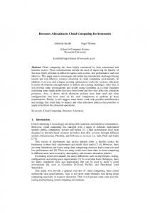
Summary of Auto-scaling Demand Index (ADI).

In order to organise workloads whose volumes resemble those of medium to large service providers, we partitioned users responsible for submitting jobs from the dataset using k-means clustering. We opted to use eight groups based on visual inspection of the results for values between 5 and 15. The algorithm receives as input vectors x1 , x2 , . . . , xn in R|T | , where xi = {r1,ui , r2,ui , . . . , r|T |,ui }, i.e., the j-th element of vector xi contains the normalized resource utilisation level of jobs submitted by user ui at time j. We employed Euclidean distance between vectors as distance metric. Finally, the number of clusters was defined in a way to have a comprehensive set of workloads with different characteristics.

Table I summarises the maximum number of machines able to meet workloads’ demand and the total number of tasks for each workload. We observe that the workloads have a fairly heterogeneous values for both number of machines and number of tasks. Figure 4 depicts the eight resulting workloads—each representing a cloud service with different CPU usage patterns. By having these workloads, we were able to perform experiments in various realistic scenarios. B. Experiment Description We conducted experiments with the workloads described earlier using several configurations, each consisting of:

•

One of the following auto-scaling triggering strategies: Reactive, Conservative, and Predictive;

•

One of the following step size configuration strategies: Adaptive and Fixed

•

An upper bound L ∈ N for the desired utilisation level, chosen from [39, 59];

•

A lower bound U ∈ N for the desired utilisation level, chosen from [60, 80];

•

Value of step size s to be used by the Fixed strategy.

We choose these intervals for L and H because they contain the values that are typically employed in practice. p m for every integer p in [1, 50], which We used s = 100 means that the tested step sizes used in the experiments represented some percentage between 1 and 50 of m, the total number of resources available in the cluster. Finally, in every configuration employing the Adaptive strategy, we used t . This represents a neutral level of α = 0.5, i.e., st = Lt +U 2 user aggressiveness. The investigation of the impact of this parameter deserves a study by itself, thus it was not considered in this article. For configurations involving the combination of the Predictive and the Adaptive strategy, the step size is defined according to the last utilisation level that has been measured, that is, according to ut . Preliminary tests that used u0t instead showed poor results, so this type of configuration was not considered in this work. In the following section, we present and analyse the results of our experiments. We consider only configurations that employ the best step sizes. More precisely, out of the 50 configurations involving Fixed (one for each step size), an auto-scaling triggering strategy, and a pair (L, U ), we chose the one delivering minimum ADI for fair comparison reasons. C. Result Analysis The results of our experiments are summarised in Figure 5. Each pair of bars in each graph is associated to the auto-scaling triggering strategy indicated in the x-axis, and the depicted values are the sum of all ADIs for every combination of L and U . Bars on the left and on the right show these sums for configurations using the Fixed and the Adaptive strategy, respectively. Finally, for better visualisation, we present the values in logarithmic scale. The comparison between strategies for setting up step sizes shows that there is no clear winner, since each provided the best results in 4 out of the 8 workloads. However, we remark that the advantage of Fixed over Active in Workloads 3 and 4 is virtually negligible. Conversely, regarding the auto-scaling triggering strategies, our results show that Reactive is consistently good, that Predictive oscillates, and that Conservative is inferior to all of them. The following paragraphs contain detailed explanations of these results and related findings.

Selecting the best step. One of the key challenges associated with the adoption of the Fixed strategy is to choose an adequate step size. Since the value does not change over time, users have to find a compromise between selecting values that are good for small changes and values that are better for large oscillations in the system utilisation. Difficulties on the selection of adequate fixed step sizes are illustrated in Figure 6, which shows the value of step size that minimises ADI for each pair (L, U ) in three workloads. The graph for Workload 4 is irregular, which is a consequence of its bursty and peaky behaviour (see Figure 4(d)). For Workload 5, we observe three values of best step, a phenomenon that can be explained by the fact that it has three intervals where variations on the utilisation level are very distinct (see Figure 4(e)). Finally, for Workload 6, there is a pattern indicating that the best step size is proportional to the size of the interval [L, U ]. Large step sizes for small intervals would generate frequent auto-scaling operations for short target utilisation intervals, such as the one depicted in Figure 3(a). These observations show that, although Fixed performs better than Adaptive in certain scenarios, the configuration of a system employing this strategy demands a certain knowledge about the characteristics of the workload. This task is specially challenging if the system utilisation suffers from irregular variations, since choosing the most adequate step size for certain periods of time may increase ADI in other intervals. Step Size Strategies. Figures 5(c), 5(d), and 5(h) show that the differences between Fixed and Adaptive in Workloads 3, 4, and 8 were marginal, and the explanation lays on their relatively “predictable” behaviour. Namely, it is reasonable to expect that, in these cases, step sizes belonging to a certain range will consistently be better than others and that the Adaptive strategy will almost always draw values for st from this range. Therefore, the step size strategy is not the most important factor in these scenarios. The Adaptive strategy was better for Workloads 1, 5, and 6 (see Figures 5(a), 5(e), and 5(f)) due to their bursty and peaky behaviours (see Figures 4(a), 4(e), and 4(f)). In these scenarios, the utilisation level changes abruptly, so Fixed needs a considerably large number of iterations before reaching the desired utilisation level (see Figure 2), whereas Adaptive resizes the resources pool immediately in order to reach the desired utilisation level. Conversely, the quick reaction of Adaptive has negative consequences if the utilisation level changes abruptly and come back to normal shortly after. The occurrence of such events explains why Fixed combined with short step sizes (see the optimal step sizes for Workload 2 in Figure 7) delivers better results for Workloads 2 and 7. Auto-scaling Triggering Strategies. Figure 5 shows that the Reactive strategy had an excellent performance in our tests. This can be explained by the fact that it always reacts immediately to any deviation from the desired utilisation interval. One can also argue that Reactive minimises ADI because it

(a) Workload 4: Irregular.

(b) Workload 5: Clustered.

Fig. 6.

(a) Reactive strategy.

Fig. 7.

(c) Workload 6: Patterned.

Different behaviours of best step depending on workload characteristics.

(b) Conservative strategy.

(c) Predictive strategy.

Optimal step sizes for Workload 2 for different triggering auto-scaling strategies.

does not sacrifice ADI in favour of some other metric, such as the number of active resources, QoS, and the number of auto-scaling operations. The Conservative strategy performed poorly in all the workloads, since it waits for the occurrence of four undesired utilisation levels in a row and only starts to react properly after suffering several ADI penalties. We remark that the results could have been more favourable to Conservative if another metric had been employed, such as the number of auto-scaling operations. Finally, the Predictive strategy was also typically worse than Reactive, but the differences were not as large as the ones involving Conservative. While the same argument used in the previous paragraph may serve to explain why Predictive is superior to Conservative, the estimation of u0t had a significant impact in the results. For Workloads 3, 4, and 8, which were the more “predictable” ones, the exponential smoothing technique delivered poor estimations and lead to several “wrong” auto-scaling operations. For the other workloads, the forecast was better and, in cases were the workload was peaky and

bursty, its results were very similar to those delivered by Reactive (e.g., Workloads 1, 2, and 6). Selection of Utilisation Interval. The performance of the auto-scaling strategies are closely related to the size of the intervals [L, U ] in several workloads. It is clear that ADI penalties increases as U −L decreases, since the interval where utilisation levels are acceptable is smaller. However, there are some intrinsic aspects from the workloads that deserve careful attention. In the case of Workload 3, we remark that the system utilisation belonged most of the time to interval [50, 80]. Figure 8(a) shows that configurations employing the Reactive strategy performed well if L ≤ 50, while those using L > 50 were considerably worse. Workload 4 presents higher variations than Workload 3, so while the same phenomenon can be observed in this case, the changes in ADI are smoother (see Figure 8(b)). Finally, the same graph for Workload 5 shows that this decay in performance applies to both step size strategies (see Figure 8(c)). This happens because there is a certain interval to which

most utilisation levels belong to. Once the interval becomes too small, ut will be very frequently out of [L, U ]. Differently from Workloads 3 and 4, we see that in Workload 5 the interval would have to be very large, and therefore the performance of both strategies (fixed and adaptive) decays with the size of the target utilisation interval. V. R ELATED W ORK Projects related to our work fall into categories of scheduling and cloud computing auto-scaling.

(a) Reactive strategy.

(b) Conservative strategy.

(c) Predictive strategy.

Fig. 8. Auto-scaling Demand Index (ADI) as a function of target utilisation interval.

Scheduling is a well-studied topic in several domains for which the number of theoretical problems, solution approaches, and practical applications is considerably large [2], [3]. Commonly used algorithms include FIFO, priority-based, deadline-driven, hybrid approaches that use backfilling techniques [4], among others [5], [6]. In addition to priorities and deadlines, other factors have been considered, such as fairness [7], energy-consumption [8], and context-awareness [9]. Moreover, utility functions were used to model how the importance of results to users varies over time [10], [11]. Related to our work is Amazon CloudWatch [12], which is a monitoring system to help deciding when Cloud resources need to be modified. In this system, users are responsible for specifying L and U and may not know how to properly setup these values. Microsoft Azure Auto-scaling system [13] also allows users to specify these auto-scaling parameters, but suffers the same limitation from Amazon platform. Scryer [14], from Netflix, is an auto-scaling engine that uses predictive models to know when resources should be added or removed. Its auto-scaling strategy is used internally by the software itself, and thus users do not interact or specify auto-scaling thresholds and policies. Ming et al. [15] proposed an architecture that deals with auto-scaling focusing on meeting user deadlines. However, it does not consider helping users to define auto-scaling thresholds and resource change steps. Shen et al. [16] presented a system to automate elastic resource scaling for cloud computing environments. Their system does not require prior knowledge about the applications running in the cloud. Other projects consider auto-scaling in different scenarios, such as auto-scaling for MapReduce applications [17], [18], vertical versus horizontal auto-scaling [19], operational costs [20], and integer model based auto-scaling [15]. A. Ali-Eldin et al. [21] introduced a tool to analyse and classify workloads and assign the most suitable auto-scale controllers based on workload characteristics. Similar to our work, A. Ali-Eldin et al. also identified the challenge aspect of developing workload predictors. Recently, we explored the use of user patience information to make better auto-scaling decisions [22]. Our study aims at enhancing existing work on auto-scaling by understanding how to define parameters for this Cloud functionality and how they impact Auto-scaling Demand Index (ADI).

VI. C ONCLUSION In this article we investigated auto-scaling strategies applied to various workload characteristics for cloud computing environments. These strategies involve the definition of when to trigger auto-scaling operations and how to modify the original resource pool depending on the workload variations over time. Our experiments utilised real-world data from a Google cluster, which contains millions of jobs that were grouped to enable the evaluation under different scenarios. The main contributions of this work are (i) the definition of Auto-scaling Demand Index (ADI) to measure the quality of auto-scaling strategies; (ii) an Adaptive strategy that configures step sizes according to the current system utilisation level; and (iii) the findings from our experiments involving two step size configuration strategies (Adaptive and Fixed) and three auto-scaling triggering strategies (Reactive, Conservative, and Predictive). The main lessons of our evaluation are: •

It is possible to use Fixed for auto-scaling when the system utilisation (or any performance metric) is regular and well-known. If workloads are irregular, bursty, and/or peaky, Adaptive delivers lower values of ADI in comparison to Fixed;

•

For peaky and bursty workloads, having a fixed step size may require a long time until the resource pool provides the target utilisation interval. This may generate a lost in QoS or a resource waste. The Adaptive strategy can then deliver more quickly the target utilisation levels. However, if, for instance, there is a short high peak, the Adaptive strategy allocates resources to meet the requirements of that peak, but at the following measurement time, it needs to reduce resources drastically again. In this case, the Fixed strategy would not go along at the same level and would deliver a satisfactory performance;

•

Predictive strategies may be interesting to help make auto-scaling decisions, but they are very much dependent on workload characteristics and precise prediction models as described by A. Ali-Eldin et al. [21]. In situations where the resource provisioning/releasing time is similar or shorter than the measurement intervals, a reactive strategy may adjust the resource pool in a more precise way because it is based on the actual and current workload information. In addition, the effects of the reactive strategy are applied quickly to adapt to the current workload demand;

•

Besides the selection of the step size and the triggering moment to execute auto-scaling operations, users still face the challenge of defining the upper and lower bounds for target system utilisation. We observed that depending on workload characteristics, certain intervals may lead

to configurations for which any auto-scaling strategy will have an unsatisfactory performance. Therefore, a recommender system to provide guidance on this aspect becomes fundamental to any cloud provider that wants to enhance user experience. We believe the findings on the investigated workloads and strategies can help cloud providers build recommender systems for auto-scaling operations. R EFERENCES [1] “Google cluster-usage traces: format + schema,” 2013. [Online]. Available: https://code.google.com/p/ googleclusterdata/ [2] J. Blazewicz, K. Ecke, G. Schmidt, and J. Weglarz, Scheduling in Computer and Manufacturing Systems, 2nd ed., 1994. [3] M. L. Pinedo, Planning and Scheduling in Manufacturing and Services, 2nd ed., 2007. [4] D. Tsafrir, Y. Etsion, and D. G. Feitelson, “Backfilling using system-generated predictions rather than user runtime estimates,” IEEE Transactions on Parallel and Distributed Systems, vol. 18, no. 6, pp. 789–803, 2007. [5] T. D. Braun et al., “A comparison of eleven static heuristics for mapping a class of independent tasks onto heterogeneous distributed computing systems,” Journal of Parallel and Distributed computing, 2001. [6] D. G. Feitelson, L. Rudolph, U. Schwiegelshohn, K. C. Sevcik, and P. Wong, “Theory and practice in parallel job scheduling,” in Proc. of the Workshop on Job Scheduling Strategies for Parallel Processing (JSSPP’97), 1997. [7] N. D. Doulamis, A. D. Doulamis, E. A. Varvarigos, and T. A. Varvarigou, “Fair scheduling algorithms in grids,” IEEE Transactions on Parallel and Distributed Systems, 2007. [8] J.-F. Pineau, Y. Robert, and F. Vivien, “Energy-aware scheduling of bag-of-tasks applications on master– worker platforms,” Concurrency and Computation: Practice and Experience, vol. 23, no. 2, pp. 145–157, 2011. [9] M. D. Assunc¸a˜ o et al., “Context-aware job scheduling for cloud computing environments,” in Proc. of the IEEE Int. Conf. on Utility and Cloud Computing (UCC), 2012. [10] C. B. Lee and A. Snavely, “Precise and realistic utility functions for user-centric performance analysis of schedulers,” in Proc. of the Int. Symp. on High-Performance Distributed Computing (HPDC’07), 2007. [11] A. AuYoung et al., “Service contracts and aggregate utility functions,” in Proc. of the 15th IEEE Int. Symp. on High Performance Distributed Computing (HPDC’06), 2006. [12] “Amazon CloudWatch,” 2014. [Online]. Available: http://docs.aws.amazon.com/AWSEC2/latest/ UserGuide/using-cloudwatch.html [13] “Microsoft Azure,” 2014. [Online]. Available: http://www.windowsazure.com/en-us/documentation/ articles/cloud-services-how-to-scale/

[14] “Scryer: Netfix’s Predictive Auto Scaling Engine,” 2014. [Online]. Available: http://techblog.netflix.com/2013/12/ scryer-netflixs-predictive-auto-scaling.html [15] M. Mao, J. Li, and M. Humphrey, “Cloud auto-scaling with deadline and budget constraints,” in Proc. of the 11th IEEE/ACM International Conference on Grid Computing (GRID). IEEE/ACM, 2010, pp. 41–48. [16] Z. Shen, S. Subbiah, X. Gu, and J. Wilkes, “Cloudscale: elastic resource scaling for multi-tenant cloud systems,” in Proc. of the 2nd ACM Symposium on Cloud Computing. ACM, 2011, p. 5. [17] Y. Chen, S. Alspaugh, and R. Katz, “Interactive analytical processing in big data systems: A cross-industry study of mapreduce workloads,” Proc. VLDB Endow., 2012. [18] Z. Fadika and M. Govindaraju, “DELMA: Dynamically ELastic MapReduce Framework for CPU-Intensive Applications,” in Proc. of the 11th IEEE/ACM International Symposium on Cluster, Cloud and Grid Computing (CCGrid’11), 2011, pp. 454–463.

[19] M. Sedaghat, F. Hernandez-Rodriguez, and E. Elmroth, “A virtual machine re-packing approach to the horizontal vs. vertical elasticity trade-off for cloud autoscaling,” in Proc. of the ACM Cloud and Autonomic Computing Conference (CAC’13). ACM, 2013. [20] M. Mao and M. Humphrey, “Auto-scaling to minimize cost and meet application deadlines in cloud workflows,” in Proc. of the Int. Conf. for High Performance Computing, Networking, Storage and Analysis (SC), 2011. [21] A. Ali-Eldin, J. Tordsson, E. Elmroth, , and M. Kihl, “Workload classication for ecient autoscaling of cloud resources,” Technical Report, 2005. [Online]. Available: http://www8.cs.umu.se/research/ uminf/reports/2013/013/part1.pdf [22] R. L. F. Cunha, M. D. Assunc¸a˜ o, C. Cardonha, and M. A. S. Netto, “Exploiting user patience for scaling resource capacity in cloud services,” in Proc. of the 7th IEEE International Conference on Cloud Computing (CLOUD’14), 2014.