task of distinguishing whether an image blob is a vehicle, a single human, a ... [2] have proposed a binary classification method which uses two feature vectors ...
Evaluating Feature Importance for Object Classification in Visual Surveillance Masamitsu Tsuchiya, Hironobu Fujiyoshi Dept. of Computer Science, Chubu University Aichi 487-8501 Japan {tsuchiya, hf}@vision.cs.chubu.ac.jp Abstract Feature-based object classification, which distinguish a moving object to human or vehicle, is important in visual surveillance. In order to improve classification performance, in addition to choosing between the classification (such as SVM, ANN etc), we have to pay attention to which subset of features to employ in the classifier. This paper describes a method to evaluate the relative importance of various features for object type classification. Starting with a given set of features, we apply the AdaBoost method and then we compute a metric which enables us to choose a good subset of the features. We apply our method to the task of distinguishing whether an image blob is a vehicle, a single human, a human group, or a bike, and we determine that shape-based feature, texture-based feature, and motion-based feature are reliable for this classification task. We validate our method by comparing with performance of ANN-based classification.
1
Introduction
Feature-based methods are commonly used for object recognition and type classification in visual surveillance[1]. For robustness, we need to select features that are invariance to various changes caused by environment, scaling, viewpoint, and lighting. In order to improve classification performance, in addition to choosing between the classifier (such as SVM, ANN, and etc.), we have to pay attention to which subset of features to employ in the classifier. Especially, in outdoor surveillance, we have to carefully design good features for input vectors of the classifier. Previous work in this area has focused on producing descriptors and classification method that are invariant to scaling and viewpoint of the detected objects. Lipton et. al [2] have proposed a binary classification method which uses two feature vectors, e.g., dispersedness and area, to distinguish the image blob detected by the adaptive background detection. The automated video surveillance system called
VSAM[1] uses artificial neural network(hereafter referred to as ANN) based classification which enables classification robust to size changes (by using information about the zoom parameter of camera). Since both these features are only shape-based features, the performance is not high. Texture-based features such as histograms of oriented gradients for human detection have been proposed[3]. They compute high dimensional features based on edges and use SVM (binary classification) to detect human regions. Viola and Jones have proposed a pedestrian detection system that integrates intensity information with motion information[4]. Although the systems are aimed for human detection, these methods can be applied to multi-class classification. However, in these methods, the relative contribution of features is not considered because it is difficult to measure how effective each feature vector is. Further, a common problem in using a learning based classifier such as ANN is that they act essentially as a black box that performs the assigned task for the user. Additionally, if we have too many training sets, it is hard to make a desired combination of feature sets. This paper describes a method to evaluate the relative importance of features for object type classification. Starting with a given set of features, we apply the AdaBoost method and then we compute a metric which enables us to choose a good subset of the features. We apply our method to the task of distinguishing whether an image blob is a vehicle (hereafter referred as VH), a single human (SG), a human group (HG), or a bike (BK), and we determine that shape-based feature, texture-based feature, and motion-based feature are reliable for this classification task.
2
Features
We use temporal differencing to detect moving objects and for each detected region, we compute feature vectors for object type classification. To classify objects in a video stream, it is important to use a classification metric which is computationally inexpensive, reasonably effective for small numbers of pixels on object, and invariant to lighting con-
verticlal
ditions or viewpoint. This study introduces three different kinds of features, viz., shape-based feature, texture-based feature, and motion-based feature.
2.1
horizontal
left-up
right-up
Shape-based Feature
(1) Aspect ratio Aspect ratio is determined relative size to measure two extensions of the object. We apply ellipse fitting onto detected regions as shown in Figure 1. Aspect ratio =
(a) VH
length of minor axis . length of major axis
(b) SH
(c) HG
(1)
(b) SH
2.3
Motion-based Feature
(4) Variance of optical flow vectors A moving vehicle gives rigid motion and a walking human gives non-rigid motion. In order to measure the rigidity of the motion for a moving object, we employ variances of optical flow distribution for 6 blocks. Figure 3 shows examples of optical flow vectors for each category obtained by the KLT method[5]. Given the histogram of the optical flow vectors
(d) BK
Figure 1. Examples of aspect ratio (2) Complexity of shape the complexity of shape,
(a) VH
Figure 2. Examples of edge information
Dispersedness is a measure of
Dispersedness =
P erimeter2 . Area
(2)
(a) VH
(b) SH
(c) HG
(d) BK
Figure 3. Examples of optical flow vector
A human blob, having a more complex shape, tend to have larger dispersedness than a vehicle blob.
2.2
Texture-based Feature
(3) Edge magnitude and connectivity (8-dimensional vector) The gradient magnitude g(x, y) and the gradient direction θ(x, y) are computed for each pixel using equation (3). 1
2 + IY2 ) 2 , θ(x, y) = atan( g(x, y) = (IX
IY ) IX
(3)
The simplest implementation of this would be to convolve the 3 × 3 mask with the image, aligning the mask with the x and y axes to compute the values of Ix and Iy . The gradient direction is divided into four directions such as horizontal, vertical, right-up, and left-up directions as shown in Figure 2. We collect all the pixels which have the same direction (only the four directions) and we compute the normalized sum of their gradient magnitude to get four values. Connectivity of edge segment for each direction is computed by counting the number of edges which share the same direction and are connected to each other. These four values along with the previous 4 values give us the 8 dimensional texture-based vector.
Figure 4. Variance of optical flow vector of a moving object as shown in Figure 4(a), the moving direction θ is selected as median of the histogram. Variances of each region σi are computed as shown in Figure 4(b). The least-square method is applied to compute the gradient of the variance by the following equation, G=
n
�n �n xi σi − i=1 xi i=1 σi �n � 2 n n i=1 x2i − ( i=1 xi )
�n
i=1
(4)
where n = 6 in this study. The gradient value G nearly equals to 1 for rigid motion. The above mentioned 11 features are normalized to be between 0 to 1.
3
Evaluating the Relative Contribution of Features
We use the AdaBoost method to construct a binary classifier for each category, and then we compute a metric which evaluates importance of the feature.
3.1
4.
Dataset
We collected 200 learning sample images for each category (VH, SH, HG, BK) from a video database of 23 hours. So, total of 800 images is used for training the AdaBoost classifier. A human operator collects sample image and assign class labels to them. Another 800 images are used in the discriminant experiments described in section 4.
3.2
Training Process and Discrimination
In this paper, the training process of AdaBoost is used to obtain a metric for evaluating the contribution of a feature, not used as a classifier. In training process, Adaboost selects a subset of features in order to construct a robust classifier from training dataset {(xi , yi ) : 1 < i < n} where x = (x1 , · · · xP ) is 11dimensional feature vector and y ∈ {−1, +1} is class label. For example, y is set by the following equation in the case of training the VH Classifier. � +1, if xi ∈ V H yi = (5) −1, otherwise In this implementation, n is 800 (200 positive examples plus 600 negative examples). In each round, the learning algorithm chooses from the 11 features described in section 2. The AdaBoost algorithm picks the optimal threshold th for each feature p by the following equation. � (x) =(0 argmin { I(yi = sgn (xpi − th))} hp,th t ≤ th ≤ 1 , 1 ≤ p ≤ P ) i
(6) The output of the Adaboost after the learning process is a binary classifier that consists of a linear combination of the selected features with weighs αt . Therefore, the final classifer HT is given by the following equation, HT (x) =
1. 2. 3.
T �
αt h(t) (x).
(7)
t=1
The AdaBoost algorithm is given below. We trained four classifiers one for each class (VH, SH, HG, BK) using the method described above.
Algorithm The Adaboost algorithm Input: n, Training dataset (xi , yi ) · · n), h0 (x) = 0 Initialize: w1 (i) = 1/n(i = 1 ·� n Do for t = 1, . . . , T. �t (h) = i I(yi �= h(xi ))wt (i) (a) �t (h(t) ) = min�t (h) 1−�t (h(t) ) (b) αt = 12 ln( �t (h ) (t) ) (c) wt+1 (i) = wt (i) exp(−αt h(t) (xi )yi )) Output: Final hypothesis with weights αt T � sign(Ht (x)), where HT (x) = αt ht (x) t=1
In the discriminant process, we have to merge the results of four trained classifiers as a multi-class classification. The final decision is made by searching the maximum value of the outputs obtained by each classifier H c () for the category c using normalized weights αt� .
H c (x) = Class = c argmax ∈ {V H, SG, HG, BK}
T �
αt� ht(x) (8)
t=1
where the normalized weights is obtained by αt� = .
3.3
� Tαt
i=0
αi
Contribution of Feature
Each round of Adaboost chooses from the total set of the various features, the feature with lowest weighted error on the training examples. The final classifier balances the 11 features in order to maximize classification performance. The weight α, the selected feature, and the thereshold th are chosen at each round are very important factors for classification performance. This introduces a metric which indicates how well the features “contribute” to the classification performance. We define a contribution ratio Cp for each feature p by the following equation,
Cp =
T �
αt� · δK [P (ht ) − p]
(9)
t=1
where p is a kind of feature, and P () is a function to output the feature chosen at round t in the AdaBoost training process, let δK be Kronecker delta. This contribution ratio Cp becomes a metric to measure the contribution of the feature vector p. This enables us to determine which subset of the features should be chosen in a given classification task.
Error rate
Contribution rate
Error rate[%] 0.004
50
Error rate[%]
Error rate[%] 40
30
Error rate[%]
0.12
30 0.07
0.002
20 0.001
10 0
0
AS
CS
V
H
R-U
L-U
OF
(a) Vehiccle(VH)
R= 0.74 0.1
20 0.08
15 10 5
AS
CS
V
H
R-U
L-U
0.08 0.06
10
0.04
0
0.06
20
0.05
10 0.04
0.04 0.02
AS
(b) Single human(SH)
R= 0.85
0.1
20
0.06
OF
R= 0.83
30
Contribution[%]
30
25 Contribution[%]
Contribution[%]
0.003
Contribution[%]
0.12
R= 0.50
40
CS
V
H
R-U
L-U
(c) Human group(HG)
OF
0
0.03
AS
CS
V
H
R-U
L-U
OF
(d) Bike(BK)
AS:Aspect Ratio, CS:Complexitiy of Sahpe, V:Vertical edge, H:Horizontal edge, R-U:Right-up edge, L-U:Left-up edge V , OF:ariance of Optical Flow
Figure 5. Contribution ratio and error ratio
4
Experiment
4.1
Contribution Ratio
Figure 5 shows the contribution rate Cp of feature vector p and the error rate in the discriminant experiments using ANN when it is trained without the feature p. We tested ANN-based classification with 200 sample images for each class, which are not contained in the training sets. Table 1 shows a confusion matrix of the ANN-based classification results. The R in the figure denotes a correlation coefficient between them. This is a measure of how well the contribution ratio “fits” with the classification performance. It is clear that there is a strong correlation between the contribution ratio and the classification performance except vehicle class (VH). This is due to the fact that the “vertical”, “horizontal”, “right-up”, and “left-up” features work in a complementary manner.
In
4.2
Table 1. Classification results by ANN Out VH SH HG BK correct [%] VH 200 0 0 0 200 100.0 SH 0 181 11 8 181 90.5 HG 0 6 189 5 189 94.5 BK 3 7 0 190 190 95.0 Sum 760 95.0
Selected Features
From the Figure 5, we make the following observations about the features for object type classification. For vehicle class(VH), we see that the edge information , especially horizontal component, is effective as a feature for the classification. On the other hand, for other categories, i.e., single human class (SH), human group class (HG), bike class (BK), the shape-based feature such as aspect ratio and complexity of the shape as well as texture-based features are important. For bike class, the motion-based feature such as
a variance of optical flow vectors is also important to distinguish a single human class and a bike class. Although the appearances of single human and bike can be very similar from some viewpoints, the motion-based feature distinguishes between the walking human’s non-rigid motion and the bike’s rigid motion.
5
Conclusion
This paper presents a metric, contribution ratio, to evaluate how important a feature is for the task of object type classification. The contribution ratio is obtained from the selected features and weights in the AdaBoost training. The ratio is experimentally validated by demonstrating positive correlation with the performance of a ANN-based method. This helps us to find which feature should be chosen, in a general learning-based classifier.
References [1] R. Collins, A. Lipton, H. Fujiyoshi, and T. Kanade, “Algorithms for cooperative multisensor surveillance,” Proc. of the IEEE, Vol. 89, No. 10, October, 2001, pp. 1456 - 1477. [2] A. Lipton, H. Fujiyoshi, and R.S. Patil. “Moving target detection and classification from real-time video.” Proc. of the 1998 Workshop on Applications of Computer Vision, 1998. [3] N. Dalal and B. Triggs, “Histograms of oriented gradients for human detection,” In Proc. of the IEEE Conference on Computer Vision and Pattern Recognition, San Diego, CA, pp.886-893, 2005 [4] P. Viola, M. J. Jones, D. Snow. “Detecting Pedestrians Using Patterns of Motion and Appearance,” Proc. of the Ninth IEEE International Conference on Computer Vision (ICCV’03) Volume 2, 2003. [5] B. D. Lucas and T. Kanade., “An Iterative Image Registration Technique with an Application to Stereo Vision.” International Joint Conference on Artificial Intelligence, pp. 674679, 1981.