Oct 7, 2010 - and Faluvegi, 2009; Shindell et al., 2008; Stier et al.,. 2006]. These studies typically examined the response to aerosol forcing. However, as ...
Oct 7, 2010 - Dufresne et al. [2005],. Hourdin et al. [2006] ..... IPSL infrastructure Pole de modelisation, led by JeanâLouis Dufresne and Pascale Braconnot.
Australia and â Australian Rivers Institute, Griffith University,. Nathan ..... salt barriers (Musyl & Keenan, 1992; Jerry, 1997; Wong et al., 2004) and inter-.
interactions of CO 2-saturated brine with the Eau Claire Shale. Geochemical .... Illinois and southern Wisconsin (outside the basin) and is used to store industrial ...
Dec 22, 2014 - JENNIFER N. HARDING| AND JOHN D. REYNOLDS. Earth to Ocean Research Group, ...... Perry, and W. B. Taliaferro. 1989. Shredders and.
Aug 15, 2018 - et al., 2000), and fishes, the focus of this review, compose the greatest ...... in. g h o o k size to n o n. -ta rg e t fish size a n. d u sin. g c e rta in h o o k ty p e ..... species in both troll and longline fisheries (reviewed i
habitat, and coral recruitment patterns can drive .... vidual (recruit) was circled with an indelible pen, num- bered ... unpublished data) to estimate the density of adult popula- ..... recovery through transplantation and natural recruitment, Kenya
lateral bud release shortly following apex decapitation of chickpea. (Cicer arietinum) seedlings. Johanna C. Madera R. J. Neil Emeryb,* and Colin G N. Turnbullc.
emergency triage centerâ into the community's EMS ... their members to call the gate- keeper prior to 9-1-1. ... vices; EMS; ambulance; 911; man- aged care ...
Feb 28, 2008 - the UK. This review looks at the recent history of the ..... gram (EEG)52â54 or evoked potentials, neuroradiological tech- ... Orlando, Florida:.
Nov 14, 2017 - 1The Aerospace Corporation, El Segundo, CA, USA, 2Laboratory for ...... Ergun, R. E., Tucker, S., Westfall, J., Goodrich, K. A., Malaspina, D. M., ...
Durie BGM, Harousseau J-L, Miguel JS, et al. International uniform response criteria for multiple myeloma. Leukemia 2006
standard statistical software programs such as SAS. (SAS Institute, Cary, North ... ysis despite having censored data, while also accounting for the uncertainty ...
Diagnosis: The diagnosis requires (1) 10% or more clonal plasma cells on bone marrow examination or a bi- ...... Demo SD
markets and appreciating markets as social constructs, which are governed by institutions ... Keywords: Economic sociology; Markets; Institutions; Food quality; ...
Mar 1, 2011 - March 2011 Dialysis & Transplantation 133. Dialysis is ... Internal ValidityâThe degree to ... What every patient care technician needs to know ...
Ian G. J. Dawson, Johnnie E. V. Johnson,. â and Michelle A. Luke. Accumulating evidence shows that certain hazard combinations interact to present synergistic.
Jul 27, 2017 - Abstract. The resurrection approach of reviving ancestors from stored propagules and compar- ing them with descendants under common ...
of statistical and analytical tools linked to phylogenetic reconstructions allowed researchers to deepen our knowledge of patterns and processes in rotifer ...
With this issue, Aging Medicine launches as the official English-lan- guage journal of the Chinese Geriatrics Society. Dr. Jian-ye Wang and I are honored to be ...
and Fishbein's theory of reasoned action in order to understand public support for building a dam to meet local water supply needs. Methods. The linkages ...
Saunders, 1994; Yates & Hobbs, 1997a; de Blois et al., 2001,. 2002). The analogy between remnant patches in agricultural. The Johnstone Centre, Charles Sturt.
John J. Wheeler1, Michael R. Mayton2, Julie Ton4 and Joshua E. Reese3 .... ment agent categories were replicated from McIntyre et al. (2007). TI was evaluated ...
Endowed Chair Award, which was used to fund this project. ...... and taking medicines. Brit Med J. ... Research Service. Rural economy and population, 2017.
Feb 7, 2017 - Lara G. Melchior1 | Denise de C. Rossa-Feres2 | Fernando R. da Silva3 ..... Core Team, 2014) using the âbetapartâ (Baselga, Orme, Villeger, De.
|
|
Received: 9 November 2016 Revised: 27 January 2017 Accepted: 7 February 2017 DOI: 10.1002/ece3.2852
ORIGINAL RESEARCH
Evaluating multiple spatial scales to understand the distribution of anuran beta diversity in the Brazilian Atlantic Forest Lara G. Melchior1 | Denise de C. Rossa-Feres2 | Fernando R. da Silva3 1
Programa de Pós Graduação em Biologia Animal, Universidade Estadual Paulista Júlio de Mesquita Filho – UNESP, São José do Rio Preto, São Paulo, Brazil 2
Departamento de Zoologia e Botânica, Universidade Estadual Paulista Júlio de Mesquita Filho – UNESP, São José do Rio Preto, São Paulo, Brazil 3 Laboratório de Ecologia Teórica: Integrando Tempo, Biologia e Espaço (LET.IT.BE), Departamento de Ciências Ambientais, Universidade Federal de São Carlos – UFSCar, Sorocaba, São Paulo, Brazil
Correspondence Fernando R. da Silva, Departamento de Ciências Ambientais, Universidade Federal de São Carlos – UFSCar, Sorocaba, SP, Brazil. Email: [email protected] Funding information Fundação de Amparo à Pesquisa do Estado de São Paulo, Grant/Award Number: 2010/52321-7 and 2013/50714-0; Coordenação de Aperfeiçoamento de Pessoal de Nível Superior (CAPES); Conselho Nacional de Desenvolvimento Científico e Tecnológico, Grant/Award Number: 303522/2013-5 and 563075/2010-4
Abstract We partitioned the total beta diversity in the species composition of anuran tadpoles to evaluate if species replacement and nestedness components are congruent at different spatial resolutions in the Brazilian Atlantic Forest. We alternated the sampling grain and extent of the study area (among ponds at a site, among ponds within regions, among sites within regions, and among sites within regions pooled together) to assess the importance of anuran beta diversity components. We then performed variation partitioning to evaluate the congruence of environmental descriptors and geographical distance in explaining the spatial distribution of the species replacement and nestedness components. We found that species replacement was the main component of beta diversity, independent of the sampling grain and extent. Furthermore, when considering the same sampling grain and increasing the extent, the values of species replacement increased. On the other hand, when considering the same extent and increasing the sampling grain, the values of species replacement decreased. At the smallest sampling grain and extent, the environmental descriptors and geographic distance were not congruent and alternated in the percentage of variation explaining the spatial distribution of species replacement and nestedness. At the largest spatial scales (SSs), the biogeographical regions showed higher values of the percentage explaining the variation in the beta diversity components. We found high values of species replacement independently of the spatial resolution, but the processes driving community assembly seem to be dependent on the SS. At small scales, both stochastic and deterministic factors might be important processes structuring anuran tadpole assemblages. On the other hand, at a large spatial grain and extent, the processes restricting species distributions might be more effective for drawing inferences regarding the variation in anuran beta diversity in different regions of the Brazilian Atlantic Forest. KEYWORDS
dispersal limitation, environmental heterogeneity, nestedness, species replacement, stochasticity, tadpoles
1 | INTRODUCTION
number of species by site, and beta diversity (β) that is the variation in the species identities from site to site (Whittaker, 1960, 1972). The concepts
Total species richness of a region, frequently named gamma diversity
of beta diversity and species turnover have often been used interchange-
(γ), can be partitioned in two components: alpha diversity (α) that is the
ably in the ecological literature; however, the failure to recognize the
F I G U R E 1 (a) Original Brazilian Atlantic Forest distribution and the 12 sites evaluated in this study. Forest types are indicated by different shades of gray (light gray—semideciduous seasonal forest—SSF, gray—dense rain forest—DRF, and dark gray—mixed rain forest—MRF). Ubatuba (UBA) is highlighted illustrating that different ponds were sampled within sites. (b) Schematic representation of the different spatial scales addressed in this study. Arrows with solid lines consider ponds as the sampling units and the sites (SS1) or the forest types (SS2) separately as the extent. Arrows with dashed lines consider sites as the sampling units and the forest types separately (SS3) or the three forest types pooled together (SS4) as the extent. Circles represent sites, hexagons represent each region separately, and rectangle represents regions pooled. Details of the sites are in Appendix S1 distinction between these terms can lead to the inappropriate use of some
Although it is recognized that the spatial distribution of beta diversity is
beta diversity indices (Anderson et al., 2011; Koleff, Gaston, & Lennon,
related to processes and mechanisms operating at different spatial scales
2003). Recently, Baselga (2012) partitioned the total beta diversity into
ent considering similar SSs within and among regions of the Brazilian
Furthermore, each pond contains fewer species than the total spe-
Atlantic Forest (Figure 2a). This approach will help us to understand if
cies richness observed in sites, indicating that ponds differ in spe-
distribution patterns of beta diversity obtained in one study apply only
cies composition (see Table S1 in Appendix S1). Based on these facts
to the area under investigation or whether they can emerge on other
and considering that the smaller the grain, the greater the dissimi-
communities considering similar SSs (Lawton, 1999). Our second objec-
larity among the sampling units (Nekola & White, 1999), we predict
tive was to understand if ecological processes such as species sorting
high values of species replacement among ponds because of the
and dispersal limitation are congruent within and among different re-
variation in stochastic factors such as recruitment or random coloni-
gions considering similar spatial grains and extents. To this, we evalu-
zation (Chase, 2007; Hubbell, 2001). If the values of species replace-
ated four different SSs across the Brazilian Atlantic Forest (Figure 1):
ment are similar among sites, we expect that all sites will present higher values of species replacement than nestedness (Figure 2a), in
SS1) Beta diversity among ponds within each site (smallest spatial
all regions sampled. Furthermore, if stochastic factors are the main
grain and extent): At small grain, both stochastic species occupancy
drivers of the species replacement, we expect no association with
F I G U R E 2 Illustration of the hypotheses evaluated in this study. (a) Three scenarios for the distribution of species replacement (βjtu) and nestedness (βjne) values considering ponds as sampling unit and sites as extent (SS1): (i) Species replacement is the main beta diversity component in the three sites and dissimilarity values are similar among sites; (ii) species replacement is the main beta diversity component in the three sites, but dissimilarity values are different among sites; (iii) species replacement and nestedness values are dependent on the site and dissimilarity values are different among sites. For illustrative purpose we showed SS1, but it can be applied to all spatial scales. (b) Predictions of the relative importance of environmental variables and geographical distance explaining variation in anuran community composition at different spatial scales. Please see text to details of the predictions
|
MELCHIOR et al.
4
environmental descriptors or geographic distance (Figure 2b); SS2) Beta diversity among ponds within each region (smallest spatial
temperatures (averages from 15 to 25°C), which influence floristic distributions (Oliveira-Filho & Fontes, 2000). According to Oliveira-Filho
grain and intermediate extent): Compared to SS1, we increased the
and Fontes (2000), the south and southeast Brazilian Atlantic Forest
extent from sites to regions. Because we increased the regional
can be classified into three forest types: (1) dense rain forest (hereafter
species pool when the extent was increased (Harrison & Cornell,
DRF)—this forest is associated with the Atlantic coast, with elevations
2008), we predict that the values of species replacement among
ranging from 50 to 2,200 m a.s.l. It occurs in climates with high and con-
the ponds will be higher than the values observed in SS1 (Barton
stant rainfall throughout the year that ranges from 2,000 to 3,600 mm
et al., 2013). Because community similarity decays with distance
(Oliveira-Filho & Fontes, 2000). The annual mean temperature (AMT)
(Nekola & White, 1999), we expect that geographic distance will
varies between 22 and 25°C (Colombo & Joly, 2010); (2) semidecidu-
have a greater relative importance in determining the spatial distri-
ous seasonal forest (SSF)—this forest is associated with inland areas
bution of species replacement than local environmental descriptors
with elevations below 700 m a.s.l. It occurs in climates with a prolonged
(Tuomisto, Ruokolainen, & Yli-Halla, 2003; Figure 2b); SS3) Beta diversity among sites within each region (intermediate spa-
dry season (from 2 to 6 months—from April to September). SSF has an annual rainfall that ranges from 1,500 to 2,000 mm (Oliveira-Filho &
tial grain and intermediate extent): Compared to SS2, we increased
Fontes, 2000) and an AMT that varies between 22 and 25°C (Colombo
the grain from ponds to sites. An increase in the grain generally de-
& Joly, 2010); and (3) mixed rain forest (MRF)—this forest occurs in the
creases the dissimilarity among the sample units because a greater
southern Atlantic Forest, with a northern distribution limit in the Serra da
proportion of the spatial heterogeneity of the system is contained
Mantiqueira (latitude 20°S) at elevations above 500 m a.s.l. It occurs in
within the grain (Barton et al., 2013; Wiens, 1989). Thus, the re-
areas subjected to tropical and sub-tropical humid climates without pro-
gional species pool is similar to that of SS2, but we increased the
nounced dry periods. MRF has an annual rainfall that ranges from 1,400
number of species within a single sample unit (Nekola & White,
to 2,200 mm and temperatures that vary from 12 to 18°C (Colombo &
1999; Wiens, 1989). Because sites within the same region are in-
fluenced by similar climatic conditions and regional species pool
Silva, Seger, and Marques (2014) found that MRF contain different
(da Silva, Almeida-Neto, Prado, Haddad, & Rossa-Feres, 2012), we
lineages when compared to DRF and SSF likely resulting from the bio-
predict that the differences in species composition among the sites
geographical origin of several taxa occurring in these forests. According
will be due to turnover of rare anuran species. Therefore, we expect
to these authors, MRF are related to conifers, while DRF and SSF are
higher values of species replacement than nestedness;
related to Myrtales and fabids, respectively. The vegetation types of the
SS4) Beta diversity among sites among the three regions pooled to-
Atlantic Forest (Oliveira-Filho & Fontes, 2000) are congruent with re-
gether (intermediate spatial grain and largest extent): Compared to
gions based on anuran species composition proposed by Vasconcelos
SS3, we increased the extent from each region to the regions pooled
et al. (2014). Therefore, for this study we considered the names of veg-
together. An increase in the extent generally increases the dissimi-
etation formations (SSF, DRF, and MRF) for the broadest scale (Figure 1).
larity among the sample units by including different biogeographical areas (Wiens, 1989). At this large spatial extent, the variation in species is associated with historical and evolutionary events (e.g., speciation and extinction), geographical barriers, and environmental filters
2.2 | Anuran tadpole data and spatial scales We compiled distributional records of tadpole assemblages (presence
(Harrison & Cornell, 2008; Svenning et al., 2011). Because regions
and absence data) from literature and data from the project SISBIOTA
contain different regional species pools (Vasconcelos et al., 2014),
CNPq/FAPESP Brazilian Tadpole Biology (coordinate by Denise C.
we predict that the values of species replacement will be lower
Rossa-Feres). These studies were carried out with standardized sur-
among sites within the same region than among those of different
veys across the DRF, SSF, and MRF regions in the Brazilian Atlantic
regions. Therefore, we expect that the values of species replacement
Forest. We limited our study to three of the four regions proposed by
will be associated with the region in which sites are located due to
Vasconcelos et al. (2014) because there are no checklists of tadpole as-
semblages that encompass the northeastern Brazilian Atlantic Forest. To
Neto, & Arena, 2014; da Silva, Almeida-Neto, et al., 2012).
reduce potential bias, we selected only studies that (1) sampled tadpoles with a wire mesh dip net; (2) carried out the surveys during the rainy season, which is the reproductive period of most anuran species, and (3)
2 | MATERIALS AND METHODS 2.1 | Study area
carried out the surveys in ponds, puddles, or marshes (hereafter ponds), excluding streams and other lotic systems. We obtained tadpole assemblages for 102 ponds (38 in SSF, 41 in DRF, and 23 in MRF) distributed across 12 sites (see Table S1 in Appendix S1; Figure 1). Overall, we gath-
The Brazilian Atlantic Forest hotspot is one of the most diverse biomes
ered 96 anuran species with SSF, MRF, and DRF regions harbored 32,
in the world (Mittermeier, Myers, Mittermeier, & Robles Gil, 2005). Its
34, and 52 species, respectively, and four anuran species occurred in all
broad geographical variation ranging from latitudes of 6°N to 30°S and
three regions (see Table S2 in Appendix S1).
longitudes of 35°W to 52°W results in a climatic gradient related to the
Based on these data, we used different spatial grains (i.e., ponds and
annual rainfall (from approximately 800–4,000 mm) and mean annual
sites) and extents (i.e., sites, each region separately, and regions pooled
|
5
MELCHIOR et al.
together) across the Brazilian Atlantic Forest to evaluate the congruence in the distribution of beta diversity considering four SSs (Figure 1).
linear models, with a Gaussian distribution and the log link function (Figure 2a). For SS1, we compared if dissimilarity values between ponds are similar within each region. For SS2 and SS3, we compared
2.3 | Environmental descriptors of sampling units
if dissimilarity values of ponds (SS2) or sites (SS3) are similar among regions. When the dissimilarity values were different within or among
The environmental descriptors of the ponds were obtained from origi-
regions, we compared the treatments using a post hoc Tukey test. We
nal studies (see Table S1 in Appendix S1). They were selected based on
inspected the data graphically (e.g., q–q plots), and when necessary,
preview studies that demonstrated the importance of these descriptors
prior to the analyses the data were log-transformed to achieve nor-
for the species richness and composition of anurans (da Silva, Gibbs,
mality and homoscedasticity.
et al., 2012; Hecnar & M’Closkey, 1998; Van Buskirk, 2005). The environmental descriptors selected were (1) hydroperiod: classified as permanent or temporary; (2) pond area: considering the maximum pond width and length (in m2); (3) maximum depth (in meters); (4) pond location: inside forest, at forest edge, or open area; (5) number of vegetation types on the pond margins; and (6) number of vegetation types in the
2.4.3 | Relative importance of geographical distance and environmental descriptors in explaining the variation in beta diversity components We reduced the multicollinearity among the environmental descrip-
interior of the pond: Both were scored as one of four categories: (1) no
tors of the sites using principal component analysis (PCA). We then
vegetation, (2) only herbaceous vegetation, (3) herbaceous vegetation
used the first two axes of the PCA (corresponding to 89% of the total
and shrubs or trees, and (4) herbaceous vegetation, shrubs, and trees.
variance) as the environmental descriptors in the analysis. The relative
The climatic descriptors of the sites were extracted from the
importance of geographical distance (Euclidean distance, representing
WorldClim database (Hijmans, Cameron, Parra, Jones, & Jarvis, 2005) at
the decay in similarity among the sampling units with distance; Nekola
a resolution of 2.5′ through DivaGIS 7.5 software. These variables were
& White, 1999) and the environmental descriptors was calculated
chosen because they describe the central tendency as well as the variation
using variation partitioning analysis (Borcard, Legendre, & Drapeau,
in the temperature and precipitation and therefore represent the physio-
1992). This approach partitions the total percentage of variation into
logical limits of amphibians (Buckley & Jetz, 2008; da Silva, Almeida-Neto,
unique and shared contributions of the sets of predictors. The total
et al., 2012): (1) the AMT; (2) the maximum temperature of the warm-
variation in the pairwise beta diversity components from hypotheses
est month (MTWM); (3) the minimum temperature of the coldest month
SS1, SS2, and SS3 was divided into four fractions: (1) the variation
(MTCM); (4) the difference between the MTWM and MTCM; (5) the an-
explained purely by geographical distance; (2) the variation explained
nual precipitation; (6) the precipitation seasonality; (7) the precipitation
purely by environmental descriptors; (3) the shared variation ex-
of the wettest quarter (PRWQ); (8) the precipitation of the driest quarter
plained by environmental descriptors and geographical distance; and
(PRDQ); and (9) the difference between the PRWQ and PRDQ.
(4) unexplained variation (residual). The total variation in the pairwise beta diversity components from SS4 was divided into eight fractions.
2.4 | Data analysis 2.4.1 | Beta diversity components
The first four are identical to the previous fractions, and the other four include (5) the variation explained purely by regions; (6) the shared variation explained by environmental descriptors and regions; (7) the shared variation explained by geographic distance and regions;
We calculated the dissimilarity in species composition between the
and (8) the shared variation explained by environmental descriptors,
different grains, using the additive partitioning approach proposed by
geographical distance, and regions. We performed partial redundancy
Baselga (2010, 2012), in which the Jaccard dissimilarity index is de-
analysis with 999 Monte Carlo permutations to test significance of
composed into two additive components: (1) the species replacement
variation explained purely by environmental descriptors, geographical
component (βjtu), which measures the proportion of unique species
distance, and regions (Legendre & Legendre, 2012).
in two sites pooled together if both sites are equally rich; and (2) the
All analyses were performed with R 3.1.2 software (R Development
nestedness-resultant component (βjne), which measures how dis-
Core Team, 2014) using the “betapart” (Baselga, Orme, Villeger, De
similar the sites are due to a nested pattern. It should be noted that
Bortoli, & Leprieur, 2013) and “vegan” (Oksanen, Kindt, Legendre, &
nestedness-resultant component is not a measure of nestedness itself,
O’Hara, 2013) packages.
but a measure of the fraction of total dissimilarity that it is not caused by species replacement but instead by nestedness (Baselga, 2012).
3 | RESULTS
2.4.2 | Congruence in the distribution of species replacement and nestedness values across different spatial scales
3.1 | Congruence in the distribution of species replacement and nestedness values across different spatial scales
To determine if species replacement and nestedness values are similar
We found that independently of SS, species replacement was the
across different SSs in Brazilian Atlantic Forest, we used generalized
main component of the beta diversity (Figures 2b and 3). Furthermore,
|
6
MELCHIOR et al.
F I G U R E 3 Boxplot showing the decomposition of pairwise Jaccard dissimilarity into species replacement (βjtu) and nestedness (βjne) components considering (SS1) ponds as the sampling units and each site as the extent; (SS2) ponds as the sampling units and each forest type as the extent; (SS3) sites as the sampling units and each forest type as the extent; and (SS4) sites as the sampling units and the three forest types pooled together as the extent. The horizontal line and box show the median and 50% quartiles, respectively, and the error bars display the range of the data. The numbers in brackets correspond to the quantity of the sampling units and the species richness, respectively. Similar symbols indicate significant difference (p