Evaluating the Accuracy of Java Profilers Todd Mytkowicz
Amer Diwan
University of Colorado at Boulder {mytkowit,diwan}@colorado.edu
Matthias Hauswirth
Peter F. Sweeney
University of Lugano
[email protected]
IBM Research
[email protected]
Abstract Performance analysts profile their programs to find methods that are worth optimizing: the “hot” methods. This paper shows that four commonly-used Java profilers (xprof , hprof , jprofile, and yourkit) often disagree on the identity of the hot methods. If two profilers disagree, at least one must be incorrect. Thus, there is a good chance that a profiler will mislead a performance analyst into wasting time optimizing a cold method with little or no performance improvement. This paper uses causality analysis to evaluate profilers and to gain insight into the source of their incorrectness. It shows that these profilers all violate a fundamental requirement for samplingbased profilers: to be correct, a sampling-based profiler must collect samples randomly. We show that a proof-of-concept profiler, which collects samples randomly, does not suffer from the above problems. Specifically, we show, using a number of case studies, that our profiler correctly identifies methods that are important to optimize; in some cases other profilers report that these methods are cold and thus not worth optimizing. Categories and Subject Descriptors C.4 [Measurement techniques] General Terms
Experimentation, Performance
Keywords Bias, Profiling, Observer effect
1.
Introduction
Performance analysts use profilers to identify methods that contribute the most to overall program execution time (hot methods) and are therefore worth optimizing. If a profile is incorrect, it may mislead the performance analyst into optimizing cold methods instead of hot methods. This paper shows that four commonlyused Java profilers (xprof [24], hprof [23], jprofile [11], and yourkit [26]) often produce incorrect profiles. Specifically, it shows that these profilers often disagree on both the identity of the hot methods and the time spent in methods; if two profilers disagree, they cannot both be correct. A profiler may produce incorrect profiles due to two reasons. First, a profiler may be biased toward some methods in favor of other methods. For example, a profiler that ignores native methods (i.e., biased away from native methods) may indicate that the hot
Permission to make digital or hard copies of all or part of this work for personal or classroom use is granted without fee provided that copies are not made or distributed for profit or commercial advantage and that copies bear this notice and the full citation on the first page. To copy otherwise, to republish, to post on servers or to redistribute to lists, requires prior specific permission and/or a fee. PLDI’10 June 5–10, 2010, Toronto, Ontario, Canada. c 2010 ACM 978-1-4503-0019/10/06. . . $10.00 Copyright
methods are in bytecode when in reality they are all in native code. Second, a profiler may perturb the program being optimized and thus change its profile (observer effect). This paper shows that both of these effects contribute to incorrect profiles. Determining if a profile is correct is impossible in general because there is no “perfect” profile: all profiles exhibit some bias and observer effect.1 Thus, we introduce the notion of actionable to approximate the correctness of a profile. A profile is “actionable” if acting on the profile yields the expected outcome. For example, if a profile of an application identifies method M as hot, then we expect that optimizing M will significantly speed up the application. Actionable does not imply correctness: e.g., a profile may attribute 15% of overall execution time to M but a hypothetical “correct profile” may attribute 20%. Both of these profiles are actionable (i.e., both will guide the performance analyst towards M since both 15% and 20% are significant) but only one is correct. To evaluate if a profiler is actionable, we use causality analysis[21]. Causality analysis works by intervention: we change our system (the intervention) and then check if the intervention yields the predicted performance. If the prediction holds, then causality analysis gives us confidence that the profiler is actionable; if the prediction does not hold, causality analysis indicates that the profiler is not actionable. To ensure our results are not an artifact of a particular JVM, we show that profilers often produce non-actionable profiles on two different production JVMs (Sun’s Hotspot and IBM’s J9). The contributions of this paper are as follows: 1. We show that commonly-used profilers often disagree with each other and thus are often incorrect. 2. We use causality analysis to determine whether or not a profiler is producing an actionable profile. This approach enables us to evaluate a profiler without knowing the “correct” profile; prior work on evaluating the accuracy of profilers assumes the existence of a “correct” profile (Section 8.1). For example, Buytaert et al. use a profile obtained using HPMs and frequent sampling to evaluate the accuracy of other profilers [5]. 3. We show, using causality analysis, that commonly-used profilers often do not produce actionable profiles. 4. We show that the observer effect biases our profiles. In particular, dynamic optimizations interact with a profiler’s sampling mechanism to produce profiler disagreement. 5. We introduce a proof-of-concept profiler that addresses the above mentioned source of profiler bias. As a consequence our profiler produces actionable profiles. 1 We
do not consider profilers that use external hardware probes or simulation, both of which can avoid some forms of incorrectness. Those methods introduce their own challenges (e.g., simulator accuracy) and are outside the scope of this paper.
percent of overall execution
B.mark JavaParser.jj_scan_token NodeIterator.getPositionFromParent DefaultNameStep.evaluate
20
antlr bloat chart fop jython luindex pmd
●
15 ●
10 ●
Description parser generator bytecode optimizer plot and render PDF print formatter python interpreter text indexing tool source analyzer mean
Time [sec.] 21.02 74.26 75.70 27.68 68.12 85.98 62.75
hprof 1.1x 1.1x 1.1x 1.5x 1.1x 1.1x 1.9x 1.3x
Overhead xprof jprof. 1.2x 1.2x 1.3x 1.0x 1.1x 1.1x 1.1x 1.0x 1.3x 1.1x 1.2x 1.0x 1.3x 1.0x 1.2x 1.1x
y.kit 1.2x 1.2x 1.1x 1.8x 1.7x 1.1x 2.2x 1.5x
●
5 0
●
●
hprof
●
●
●
jprofile
●
●
xprof
yourkit
●
Table 1. Overhead for the four profilers. We calculate “Overhead” as the total execution time with the profiler divided by execution time without the profiler 3.1 Profilers
Figure 1. Disagreement in the hottest method for benchmark pmd across four popular Java profilers.
This paper is organized as follows: Section 2 presents a motivating example. Section 3 presents our experimental methodology. Section 4 illustrates how profiler disagreement can be used to demonstrate that profiles are incorrect. Section 5 uses causality analysis to determine if a profiler is actionable. Section 6 explores why profilers often produce non-actionable data. Section 7 introduces a proof-of-concept profiler that addresses the bias problems with existing profilers and produces actionable profiles. Finally, Section 8 discusses related work and Section 9 concludes.
2.
Motivation
Figure 1 illustrates the amount of time that four popular Java profilers (hprof , jprofile, xprof , and yourkit) attribute to three methods from the pmd DaCapo benchmark [3]. There are three bars for each profiler, and each bar gives data for one of the three methods: jj scan token, getPositionFromParent, and evaluate. These are the methods that one of the four profilers identified as the hottest method. For a given profiler, P, and method, M, the height of the bar is the percentage of overall execution time spent in M according to P. The error bars (which are tight enough to be nearly invisible) denote 95% confidence interval of the mean of 30 runs. Figure 1 illustrates that the four profilers disagree dramatically about which method is the hottest method. For example, two of the profilers, hprof and yourkit, identify the jj scan token method as the hottest method; however, the other two profilers indicate that this method is irrelevant to performance as they attribute 0% of execution time to it. Figure 1 also illustrates that even when two profilers agree on the hottest method, they disagree in the percentage of time spent in the method. For example, hprof attributes 6.2% of overall execution time to the jj scan token method and yourkit attributes 8.5% of overall execution time to this method. Clearly, when two profilers disagree, they cannot both be correct. Thus, if a performance analyst uses a profiler, she may or may not get a correct profile; in the case of an incorrect profile, the performance analyst may waste her time optimizing a cold method that will not improve performance. This paper demonstrates that the above inaccuracies are not corner cases but occur for the majority of commonly studied benchmarks.
3.
Experimental methodology
This section describes profilers we use in this study, the benchmark programs we use in our experiments, the metrics we use to evaluate profilers, and our experimental setup.
We study four state-of-the-art Java profilers that they are widely used in both academia and industry: hprof : is an open-source profiler that ships with Sun’s Hotspot and IBM’s J9. xprof : is the internal profiler in Sun’s Hotspot JVM. jprofile: is an award-winning2 commercial product from EJ technologies. yourkit: is an award-winning3 commercial product from YourKit. To collect data with minimal overhead, all four profilers use sampling. Sampling approximates the time spent in an application’s methods by periodically stopping a program and recording the currently executing method (a “sample”). These profilers all assume that the number of samples for a method is proportional to the time spent in the method. We used a sampling rate of 10ms for the experiments in this paper (this is the default rate for most profilers). 3.2 Benchmarks We evaluated the profilers using the single-threaded DaCapo Java benchmarks[3] (Table 1) with their default inputs. We did not use the multi-threaded benchmarks (eclipse, lusearch, xalan, and hsqldb), because each profiler handles threads differently, which complicate comparisons across profilers. The “Overhead” columns in Table 1 give the overhead of each profiler. Specifically, they give the end-to-end execution time with profiling divided by the end-to-end execution time without profiling. We see that profiler overhead is relatively low, usually 1.2 or better for all profilers except yourkit, which has more overhead than other profilers because it also injects bytecodes into classes to count the number of calls to each method, in addition to sampling 3.3 How to evaluate profilers If we knew the “correct” profile for a program run, we could evaluate the profiler with respect to this correct profile. Unfortunately, there is no “correct” profile most of the time and thus we cannot definitively determine if a profiler is producing correct results. For this reason, we relax the notion of “correctness” into “actionable”. By saying that a “profile is actionable” we mean that we do not know if the profile is “correct”; however, acting on the profile yields the expected outcome. For example, optimizing the hot methods identified by the profile will yield a measurable benefit. Thus, unlike “correctness” which is an absolute characterization (a profile is either correct or incorrect), actionable is necessarily a fuzzy characterization. 2 Java
Developer’s Journal Readers Choice Award for Best Java Profiling (2005-2007). 3 Java Developer’s Journal Editors Choice Award.(2005).
4
3 UNION 1
Section 7.3 uses the notion of actionable to evaluate profilers. However, this approach is not easy: even if we know which methods are hot, we may not be able to optimize them. Thus, we use a dual of this approach to evaluate profilers: rather than speeding up hot methods, we slow down hot methods (Section 5). If a method is hot, then slowing it down further should only make it hotter in the profile. If it does not, then the profile (before or after slowing it down) was not actionable.
1
3.4 Platform We use an Intel Core 2 Quad processor (2.4GHz running Ubuntu Linux version 2.6.28-13) workstation with 4GB of RAM for our experiments. To increase the generality of our results, we use two production JVMs: Sun Hotspot version 1.6.0 12 and IBM J9 version 60. Unless we explicitly say so, all the data that is presented is for the Sun JVM. In both JVMs, we always use the default configuration that ships with the JVM (e.g. heap size, client JIT compiler). 3.5 Measurements We used best experimental practices: • To reduce the impact of other processes on our results, we run
all experiments on an unloaded machine (i.e., we killed all nonessential processes) and use only local disks. • To ensure that the profilers have enough samples [13] and to
avoid start-up effects, we iterate each benchmark 20 times in the same JVM invocation using the DaCapo test harness. With this methodology, execution times range from 21 to 86 seconds which translates into 2, 100 to 8, 600 samples per run. • With each invocation of the JVM, the JIT compiler places com-
piled methods at different locations. Prior work has shown code placement impacts performance [14, 19] and so, unless otherwise indicated, we repeat each experiment 30 times with each experiment restarting the JVM. We picked 30 runs because the mean is usually normally distributed after 30 “trials”, which enables subsequent statistical analysis (e.g., confidence intervals) of the data [16]. Where appropriate, we also include the 95% confidence intervals of this mean.
4.
Extent of the problem
Section 2 demonstrated that at least for one program, four profilers identify three different “hottest” methods. Worse, the hottest method due to one profiler is often cold according to another profiler. Thus, at least some of the profilers are incorrect. This section explores the following questions: (i) how frequently do profilers disagree, (ii) what is the magnitude of their disagreement, (iii) is their disagreement easily explained and thus innocuous (e.g., one profiler labels the calling method as hot while another labels the callee method as hot), and (vi) is profiler disagreement specific to a particular JVM. 4.1 Metrics for quantifying profiler agreement We use two metrics to quantify profiler agreement: • Unionn is the cardinality of the set obtained by unioning the
hottest n methods from each profiler. More formally, if the set of n hottest methods according to four profilers are H1 , H2 , H3 , and H4 respectively, then Unionn is |H1 ∪ H2 ∪ H3 ∪ H4 |. In the best case, Unionn is n indicating that the profilers agreed with each other in the identity (but not necessarily order) of the hottest n methods. In the worst case, Unionn is n ∗ m, where m is the number of profilers and n∗m indicates total disagreement between the m profilers.
2
0 antlr
bloat
chart
fop jython benchmark
luindex
pmd
Figure 2. Union1 across the four profilers.
• H OTNESSp m is the percentage of overall execution time spent
executing a method, m according to profiler p. H OTNESSp m tells the performance analyst how much of a benefit they can expect when they optimize m. For example, if the H OTNESSp m is 5%, the maximum speedup we expect from optimizing m is about 5%.4
We picked the above two metrics because they capture two of the most common ways in which performance analysts interpret profile information. Specifically, performance analysts often focus on the few hottest methods especially if these methods each account for more than a certain percentage of program execution time. To ensure statistically significant results, we always run our experiments multiple times. Consequently, when we report the above two metrics, we report the average behavior across multiple runs. For Unionn we order the methods for each profiler based on the average from multiple runs and then compute the union. 4.2 How frequently do profilers disagree? If disagreement between profilers happens only for a few corner cases, we may be justified in ignoring it. On the other hand, if profilers disagree frequently, then we cannot ignore it. This section shows that profiler disagreement is common. 4.2.1 Profilers disagree on the hottest method In this section, we demonstrate that profilers often disagree as to which method is the hottest. We picked the hottest method because it is the one that performance analysts often investigate for potential bottlenecks. Figure 2 gives the Union1 metric for four profilers (i.e., we consider only the single hottest method). Each bar gives the Union1 metric for one benchmark. Recall that Union1 will be 1 if all profilers agree on the hottest method and 4 if the four profilers totally disagree on the hottest method. From the figure we see profiler disagreement for four of the seven benchmarks (i.e., the bars are higher than 1). In other words, if we use a profiler to pick the hottest method we may end up with a method that is not really the hottest. These results are surprising: the most common usage scenario for profilers is to use them to identify the hottest method; our results show that profilers often fail even in this basic task. 4 This
back-of-the-envelope calculation ignores indirect costs of the method; e.g., memory system costs. Nonetheless, because performance analysts often do such calculations, we use this metric in our paper.
6 ● ●
15
4
UNION n
*n
● ●
=
●
y
10
● ●
n y=1*
●
5
agreement across 6 pairs
20
agree caller/callee disagree
5 4 3 2 1
●
Figure 3. Unionn for our four profilers with n from 1 to 10.
fop
pmd
10
luindex
8
jython
6 top n methods
chart
4
bloat
2
antlr
0
●
Figure 5. When a pair of profilers disagree, how is that disagreement distributed?
4.2.2 Profilers disagree on the hottest n methods One explanation for the profiler disagreements in Figure 2 is that there are other methods that are as hot or nearly as hot as the hottest method. In this case, two profilers may disagree with each other but both could be (almost) correct. For example, if the program spends 20% of its time in the hottest method and 19.9% in the secondhottest method, then some profilers may identify the first method as the hottest while some may identify the second method; both are close enough to being “hottest” that the disagreement does not really matter. To determine whether or not this is the case, Figure 3 presents Unionn for n ranging from 1 to 10. A point (x, y) says that Unionx is y. Each point is the mean across the 7 benchmarks and error bars denote 95% confidence interval of the mean. The line y = 1 ∗ n gives the best possible scenario for profiler agreement: with full agreement, the number of unique methods across the top-n hottest methods of the four profilers (i.e., Unionn ) will be n. The line 4 ∗ n gives the worst case scenario for profiler agreement: there is no agreement among the 4 profilers as to what are the top-n hottest methods. From Figure 3 we see that as we consider more methods (i.e., increase the n value), Unionn increases. In other words, even if we look beyond the hottest method and disregard the ordering between the hottest few methods, we still get profiler disagreement. 4.3 By how much do profilers disagree? The Unionn metric for quantifying disagreement ignores the percentage of time the program spends in the hot methods. This percentage determines whether or not the performance analyst will even bother to optimize the method; e.g., if the hottest method accounts for only one percent of execution time, it may not be worth optimizing even though it is the hottest method. Figure 4 presents the percentage of overall execution time for four hot methods in each benchmark. We picked four methods because a client of a profile usually only cares about the first few hot methods in the profile. For each benchmark, we picked the four methods as follows: (i) for each method we attributed to it the maximum percentage of execution time according to the four profilers (e.g., if the four profilers assign 5%, 10%, 7%, and 3% to the method, we assigned 10% to the method); (ii) we picked the four methods with the highest assigned value. For each benchmark, Figure 4 has four bars, one for each profiler. For each profiler, p, a bar represents the sum of H OTNESSp m for the four hottest methods. If profilers agree perfectly in the percentage of time spent in the hot methods, then we expect all bars for a method to be the same height. Instead, we see that the bars for a method can differ widely. For example, for the first method of luindex, the yourkit bar is at
55% while the hprof and jprofile bars are at about 15%. In many cases (e.g., for the first method of jython) we see that one profiler finds that the method consumes tens of percent of execution time while another profiler finds that the method consumes little or no execution time. We also see no consistent agreement between profilers: e.g., hprof sometimes agrees and sometimes disagrees with jprofile. In other words, we cannot just throw out one profiler and expect that the remaining profilers will all agree with each other. To summarize, profilers disagree and attribute vastly different amounts of time to the same method. Because performance analysts use the time spent in a method to decide whether or not they should optimize the method, this disagreement can easily mislead a performance analyst and result in the performance analyst wasting time optimizing a method that will have little or no impact on performance. 4.4 Is profiler disagreement innocuous? In Section 4.2.2 we demonstrated that profilers often disagree as to which method is the hottest. In this section, we discuss how two profilers disagree. In particular, if two profilers identify different methods as the “hottest” but the two methods are in a caller-callee relationship then the disagreement may not be problematic: it is often difficult to understand a method’s performance without also considering its callers and callees and thus a performance analyst will probably end up looking at both methods with both profilers. Figure 5 categorizes profiler disagreement to determine if the caller-callee relationship accounts for most of the disagreement between profilers. A given pair of profilers may (a) agree on the hottest method (“agree”); (b) disagree on the hottest method but the hottest method due to one profiler is a transitive caller or callee of the hottest method due to the other profiler (“caller/callee”); or (c) disagree on the hottest method and the hottest method returned by one profiler does not call (directly or transitively) the hottest method returned by the other profiler (“disagree”). Each bar categorizes the agreement ` ´for all profiler pairs for one benchmark; because there are six ( 42 ) possible pairings of four profilers, each bar goes to 6. From Figure 2, we know that all four profilers agree on the hottest method for benchmarks bloat, chart, and fop, and thus all profiler pairs for these benchmarks fall in the “agree” category. However, for the four benchmarks where the profilers disagree, only one benchmark, luindex has a caller/callee relationship between the hottest methods identified by the different profilers. Three out of the four times when a pair of profilers disagree their hottest methods are not in a (transitive) caller/callee relationship.
% of total time in method
70
hprof jprofile xprof yourkit
60 50 40 30 20 10
pmd
pmd
pmd
pmd
luindex
luindex
luindex
luindex
jython
jython
jython
jython
fop
fop
fop
fop
chart
chart
chart
chart
bloat
bloat
bloat
bloat
antlr
antlr
antlr
antlr
0
Figure 4. H OTNESSp m for p being one of the four profilers and m being one of the hottest four methods. In summary, profiler disagreement is not innocuous: when two profilers disagree one, or both of them may be totally incorrect. 4.5 Is the JVM the cause of profiler disagreement? In Figure 2, we quantified profiler agreement on Sun’s Hotspot production JVM. We also repeated the same set of experiments using IBM’s J9 production JVM. Because J9 does not ship with xprof , we used three profilers for J9 instead of four. For J9 we also found the same kinds of profiler disagreement as with Hotspot. For example, across the seven benchmarks, there were only two benchmarks (fop and luindex) where the three profilers agreed on the hottest method. Thus, profiler disagreement is not an artifact of a particular JVM—we have encountered it on two production JVMs. 4.6 Summary We have shown that profiler disagreement is (i) significant—four state of the art Java profilers often disagree with each other and (ii) pervasive—occurring for many of our seven benchmarks and in two production Java virtual machines. Because profiler disagreement implies incorrect profiles, this problem is serious: a performance analyst may waste time and effort optimizing a cold method that has little or no impact on overall program performance.
5.
Causality analysis
In the previous section, we used profiler disagreement to identify that at least one of the profilers generates incorrect profiles. However, profiler disagreement does not tell us if any of the profilers produce actionable profiles. We use causality analysis [21] to determine if a profile is actionable. Causality analysis, in our context, proceeds in three steps: Intervene: We transform a method, M, to change the time spent in M. The transformation may take the form of code changes or changes to some parameters that affect the performance of M. For example, we may change the algorithm in a method or ask it to use a different seed for a random number generator. Profile: We measure the change in execution time for M and for the entire program. We use a profiler to determine the time spent in M before and after the intervention. We use a lightweight approach (e.g., the time UNIX command) to determine the time spent in the original and intervened program. Validate: If the profiles are actionable, then the change in the execution time for M should equal the change in the execution time of the program.
There are two significant difficulties with this approach. First, the most obvious intervention is to optimize a hot method. However, it is not always easy to speed up a method; it may be that the method already uses the most clever approach that we can imagine. This section exploits a key insight to get around this problem: slowing down a method is often easier than speeding up a method. If the profiles are actionable, they should attribute the slow down in the program to the slow down in the method. Second, the goal of our intervention is to affect the performance of a particular method; however due to memory system effects, our intervention may also affect the performance of other methods [19]. We take two precautions to avoid these unintended effects: (i) In this section, we limit interventions to changes in parameters; thus the memory layout for the method’s code before and after the intervention is the same. This ensures that our intervention is not impacting performance due to a change in the program’s memory layout, a change we did not intend. (ii) We use interventions that are simple (e.g., affect only computation and not memory operations). This ensures that our intervention does not interact with other parts of the program in a way we did not intend. 5.1 The intervene and profile steps In this section, we use automatic interventions designed to slow down a program; in Section 7.3 we explore manual interventions designed to speed up a program. We use a Java agent that uses BCEL (a bytecode re-writing library) to inject the intervention code into the program. For the data in this section, we insert a while loop that calculates the sum of the first f Fibonacci numbers, where f is a parameter we specify in a configuration file. We use a Fibonacci computation for two reasons. First, Fibonacci has a small memory footprint and does not do any heap allocation. This simplifies the validation step because we do not need to concern ourselves with memory system effects. Second, we can easily change the amount of slow down we induce (i.e., the intervention) by altering the value of f . Thus, we can change the execution time of a program and see how that affects the program’s profile; specifically, we can check whether the profiler reports the change in program execution time to the method containing the Fibonacci code. Section 7 explores the effects of injecting a memory-bound computation in the code. For each benchmark, we randomly picked two hot methods from the top-10 hottest methods and inject the Fibonacci code. The second column in Table 2 identifies the two hot methods we used. For each experiment, we use the methodology from Section 3 with the exception that we conducted five runs per experiment instead of 30 (which we use everywhere else in the paper) to keep experimentation time manageable.
time in method (sec)
300
●
250
Benchmark
hprof:0.94 xprof:0.93 jprofile:0.65
antlr ●
bloat ●
200
chart
●
150 100
slo
pe
=
1.0
fop
●
jython
●
50 ●
50
luindex 100
150 200 overall runtime (sec)
250
300
pmd
(a) ByteBuffer.append in chart
Method CharBuffer.fill CharQueue.elementAt PrintWriter.print PrintWriter.write ByteBuffer.append ByteBuffer.append i PropertyList.findMaker PropertyList.findProperty PyType.fromClass PyFrame.setlocal jjCheckNAddTwoStates StandardTokenizer.next NodeIterator.getFirstChild JavaParser.jj scan token mean across methods
hprof 0.45 0.04 0.00 0.42 0.94 0.00 0.00 0.00 0.22 0.00 0.97 0.00 0.66 0.00 0.26
slope xprof 0.24 0.00 0.13 0.23 0.93 0.00 0.00 0.00 0.52 0.00 1.20 0.00 0.90 0.00 0.28
jprofile -0.05 0.11 0.00 0.39 0.65 0.00 0.00 0.01 0.55 0.00 0.99 0.00 0.82 0.00 0.23
Table 2. Slope from the linear regression for Fibonacci injection 120 time in method (sec)
●
100
hprof:0.0019 xprof:5e−05 jprofile:0.001
80 60 40
s
e lop
=1
.0
20 0
●
0
20
●
40 60 80 overall runtime (sec)
●
●
100
●
●
120
(b) PyFrame.setlocal in jython
Figure 6. Does application slow down match slow down of the method containing the Fibonacci loop. We could also have repeated this experiment using sleep to precisely control how much slow down we introduce into the program. However, sleep does not work in our context: when a program is sleeping, profilers do not attribute the sleeping time to the program because it is not actually running. 5.2 The validate step By injecting Fibonacci code into a method M we slow down a program by a fixed amount. An actionable profiler should attribute most, if not all, of that slow down to method M. In this section, we demonstrate that profilers rarely produce actionable profiles. Figure 6 gives the results of our experiments for two methods: the top graph gives data for the ByteBuffer.append method from the chart benchmark and the bottom graph gives data for the PyFrame.setlocal method from the jython benchmark. There is one set of points for each profiler; the line through the points is a linear fit of the points. We were unable to conduct this experiment for the yourkit profiler because it does its own bytecode re-writing which conflicts with our method for injecting the Fibonacci code. The leftmost point is for f = 100; each subsequent point adds 200 to f . A point (x, y) on a line for profiler, P, says that when the overall execution time of the program is x seconds, P attributed y seconds of execution time to the method with the Fibonacci code. In the perfect case, we expect each profiler’s line to be a straight line with a slope of 1.0: i.e., we expect the increase in execution time for the program to exactly match the increase in the execution time for the method containing the Fibonacci code. The farther a profiler’s slope is from 1.0 the less actionable is the profile. To
make it easy to see this, we have included an “actionable” line which has a slope of 1.0. In addition, the numbers in the legend give the slope of each line obtained using a linear regression on the data. For the ByteBuffer.append method from the chart benchmark in the top graph, the hprof and xprof profiler lines have slopes of 0.94 and 0.93, respectively, thus, for this method, hprof and xprof perform reasonably well. However, jprofile has a slope of 0.65 and thus, it does not perform as well. For the PyFrame.setlocal method from the jython benchmark in the bottom graph, all three profiler lines have a slope close to 0, indicating that the profilers do not detect any change in the execution time of the method containing the Fibonacci as we change n. Therefore, none of the three profilers produce actionable data for this method. Table 2 gives the slopes for all benchmarks and profiler pairs. The last row gives the average for each profiler. From this table we see that the slopes are rarely 1.0; in other words, except for rare cases, none of the three profilers produce actionable data.
6. Understanding the cause of profiler disagreement Section 4 demonstrates that four state-of-the-art Java profilers often disagree with each other and Section 5 demonstrates that the four state-of-the-art Java profilers rarely produce actionable data. This section explores the reason why profilers are producing nonactionable profiles and why profilers disagree. 6.1 The assumption behind sampling The four state-of-the-art Java profilers explored in this paper all use sampling to collect profiles. Profilers commonly use sampling to collect data because of its low overhead. However, for sampling to produce results that are comparable to a full (unsampled) profile, the following two conditions must hold. First, we must have a large number of samples to get statistically significant results. For example, if a profiler collects only a single sample in the entire program run, the profiler will assign 100% of the program execution time to the code in which it took its sample and 0% to everything else. To ensure that we were not suffering from an inadequate number of samples, we made sure that all of our benchmarks were long running; the shortest benchmark ran for 21.02 seconds (Table 1), which at a sampling interval of 10ms (which we used), we get about 2, 100 samples. Second, the profiler should sample all points in a program run with equal probability. If a profiler does not do so, it will end up
0.04 −0.04
autocorrelation −0.02 0.00 0.02
0.04 autocorrelation −0.02 0.00 0.02 −0.04 0
500
1000 lag of series
1500
2000
0
Figure 7. Autocorrelation for jython using random sampling.
with bias in its profile. For example, let’s suppose our profiler can only sample methods that contain calls. This profiler will attribute no execution time to methods that do not contain calls even though they may account for much of the program’s execution time. 6.2 Do our profilers pick samples randomly? Because we were careful to satisfy the first condition (by using long runs) we suspected that the profilers were producing non-actionable profiles because they did not satisfy the second condition. One statically sound method for collecting random samples is to collect a sample at every t + r milliseconds, where t is the desired sampling interval and r is a random number between −t and t. One might think that sampling every t seconds is enough (i.e., drop the r component) but it is not: specifically, if a profiler samples every t seconds, the sampling rate would be synchronized with any program or system activity that occurs at regular time intervals [17]. For example, if the thread scheduler switches between threads every 10ms and our sampling interval was also 10ms, then we may always take samples immediately after a thread switch. Because performance is often different immediately after a thread switch than at other points (e.g., due to cache and TLB warm-up effects) we would get biased data. The random component, r, guards against such situations. In order to investigate whether r impacts our profiles, we used a debug version of Hotspot to record a timestamp whenever the JVM services a sample on the behalf of a profiler. This results in a time-series of timestamps that denote when a profiler samples an application. Figure 7 gives the autocorrelation[15] graph for when we take samples with a random component r. Intuitively, autocorrelation determines if there is a correlation between a sequence of sampling intervals at one point in the execution and another point in the execution. More concretely, if the program run produces a sequence, (x1 , x2 , ..., xn ), of sampling intervals, Figure 7 plots the correlation of the sequence (x1 , x2 , ..., xn−k ) with (xk , xk+1 , ..., xn ), for different values of k (k is often called the “lag”). Because correlation produces a value in the range [−1, 1], the autocorrelation graphs also range from -1 to 1 (we have truncated the y-axis range to make the patterns more obvious). As expected, the autocorrelation graph in Figure 7, when we take samples randomly from all points in the program run, looks random. In contrast, consider the correlation graph for hprof (Figure 8).5 It exhibits a systematic pattern implying that sampling 5 The
autocorrelation graphs for the other profilers are similar and thus we omit them for space considerations.
500
1000 lag of series
1500
2000
Figure 8. Autocorrelation for jython using hprof . intervals at one point in the program run partially predict sampling intervals at a later point; thus the samples are not randomly picked. In summary, the autocorrelation graph for our profilers look different from the autocorrelation graph for randomly picked samples. Thus, our profilers are not using random samples, which is a requirement for getting correct results from sampling. The remainder of this section explores the cause of this sampling bias. 6.3 What makes the samples not random? To understand why our profilers were not randomly picking samples from the program run, we took a closer look at their implementation. We determined that all four profilers take samples only at yield points [1]. More specifically, when a profiler wishes to take a sample, it waits for the program’s execution to reach a yield point. Yield points are a mechanism for supporting quasi-preemptive thread scheduling; they are program locations where it is “safe” to run a garbage collector (e.g., all the GC tables are in a consistent state [7]). Because yield points are not free, compilers often optimize their placement. For example, as long as application code does not allocate memory and does not run for an unbounded amount of time, the JVM can delay garbage collection until after the application code finishes; thus, a compiler may omit yield points from a loop if it can establish that the loop will not do any allocation and will not run indefinitely. This clearly conflicts with the goal of profilers; in the worst case, the profiler may wish to take a sample in a hot loop, but because that loop does not have a yield point, the profiler actually takes a sample sometime after the execution of the loop. Thus, the sample may be incorrectly attributed to some method other than the one containing the loop. Listing 1 demonstrates this problem. The hot method accounts for most of the execution time of this program and cold accounts for almost none of the execution time.6 Because hot does not have any dynamic allocation and runs for a bounded amount of time, the compiler does not put a yield point in it. There is, however, a yield point in cold, because it contains a call (compilers conservatively assume that a call may eventually lead to memory allocation or recursion). Thus, the cold method incorrectly gets all the samples meant for the hot method, resulting in a non-actionable profile. Indeed, the xprof profiler attributes 99.8% of the execution time to the cold method. In the above example a yield point-based profiler incorrectly attributes a callee’s sample to a caller. The problem is actually much worse: JIT compilers aggressively optimize the placement 6 The
key thing about the hot method is that it is expensive compared to cold and does not have calls or loops. We included this code so you can try it out yourself! We created this example from a similar situation we encountered in antlr.
s t a t i c i n t [ ] a r r a y = new i n t [ 1 0 2 4 ] ; public s t a t i c void hot ( i n t i ) { i n t i i = ( i + 10 ∗ 1 0 0 ) % a r r a y . l e n g t h ; i n t j j = ( i i + i / 33) % a r r a y . l e n g t h ; i f ( i i < 0) i i = −i i ; i f ( j j < 0) j j = −j j ; array [ i i ] = array [ j j ] + 1; } public s t a t i c void cold ( ) { f o r ( i n t i = 0 ; i < I n t e g e r . MAX VALUE; i ++) hot ( i ) ; } }
Listing 1. Code that demonstrates the problem with using yield points for sampling
70
hprof jprofile yourkit
abs(x − y)
60 50 40 30
Figure 9 illustrates how turning on different profilers changes xprof ’s profile of a program. The graph in Figure 9 has one set of bars for each benchmark and each set has one bar for each of the hprof , jprofile, and yourkit profilers (avg of 30 runs). The height of the bar quantifies the profiler’s effect on xprof ’s profile for the hottest method, M. If xprof attributes x% of execution time to M when no other profiler is running and y% of execution time to M when a profiler, P, is also running, then P’s bar will have height abs(x − y), where abs computes the absolute value. From this graph we see that profilers significantly and differently affect the time spent in the hottest method (according to xprof ). The observer effect caused by the different profilers influences where the JIT places yield points. To quantify the observer effect, we used a debug build of Hotspot to count the number of yield points the JIT places in a method. For example, when we profile with xprof , the JIT placed 9 yield points per method for the hottest 10 methods of antlr, on average. When we used hprof , the JIT placed 7 yield points per method. Although the data in Figure 9 illustrates how xprof ’s profiles change when other profilers simultaneously collect profiles, we see similar behavior when xprof is replaced by one of the other profilers. In summary, the observer effect due to profilers affects optimization decisions, which affects the placement of yield points, which in turn results in different biases for different profilers.
20
7. Testing our hypotheses
10
mean
pmd
luindex
jython
fop
chart
bloat
antlr
0
Figure 9. The observer effect due to profilers
of yield points and unrelated optimizations (e.g., inlining) may also affect the placement of yield points. Consequently, a profiler may attribute a method’s samples to another seemingly unrelated method. 6.4 But why do profilers disagree? While the above discussion explains why our profilers produce nonactionable profiles, it does not explain why they disagree with each other. If the profilers all use yield points for sampling, they should all be biased in the same way and thus produce the same nonactionable data. This section shows that different profilers interact differently with dynamic optimizations, which results in profiler disagreement. Any profiler, by its mere presence (e.g. due to its effect on memory layout, or because it launches some background threads), changes the behavior of the program (observer effect). Because different profilers have different memory requirements and may perform different background activities, the effect on program behavior differs between profilers. Because program behavior affects the virtual machine’s dynamic optimization decisions, using a different profiler can lead to differences in the compiled code. These differences relate to profiler disagreement in two ways: (i) directly, because the presence of different profilers causes differently optimized code, and (ii) indirectly, because the presence of different profilers causes differently placed yield points. While (i) directly affects the performance of the program, (ii) does not affect program performance, but it affects the location of the “probes” that measure performance. Our results in Section 7 suggest that (ii) contributes more significantly to disagreement than (i).
The previous sections hypothesized that our profilers produce nonactionable profiles because (i) they sample at yield points which biases their profiles and (ii) they interact with compiler optimizations which affects both program performance and the placement of yield points. This section presents results from a proof-of-concept profiler that does not use yield points and shows that this profiler produces actionable profiles. 7.1 Implementation Our proof-of-concept profiler, tprof , collects samples randomly using a t of 10ms and r being uniform random numbers between −3ms and 3ms (Section 6.2). tprof has two components: (i) a sampling thread that sleeps for the sampling interval (determined by adding t and a random number, r, for each sample) and then uses standard UNIX signals to pause the Java application thread and take a sample of the current executing method; and (ii) a JVMTI agent that builds a map of an x86 code address to Java methods so that tprof can map the samples back to Java code. We encountered three challenges in implementing tprof . First, the JIT may recompile methods and discard previously compiled versions of a method, therefore a single map from Java code to x86 instructions is not enough. Instead, we have different maps at different points in the program execution and the samples also have a timestamp so tprof knows which map to use. Second, tprof operates outside of the JVM and therefore it does not know which method is executing when it samples an interpreted method. As a consequence, tprof attributes all samples of interpreted code into a special “interpreted method”. This is a source of inaccuracy in tprof ; we believe this inaccuracy will be insignificant except for short-running programs that spend much of their time in the interpreter. Third, Sun Hotspot does not accurately report method locations when inlining is turned on. Thus, we cannot reliably use tprof if inlining is enabled. The latter two limitations are implementation artifacts and not a limitation of profilers that use random sampling. Indeed, tprof is not meant to be a production profiler; its purpose is to support
Bmark antlr bloat chart fop jython luindex pmd
Method CharBuffer.fill CharQueue.elementAt PrintWriter.print PrintWriter.write ByteBuffer.append ByteBuffer.append i PropertyList.findMaker PropertyList.findProperty PyType.fromClass PyFrame.setlocal jjCheckNAddTwoStates StandardTokenizer.next NodeIterator.getFirstChild JavaParser.jj scan token mean across methods
tprof 1.00 1.00 1.00 0.88 0.99 0.99 0.97 1.00 0.99 0.99 0.99 1.00 1.00 1.00 0.99
slope hprof xprof 0.78 0.78 0.00 0.00 0.01 0.00 0.56 0.23 0.91 0.89 0.00 0.00 0.00 0.00 0.00 0.00 0.00 0.00 0.00 0.00 0.97 0.97 0.01 0.01 0.79 0.75 0.01 0.00 0.29 0.26
jprof 0.78 0.00 0.00 0.49 0.65 0.00 0.00 0.01 0.00 0.00 0.98 0.01 0.87 0.00 0.27
Table 3. Slope from the linear regression for Fibonacci injection (no inlining)
and validate our claim that a Java profiler can produce actionable profiles by ensuring its samples are taken randomly. 7.2 Evaluating tprof with automatic causality analysis From Table 2 we know that hprof , xprof , and jprofile do not produce actionable profiles; specifically, they do not correctly attribute the increase in program execution time to the increase in the time spent computing the Fibonacci sequence. We now evaluate tprof using the same methodology. Table 3 is similar to Table 2 except that (i) it includes data for tprof along with hprof , jprofile, and xprof ; and (ii) we disabled inlining in the JVM when collecting data for this table (Section 7.1). First we notice that hprof , xprof , and jprofile all perform slightly better without inlining than with inlining; Section 6.4 explains the reason for this. However, even with inlining disabled, these profilers usually produce non-actionable data. From the tprof column we see that tprof performs nearly perfectly: it correctly attributes the increase in program execution time to an increase in the time spent in the method that calculates the Fibonacci sequence. To increase the generality of our results, we repeated the above experiment, this time injecting a different computation. Specifically, we injected code that allocates an array of 1024 integers and loops over a computation that adds two randomly selected elements of the array. The motivation behind this computation—rather than Fibonacci—is to demonstrate that our results are not specific to one particular type of injected computation. By allocating memory, our injected code has side effects that may impact other aspects of the runtime system (e.g. garbage collection, compilation, ...) and in turn may affect whether a profiler is actionable. Despite these side effects, once again we found that other profilers did poorly (with slopes ranging from 0.18 to 0.37) while tprof performed nearly perfectly (with slope of 1.02)7 . We had posed three hypotheses for explaining non-actionable data from the profilers: (i) reliance on yield points which led to bias (Section 6.3), (ii) interactions with optimizations which directly affected profiles (Section 6.4), and (iii) interactions with optimizations which affected the placement of yield points and thus bias (Section 6.4). Our results indicate that tprof , which addresses (i) and (iii) (but not (ii)), performs nearly perfectly. 7 We
have omitted the full set of results due to space limitations.
7.3 Evaluating tprof with real case studies The previous section used causality analysis with synthetic interventions to evaluate the benefit of tprof ’s sampling strategy compared to hprof ’s, xprof ’s, and jprofile’s sampling strategy. This section uses realistic interventions instead of the synthetic interventions to make the same comparison. 7.3.1 Speeding up pmd by 52% tprof reported that java.util.HashMap.transfer was the hottest method accounting for about 20% of overall execution time of pmd. In contrast, xprof reported that the method took up no execution time and the other profilers (hprof , jprofile, yourkit) reported that three other methods were hotter than this method. On investigation, we found that pmd creates a HashMap using HashMap’s default constructor and then adds many elements to the HashMap. These addition cause the HashMap to repeatedly resize its internal table, each time transferring the contents from the smaller table to the larger table. Based on tprof ’s report, we changed the HashMap allocation to use the non-default constructor which pre-allocated 100K entries for the table, thus decreasing the number of times it has to resize the table. This one line code change sped up the program by 52% with inlining (i.e., the default configuration for the JVM) and 47% without inlining8 . These performance improvements actually exceed tprof ’s prediction of 20%. We expect this is because reducing the resizings also reduced the amount of memory allocation. This in turn translated to better memory system and garbage collector performance. 7.3.2 Speeding up bloat by 50% tprof reported that java.util.AbstractMap.containsValue was the hottest method accounting for 45% of program execution time in bloat. The other profilers reported that AbstractMap.containsValue took up 22% of program execution time and reported that other methods were hotter. On investigation we found that bloat frequently calls AbstractMap.containsValue as part of an assertion. AbstractMap.containsValue does a linear search through the values of a map and thus takes time proportional to the number of values in that map. We removed this call by commenting out the assert statement (this does not affect behavior of the program, just the checking of program invariants at run time). As a result of this change, bloat sped up by 50% with inlining and 47% without inlining. tprof immediately directed us to this method as the slowest method and even predicted the speedup we got (within 2%). If we had followed the advice of the other profilers, we would still have found this method but not before we had looked at several other methods first. 7.4 Summary Using a combination of synthetic and real causality analysis, we have demonstrated that a proof-of-concept profiler, tprof , which uses random sampling, produces actionable data.
8. Related work We now review prior work on evaluating profilers and the common approaches used to implement profilers. 8 We
report the performance improvements with both the default JVM configuration and the one with inlining disabled because we collected the profiles with inlining disabled; recall that tprof cannot currently handle inlining.
8.1 Evaluating profilers If we know the correct profile, we can precisely evaluate the accuracy of a profiler. For example, call frequencies for a deterministic program are a property of the program and its inputs and should not depend on the profiler. Arnold and Grove [2] exploit this insight to evaluate their lightweight (but not perfectly accurate) method for measuring call frequencies. Other papers use similar insights to evaluate their profilers (e.g., [9, 18]). Unfortunately, for timing data (which we focus on) there is no “correct” profile; this is why we need to resort to actionable. If we have a particular use for a profiler in mind, then we can evaluate a profiler with respect to how the profiler supports that use. For example, Rubin et al. [22] evaluate a profiler by the amount of speedup they get from data layout optimizations. This is a form of causality analysis, which is one of the techniques that we also use. In work concurrent to ours Chen et al. [6] find that sampling with hardware performance monitors often produces biased profiles. Indeed, in their work, they find that randomizing the sampling period of their hardware profiler allows them to produce more accurate profiles. Like Arnold and Grove, Chen et al. compare the accuracy of their sampled profile to a perfect profile obtained using expensive instrumentation. While Chen et al. evaluate profilers that collect edge or basic block profiles, our work focuses on profilers that produce timing data. Finally, Whaley evaluates a profiler based on whether or not different runs of the same profiler agree with each other [25]. This approach determines whether or not a profiler is consistent with itself, but does not say anything about profiler accuracy: e.g., a profiler that consistently produces incorrect results will score high according to Whaley’s criteria. 8.2 Implementation of profilers Broadly speaking, profilers work by either instrumenting the code or by sampling. For example, Dmitriev’s profiler [8], as well as at least some versions of the Netbeans and Eclipse TPTC profilers [20, 10], instrument the program. This approach typically yields huge program slow down; in our experience, we get 1000x slow down if we instrument all methods. For this reason, these profilers only profile methods that the user explicitly specifies, thus reducing their overhead to a more reasonable level. In our experience, these techniques suffer significantly from the observer effect and thus we did not consider these profilers in our study. For example, gprof [13] uses sampling for C and C++ programs. Moreover, unlike the Java profilers we considered, gprof uses an OS timer to generate samples every 10ms and thus does not suffer from the biased samples that we get when we use yield points.9 Implementing a timer-based profiler is much easier for C and C++ than it is for Java; as we discussed in Section 7.1, Java introduces many challenges (e.g., dynamically generated code) that makes it difficult to map samples back to user code. Perhaps this is the reason why all the Java profilers we know of use yield points for sampling. Nevertheless, this paper shows how we can collect random samples even for Java programs.
thus Blackburn et al. suggest using many heap sizes instead of just one. Georges et al. [12] demonstrate the importance of using statistical methods for interpreting performance results. Mytkowicz et al. [19] show how seemingly innocuous factors (e.g., environment variables) can bias performance results. Buytaert et al. [5] is the closest paper to ours. It makes the point that yield points are a poor choice for sampling in profilerguided optimizers (which are common in Java virtual machines). The reasons they give for this are consistent to ours. Buytaert et al. also compare the accuracy of their HPM-based profiler to a baseline profiler which uses the hardware performance monitor (HPM) to trigger sampling at a high rate. Our paper complements Buytaert’s paper by (i) we show that yield points severely compromise the results produced by commonly-used Java profilers in two production virtual machines; Buytaert et al. use JikesRVM for their experimentation and do not experiment with different profilers; (ii) we use causality analysis to directly evaluate the correctness of the profilers; Buytaert et al.’s evaluation of profiler accuracy assumes that a profiler with a high-sampling rate using HPM is “correct”, which may or may not be the case; and (iii) we show that the observer effect due to profilers leads to disagreement between profilers. In summary, the above papers all attempt to improve experimental methodology in computer science. This paper shares the same goals by tackling a different profiling problem than the earlier papers.
9. Conclusion What do we do when our program has a performance problem? We use a profiler to find the hot methods in the program and then optimize these methods to speed up the program. If the program does not speed up as predicted by the profile, we typically blame it on a poor interaction with the memory system or our lack of understanding of the underlying hardware, but we never blame the profiler. In this paper, we surprisingly demonstrate that four stateof-the-art Java profilers (xprof , hprof , jprofile, and yourkit) often produce incorrect profiles. We use causality analysis to determine two reasons for why the four profilers produce incorrect profiles. First, the profilers only sample at yield points, a JVM mechanism for supporting maintenance operations such as garbage collection. Only taking samples at yield points introduces bias into a profile. Second, the profilers perturb the program being optimized (i.e. observer effect) and thus change how the dynamic compiler optimizes the program and places yield points in the optimized code. Our results are disturbing because they indicate that profiler incorrectness is pervasive—occurring in most of our seven benchmarks and in two production JVM—-and significant—all four of the state-of-the-art profilers produce incorrect profiles. Incorrect profiles can easily cause a performance analyst to spend time optimizing cold methods that will have minimal effect on performance. We show that a proof-of-concept profiler that does not use yield points for sampling does not suffer from the above problems.
8.3 Improving the state-of-the-art in performance analysis There has been much work on improving experimental methodology in various areas of computer science. Blackburn et al. [4] find that the prevalent methodology for evaluating garbage collectors is misleading. Specifically, using a single heap size often biases the evaluation of a garbage collector; 9 Gprof
results.
does not randomize its sampling interval which could bias its
Acknowledgments Thanks to Devin Coughlin, Michael Hind, Robert Hundt, Tipp Moseley, Rhonda Hoenigman, Dick Sites, and Manish Vachharajani for thoughtful discussions and feedback on this work. This work is supported by NSF grant NSF CSE-0509521. Any opinions, findings and conclusions or recommendations expressed in this material are the authors’ and do not necessarily reflect those of the sponsors.
References [1] B. Alpern, C. R. Attanasio, J. J. Barton, M. G. Burke, P. Cheng, J.-D. Choi, A. Cocchi, S. J. Fink, D. Grove, M. Hind, S. F. Hummel, D. Lieber, V. Litvinov, M. F. Mergen, T. Ngo, J. R. Russell, V. Sarkar, M. J. Serrano, J. C. Shepherd, S. E. Smith, V. C. Sreedhar, H. Srinivasan, and J. Whaley. The Jalape˜no virtual machine. IBM Systems Journal, 39(1):211–238, February 2000. [2] M. Arnold and D. Grove. Collecting and exploiting high-accuracy call graph profiles in virtual machines. In Proc. of Int’l Symposium on Code Generation and Optimization, pages 51–62, Los Alamos, CA, March 2005. IEEE Computer Society. [3] S. M. Blackburn, R. Garner, C. Hoffman, A. M. Khan, K. S. McKinley, R. Bentzur, A. Diwan, D. Feinberg, D. Frampton, S. Z. Guyer, M. Hirzel, A. Hosking, M. Jump, H. Lee, J. E. B. Moss, A. Phansalkar, D. Stefanovi´c, T. VanDrunen, D. von Dincklage, and B. Wiedermann. The DaCapo benchmarks: Java benchmarking development and analysis. In Proc. of ACM SIGPLAN Conf. on Object-Oriented Programing, Systems, Languages, and Applications, pages 169–190, Portland, OR, Oct. 2006. ACM. [4] S.M. Blackburn, P. Cheng, and K.S. Mckinley. Myths and realities: The performance impact of garbage collection. In Proc. of ACM SIMETRICS Conf. on Measurement and Modeling Computer Systems, pages 25–36, New York, NY, Jan. 2004. ACM. [5] D. Buytaert, A. Georges, M. Hind, M. Arnold, L. Eeckhout, and K. De Bosschere. Using HPM-sampling to drive dynamic compilation. In Proc. of ACM SIGPLAN Conf. on Object-Oriented Programing, Systems, Languages, and Applications, pages 553–568, Montreal, Canada, Oct. 2007. ACM. [6] Dehao Chen, Neil Vachharajani, and Robert Hundt. Taming hardware event samples for fdo compilation. International Symposium on Code Generation and Optimization (CGO), 2010. [7] A. Diwan, E. Moss, and R. Hudson. Compiler support for garbage collection in a statically typed language. SIGPLAN Not., 27(7):273– 282, 1992. [8] M. Dmitriev. Selective profiling of Java applications using dynamic bytecode instrumentation. In Proc. of IEEE Int’l Symposium on Performance Analysis of Systems and Software, pages 141–150, Washington, DC, March 2004. IEEE. [9] E. Duesterwald and V. Bala. Software profiling for hot path prediction: less is more. SIGPLAN Not., 35(11):202–211, 2000. [10] Eclipse: Open source java profiler v4.6.1. http://www.eclipse.org/tptp/. [11] Ej technologies: Commercial java profiler. http://www.ejtechnologies.com/products/jprofiler/overview.html.
[12] A. Georges, D. Buytaert, and L. Eeckhout. Statistically rigorous Java performance evaluation. In Proc. of ACM SIGPLAN Conf. on Objectoriented Programming, Systems, Languages and Applications, pages 57–76, Montreal, Canada, Oct. 2007. ACM. [13] S.L. Graham, P.B. Kessler, and M.K. Mckusick. Gprof: A call graph execution profiler. In Proc. of ACM SIGPLAN Symposium on Compiler Construction, pages 120–126, Boston, Mass., 1982. ACM. [14] D. Gu, C. Verbrugge, and E. Gagnon. Code layout as a source of noise in JVM performance. Studia Informatica Universalis, pages 83–99, 2004. [15] R. Hegger, H. Kantz, and T. Schreiber. Practical implementation of nonlinear time series methods: The TISEAN package. Chaos, 9(2):413–435, 1999. [16] Sam Kash Kachigan. Statistical Analysis: An Interdisciplinary Introduction to Univariate & Multivariate Methods. Radius Press, 1986. [17] S. Mccanne and C. Torek. A randomized sampling clock for CPU utilization estimation and code profiling. In Proc. of the Winter USENIX Conf., pages 387–394, San Diego, CA, Jan. 1993. [18] T. Moseley, A. Shye, V.J. Reddi, D. Grunwald, and R. Peri. Shadow profiling: Hiding instrumentation costs with parallelism. In Proc. of Int’l Symposium on Code Generation and Optimization, pages 198–208, Washington, DC, March 2007. IEEE Computer Society. [19] T. Mytkowicz, A. Diwan, M. Hauswirth, and P.F. Sweeney. Producing wrong data without doing anything obviously wrong! In Proc. of Int’l Conf. on Architectural Support for Programming Languages and Operating Systems, pages 265–276, Washington, DC, March 2009. ACM. [20] Netbeans: Open source java profiler. v6.7. http://profiler.netbeans.org/. [21] J. Pearl. Causality: Models, Reasoning, and Inference. Cambridge University Press, 1st edition, 2000. [22] S. Rubin, R. Bod´ık, and T. Chilimbi. An efficient profile-analysis framework for data-layout optimizations. SIGPLAN Not., 37(1):140– 153, 2002. [23] hprof: an open source java profiler. http://java.sun.com/developer/ technicalArticles/Programming/HPROF.html [24] xprof: Internal profiler for hotspot. http://java.sun.com/docs/books/ performance/1st edition/html/JPAppHotspot.fm.html. [25] J. Whaley. A portable sampling-based profiler for java virtual machines. In Proc. of Conf. on Java Grande, pages 78–87, New York, NY, 2000. ACM. [26] Yourkit, llc: Commercial java profiler. http://www.yourkit.com/.