Evaluating the binary partition function when N= 2n

Evaluating the binary partition function when N = 2n  John L. Pfaltz University of Virginia April 24, 1995 Abstract

We present a linear algorithm to count the number of binary partitions of 2n. It is also shown how such binary partitions are related to closure spaces on n elements, thereby giving a lower bound on their enumeration as well.

1

Background

A binary partition of the integer N is a sequence of non-negative integers < an ;


; a0 >, such that an
2n + an?1
2n?1 +


+ a1
21 + a0
20 = N: (1) The number of such sequences, denoted b(N), is called the binary partition function. Both the function and its evaluation have been well investigated. It is described in Sloane's Handbook, [13]. A short history of the binary partition function can be found in [1], in which Churchhouse describes his calculation of b(N) on an early Atlas computer. Our method of evaluation improves on his only because we restrict ourselves to the special case in which N = 2n . Consequently, we must rst address the issue: \why consider such a special case?". The concept of uniquely generated closure spaces has begun to be studied as a common thread emerging in computer applications, in graphs, and in discrete geometries. Brie y, a closure operator ' is said to be uniquely generated if in addition to the customary closure axioms1 X



X:'

 Research supported in part by DOE grant DE-FG05-95ER25254. 1

We will denote closure operators using a sux notation.

1

X X:':'



=

Y implies X:'  Y:' X:'2 = X:'

(2)

we add a fourth which distinguishes this closure concept from more familiar topological closure, X:' = Y:' implies (X \ Y ):' = X:' = Y:' (3) Closure operators satisfying (3) above are uniquely generated in the sense that for any set Z , there exists a unique minimal set X  Z , called its generator2 and denoted Z:gen, such that X:' = Z:'. Such a closure operator acting on a set, or universe, of elements, U, is said to be a closure space (U; '), as in [7]. Readily, a subset X will be closed if X:' = X .3 The importance of uniquely generated closure spaces lies in the fact that in discrete systems they play a role that is in many respects analogous to the vector spaces of classical mathematics. We establish this parallel in the next paragraph. A closure operator  , satisfying the three closure axioms of (2), together with the Steinitz-MacLane exchange property if y 2= X: then y 2 (X [ fxg): implies x 2 (X [ fy g):

(4)

can be shown to be the closure operator of a matroid, M [14]. Similarly, a closure ' satisfying the three closure axioms and the anti-exchange property if x; y 62 X:' then y 2 (X [ fxg):' implies x 62 (X [ fy g):'

(5)

is the closure operator of an anti-matroid, A [3]. It can be shown [8] [12] that a closure operator is uniquely generated if and only if it satis es the anti-exchange property (5). A matroid, M, is a set system that generalizes the independent sets of a linear algebra. The closure of these sets, commonly called its spanning operator, is a vector space. Uniquely generated closure spaces, therefore, are the analogs of vector spaces, but with respect to anti-matroids. From now on, we will simply call them closure spaces. Closure operators are fairly common, although they frequently have other names, for example \convexity". The convex hull of a discrete set is an uniquely generated closure. A theory of convex geometries is developed in [5]. Convexity in graphs has been examined in [11] [6]. The \lower ideals", or \down sets" of a partially ordered set are closed. In concurrent computing, the concept of a \transaction" is a simple closure operator. Algorithmic closure, in particular that of greedy algorithms is found in [9], which introduces the term \greedoid", a secial kind of anti-matroid. 2 Readily, if X1 and X2 were distinct minimal generators of Z:', then because X1 :' = X2 :' = Z:', we must have, by (3), (X1 \ X2 ):' = Z:' contradicting minimality. 3 The family C of closed sets is closed under intersection, and this characterization is equivalent to (2), c.f. [4].

2

The subsets of a closure space can be partially ordered to create a lattice [12], with many interesting properties. Of most importance is the observation that for any set Z  U the cardinality of f X j X:' = Z:'g must be a power of 2. Thus any uniquely generated closure operator ' partitions the subsets of U into a disjoint collection of subsets, each containing a single closed set and each consisting of 2k subsets. Let ak denote the number of collections with 2k subsets. The sequence < an ; an?1 ; an?2 ;


; a2; a1; a0 >= 2n is thus a compact description of a closure space (U; '), where jUj = n. Moreover, it is shown in [12] that for every such binary partition of 2n there exists at least one closure space with that property. Consequently, the enumeration of binary partitions of 2n becomes a lower bound on the enumeration of closure spaces over n elements.

2

Counting Partitions

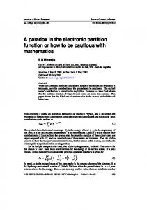
Let Pn denote the set fi =< an ;


; ak ;


a0 >g of all binary partitions of 2n . Several characteristics of Pn are readily apparent. First, an 6= 0 if and only if ak = 0 for all 0  k < n. Second, since the right hand side is even and all terms ak
2k , k > 0 must be even, the coecient a0 must be even. Third, if <


; ak ; ak?1;


> is a partition of Pn , then <


; ak ? 1; ak?1 + 2;


> must be as well. And fourth, if < an ;


; ak ;


; ao > is a partition in Pn then < an ;


; ak ;


; a0; 0 > is a partition in Pn+1 . With these observations, it is not dicult to write a process which generates all partitions in lexicographic order. Doing so, and displaying each partition, generates the following enumerations of P3 and P4 . It is quite easy to verify by inspection that each sequence is a 1 0 0 0 0 0 0 0 0 0

n = 3 0 0 2 0 1 2 1 1 1 0 0 4 0 3 0 2 0 1 0 0

0 0 0 2 4 0 2 4 6 8

1 0 0 0 0 0 0 0 0 0 0 0 0 0 0 0 0 0

0 2 1 1 1 1 1 1 1 1 1 0 0 0 0 0 0 0

0 0 2 1 1 1 0 0 0 0 0 4 3 3 3 2 2 2

0 0 0 2 1 0 4 3 2 1 0 0 2 1 0 4 3 2

n = 4

0 0 0 0 2 4 0 2 4 6 8 0 0 2 4 0 2 4

0 0 0 0 0 0 0 0 0 0 0 0 0 0 0 0 0 0

0 0 0 0 0 0 0 0 0 0 0 0 0 0 0 0 0 0

2 2 1 1 1 1 1 1 1 0 0 0 0 0 0 0 0 0

1 0 6 5 4 3 2 1 0 8 7 6 5 4 3 2 1 0

6 8 0 2 4 6 8 10 12 0 2 4 6 8 10 12 14 16

Figure 1: P3 and P4 partition of 2n . And because they are in lexicographic order, one can verify that all possible 3

partitions have been generated. Because < an?1 ;


; a0 >2 Pn?1 implies < an?1 ;


; a0; 0 >2 Pn , it follows that b(2n ) = b(2n?1) + pn

(6)

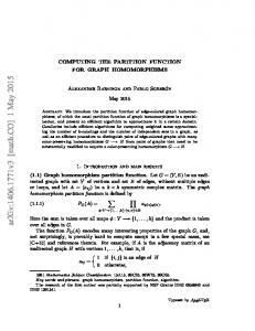
where pn denotes the number of partitions i 2 Pn in which a0 6= 0. We say such partitions are normal because they correspond to closure spaces in which the empty set is closed. In the lexicographic order of Pn , if in =< an ;


; a2; a1; 0 >2 Pn ; a1 6= 0, then there must follow the sequence San1 of partitions, < an ;


; a2; a1 ? 1; 2 >, < an ;


; a2; a1 ? 2; 4 >,


, < an ;


; a2; 0; 2a1 >. There are two such sequences in P3; < 0; 1; 2; 0 > followed by < 0; 1; 1; 2 > and < 0; 1; 0; 4 >, and < 0; 0; 4; 0 > followed by < 0; 0; 3; 2 >; < 0; 0; 2; 4 >; < 0; 0; 1; 6 >; and < 0; 0; 0; 8 >. In P4 there are 6 such subsequences because there are 6 normal partitions in P3 ; the last consists of 8 normal partitions following < 0; 0; 0; 8; 0 >. Once this pattern is perceived the counting process becomes evident. In Figure 2 we reinforce this pattern by showing just the rst 8 and the last 34 (of 202) partitions in P5. 1 0 0 0

0 2 1 1

0 0 0 0 0 0 0 0 0 0 0 0 0 0 0 0 0

0 0 0 0 0 0 0 0 0 0 0 0 0 0 0 0 0

0 0 2 1 . . . 0 0 0 0 0 0 0 0 0 0 0 0 0 0 0 0 0

0 0 0 2

0 0 0 0

0 0 0 0

2 2 1 1 1 1 1 1 1 1 1 1 1 1 1 1 1

1 0 14 13 12 11 10 9 8 7 6 5 4 3 2 1 0

22 24 0 2 4 6 8 10 12 14 16 18 20 22 24 26 28

n = 5

0 0 0 0

1 1 1 1

1 1 1 1

0 0 0 0 0 0 0 0 0 0 0 0 0 0 0 0 0

0 0 0 0 0 0 0 0 0 0 0 0 0 0 0 0 0

0 0 0 0 0 0 0 0 0 0 0 0 0 0 0 0 0

1 1 1 0 . . . 0 0 0 0 0 0 0 0 0 0 0 0 0 0 0 0 0

2 1 0 4

0 2 4 0

16 15 14 13 12 11 10 9 8 7 6 5 4 3 2 1 0

0 2 4 6 8 10 12 14 16 18 20 22 24 26 28 30 32

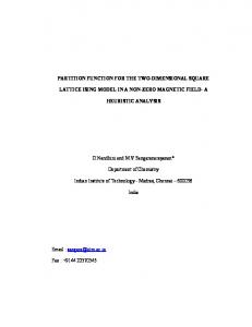
Figure 2: First 8 and last 34 partitions of P5 Notice that these subsequences of normal partitions (with a0 6= 0) were generated by the three normal partitions < 0; 1; 1; 1; 2 >; < 0; 0; 0; 1; 14 >, and < 0; 0; 0; 0; 16 > of P4 . The length of a sequence San1 is a1 . Hence, each normal partition in?1 2 Pn?1 gives rise to a subsequence of an1 = an0 ?1 normal partitions in Pn . If one carefully keeps track of all normal permutations in Pn?1 , then one can use the mechanism above to generate all 4

n =

1

2

3 2

2

)4

=

2 4

6

2

)4

=

)8

=

4 2

)4

=

2 4 6 =) 8 2 =) 4 2 4 6 =) 8 2 4 6 8 10 =)12 2 4 6 8 10 12 14 =)16

5

)2 )2 )2 )2 )2 )2 )2 )2 )2 )2 )2 )2 )2 )2 )2 )2 )2 )2 )2 )2 )2 )2 )2 )2 )2 )2

= = = = = = = = = = = = = = = = = = = = = = = = = =

4 4 4 4 4 4 4 4 4 4 4 4 4 4 4 4 4 4 4 4 4 4 4 4 4 4

6 8 6 8 6 8 10 12 6 8 10 12 14 16 6 8 6 8 6 8 10 12 6 8 10 12 14 16 6 6 6 6 6

8 8 8 8 8

10 10 10 10

12 12 14 16 12 14 16 18 20 12 14 16 18 20 22 24

6 6 6 6 6 6 6

8 8 8 8 8 8 8

10 10 10 10 10 10

12 12 12 12 12 12

14 14 14 14 14

16 16 16 16 16

18 18 18 18

20 20 22 24 20 22 24 26 28 20 22 24 26 28 30 32

Figure 3: a0 coecient in sequences Skn of normal partitions normal partitions in Pn . This is illustrated in Figure 3 in which subsequences Skn of normal partitions are enumerated (by showing only the a0 value) in vertical columns for n = 1 through 4, and horizontally (to conserve space) for n = 5. For n = 1 through 4, each entry an0 in Sin denotes to its right (with )) the last entry < 2a1 ; 0;


; an+1 > in the sequence San0+1 that it generates. Observe in this gure, that when n = 3, all 6 partitions with a0 6= 0 are enumerated in just two subsequences S23 and S43, which were generated by the two normal partitions in P2. With n = 4 the 26 normal partitions of P4 are enumerated in two occurrences of the subsequences S24 and S44, together with single occurrences of S64 and S84, which themselves were generated from the 6 normal partitions of P3 . Fortunately, since all sequences Skn have the form 2, 4,


; k, we need only keep track of the number of such sequences in Pn , not their actual composition. Let kn , k even, denote the number of subsequences Skn of normal partitions in Pn . Based on Figure 3 we can construct Table 1. Since every normal partition of Pn belongs to such a subsequence, we have pn =

X?

2n 1

even k

5

k
kn

(7)

n pn k

2 2

3 4 5 6 6 26 166 1,626 kn

2 1 1 2 6 26 1 2 6 26 4 6 1 4 20 1 4 20 8 10 2 14 2 14 12 14 1 10 1 10 16 18 6 6 20 22 4 4 24 26 2 2 28 30 1 1 32 Table 1: Counts kn of subsequences Skn of normal partitions in Pn Using Table 1 and equation (7) one obtains p7 = 25; 510, and by (6) b(26) = 1; 828, so b(27) = b(26) + p7 = 27; 338. It only remains to determine kn+1 ; 2  k  2n given jn ; 2  j  2n?1 . Since each sequence Skn?1 of normal partitions in Pn?1 generates the subsequences S2n ; S4n;


; S2nk in Pn , one can simply loop over all such subsequences kn?1 and increment 2n ;


2nk as in the following code section max k = 2**(n-1); for (k=2; k