Evaluating the Efficacy of Statistical Simulation for Design Space Exploration Ajay Joshi1, Joshua J. Yi 2, Robert H. Bell Jr.3, Lieven Eeckhout 4, Lizy John1, and David Lilja5 1
- Department of Electrical and Computer Engineering The University of Texas at Austin, Texas {ajoshi,ljohn}@ece.utexas.edu 3
- IBM Systems and Technology Group Austin, Texas
[email protected] 5
2
- Networking and Computing Systems Group Freescale Semiconductor, Inc.
[email protected] 4
- ELIS Department Ghent University, Belgium
[email protected]
- Department of Electrical and Computer Engineering University of Minnesota at Twin Cities
[email protected]
Abstract Recent research has proposed statistical simulation as a technique for fast performance evaluation of superscalar microprocessors. The idea in statistical simulation is to measure a program's key performance characteristics, generate a synthetic trace with these characteristics, and simulate the synthetic trace. Due to the probabilistic nature of statistical simulation the performance estimate quickly converges to a solution, making it an attractive technique to efficiently cull a large microprocessor design space. In this paper, we evaluate the efficacy of statistical simulation in exploring the design space. Specifically, we characterize the following aspects of statistical simulation: (i) fidelity of performance bottlenecks, with respect to cycleaccurate simulation of the program, (ii) ability to track design changes, and (iii) trade-off between accuracy and complexity in statistical simulation models. In our characterization experiments, we use the Plackett & Burman (P&B) design to systematically stress statistical simulation by creating different performance bottlenecks. The key results from this paper are: (1) Synthetic traces stress at least the same 10 most significant processor performance bottlenecks as the original workload, (2) Statistical simulation can effectively track design changes to identify feasible design points in a large design space of aggressive microarchitectures, (3) Our evaluation of 4 statistical simulation models shows that although a very detailed model is needed to achieve a good absolute accuracy in performance estimation, a simple model is sufficient to achieve good relative accuracy, and (4) The P&B design technique can be used to quickly identify areas to focus on to improve the accuracy of the statistical simulation model.
1. Introduction In computer architecture, the simulation of benchmarks is a widely used technique for evaluating computer performance. Computer architects and researchers use
microprocessor models to accurately make performance projections during the pre-silicon phase of the chip design process, and also to quantitatively evaluate microprocessor innovations. Unfortunately, when using a detailed cycleaccurate performance model, the simulation time may span several weeks or months. Further compounding this problem is the growing complexity of microarchitectures (i.e., decreasing simulation speed) and the increasing executiontimes of modern benchmarks. Therefore, in order to meet the time-to-market requirements of a microprocessor, designers use different simulation models during the various stages of the design cycle. Although a detailed and highly accurate cycle-accurate simulator is necessary to evaluate specific design points later in the design cycle, earlier in the design cycle, a simulation technique that has a short development time and can quickly provide performance estimates with reasonable accuracy is desirable. Accordingly, computer architecture researchers have proposed several simulation and modeling techniques that reduce the time needed to generate quantitative performance estimates early in the design cycle. These techniques include analytical modeling of microprocessors [24], statistical modeling of microprocessors [5], hybrid analytical and statistical modeling [12], statistical simulation [15], sampling [22] [25], and reducing the input set of the workload to be simulated [1]. The basic idea in statistical simulation [15] is to model a workload's important performance characteristics with a synthetic trace, and execute the trace in a statistical simulator to obtain a performance estimate. Since the performance estimate quickly converges, the simulation speed of statistical simulation makes it an attractive technique to quickly explore a large design space. Although previous work has shown that statistical simulation has good absolute and relative accuracy and is a viable tool for design space exploration [11] [14] [23], researchers and architects are reluctant to use statistical simulation due to questions such as: (i) What is the absolute and relative accuracy across a diverse set of processor
configurations?, (ii) Does the synthetic trace stress the same bottlenecks as the original program to the same degree?, (iii) Which processor and memory parameters can/cannot be sized using statistical simulation?, (iv) What is the trade-off between simulation accuracy and the complexity of various statistical simulation models?, and (v) Which workload characteristics are inadequately represented in the synthetic trace? The objective of this paper is to answer these questions and systematically analyze the efficacy of statistical simulation as a design space exploration tool. Specifically, we make the following contributions in this paper: 1) We use P&B design-based processor configurations as a stress test for statistical simulation, to evaluate the representativeness of the synthetic trace in terms of its performance bottlenecks. 2) We characterize and examine the ability of statistical simulation to track microprocessor design changes across a diverse set of processor configurations. 3) We compare the level of accuracy and complexity between statistical simulation models that span the range of models that have been proposed. 4) We show how the P&B design technique can quickly and precisely identify areas to focus on to improve the accuracy of the statistical simulation model. The remainder of this paper is organized as follows: Section 2 describes related work, while Section 3 presents a brief overview of statistical simulation and the framework we have used in this study. Section 4 describes the benchmarks used for the evaluation experiments. Section 5 presents the results from our evaluation of statistical simulation. In Section 6 we show how the P&B design can be used to identify areas where one should focus on to improve the statistical simulation model, and Section 7 summarizes the conclusions and key results from our work.
2. Related Work In this section, we discuss prior work on statistical simulation and the characterization techniques that have been used to evaluate simulation methodologies. Oskin et al. [16] proposed a hybrid processor simulator, HLS, which uses statistical and symbolic execution to evaluate design alternatives. They generated a statistical profile from a normal distribution of workload characteristics, and simulated it on a generalized superscalar execution model. Their results showed good correlations with the SimpleScalar and MIPS R10K processor models. Bell et al. [18] improved the correlation of HLS by modeling the workload at the granularity of the basic block and modifying
the generalized microprocessor simulation model to more closely reflect components in a modern superscalar processor. Eeckhout [13] et al. improved the accuracy of performance predictions in statistical simulation by measuring conditional distributions and incorporating memory dependencies using more detailed statistical profiles, and guaranteeing syntactical correctness of synthetic traces. Nussbaum and Smith [23] proposed correlating characteristics such as the instruction type, instruction dependencies, cache behavior, and branch behavior to the size of the basic block. They also compared the accuracy of several models for synthetic trace generation. In [14], Eeckhout et al. showed that the accuracy of statistical simulation can be substantially improved by creating an accurate statistical profile of a workload by using statistical flow graphs to capture the control flow behavior of a program. Eeckhout [11] [14] et al. demonstrated that statistical simulation is capable of efficiently identifying a region of interest in the early stages of the microprocessor design cycle while considering performance and power consumption. Yi et al. [8] proposed to use the P&B design to choose processor parameters, to select a subset of benchmarks, and to analyze the effect of a processor enhancement. Also, Yi et al. [9] used the P&B design as a characterization technique to compare simulation techniques.
3. Statistical Simulation Framework In this paper, we developed an enhanced version of HLS++ [18] statistical simulation framework, called SSHLS++, as our statistical simulation environment. It consists of three steps: 1) Profiling the benchmark program to measure a collection of its execution characteristics to create a statistical profile, 2) Using the statistical profile to generate a synthetic trace, and 3) Simulating the instructions in the synthetic trace on a trace-driven simulator to obtain a performance estimate. Figure 1 illustrates these steps. In the first step, we characterize the benchmark by measuring its microarchitecture-independent and microarchitecture-dependent program characteristics. The former is measured by functional simulation of the program; examples include: instruction mix, basic block size, and the data dependency among instructions. Note that these characteristics are related only to the functional operation of the benchmark’s instructions and are independent of the microarchitecture on which the program executes. On the other hand, the microarchitecture-dependent characteristics include statistics related to the locality and branch behavior of the program. Typically, these statistics include L1 I-cache and D-cache miss-rates, L2 cache miss-rates, instruction and data TLB miss-rates, and branch prediction accuracy. The complete set of microarchitecture-dependent and microarchitecture-independent characteristics form the statistical profile of the benchmark.
Benchmark Binary
Cache and Branch Simulator
Microarchitecture Independent Profiler
Statistical Profile - Instruction Mix - Basic Block Size - Data dependency distance - L1 I-cache miss-rate - L1 D-cache miss-rate - L2 cache miss-rate - D/I TLB miss-rates - Branch Prediction Accuracy
Synthetic Trace Generator
Synthetic Trace
Statistical Simulator
Figure 1. SS-HLS++ statistical simulation framework After generating the statistical profile, the second step is to construct a synthetic trace with similar statistical properties as the original benchmark. The synthetic trace consists of a number of instructions contained in basic blocks that are linked together into a control flow graph, similar to conventional code. However, instead of actual arguments and opcodes, each instruction in the synthetic trace is composed of a set of statistical parameters, such as: instruction type (integer add, floating-point divide, load, etc.), ITLB/L1/L2 Icache hit probability, DTLB/L1/L2 D-cache hit probability (for load and store instructions), probability of branch misprediction (for branch instructions), and dynamic data dependency distance (to determine how far a consumer instruction is away from its producer). The values of the statistical parameters describing each instruction are assigned by using a random number generator following the
distributions of the various workload characteristics in the statistical profile of the benchmark. Finally, in the third step, the synthetic trace is executed on a trace-driven statistical simulator. The statistical simulator is similar to a trace-driven simulator of real program traces, except that the statistical simulator probabilistically models cache misses and branch mispredictions. During simulation, the misprediction probability that is assigned to the branch instruction is used to determine whether the branch is mispredicted, and if so, the pipeline is flushed when the mispredicted branch executes. Likewise, for every load instruction and instruction cache access, the simulator assigns a memory access time depending on whether it probabilistically hits or misses in the L1 and L2 cache. Although, these statistical simulation models that have been recently proposed differ in the complexity of the model used to generate the synthetic trace, fundamentally, each model uses the same general framework described in Figure 1. They primarily differ in the granularity (basic block level, program level, etc.) at which they measure the workload characteristics in the statistical profile. For this study, we implemented the following four statistical simulation models: 1) HLS [16]: This is the simplest model where the workload characteristics (instruction mix, basic block size, cache miss-rates, branch misprediction rate, and dependency distances) are averaged over the entire execution of a program. This model assumes that the workload characteristics are independent of each other and are normally distributed. A synthetic trace of 100 basic blocks is then generated from a normal distribution of these workload statistics and simulated on a general superscalar execution model until the results (Instructions-Per-Cycle) converge. Since the synthetic instructions are few in number and are probabilistically generated, the results converge very quickly. 2) HLS + BBSize: We implemented a slightly modified version of the model proposed in [23]. In this model, other than the basic block size, all workloads characteristics are averaged over the entire execution of the program. However, for the basic block size, we maintain different distributions of the basic block size based on the history of recent branch outcomes. 3) Zeroth Order Control Flow Graph (CFG, k=0) [14] [18]: In this modeling approach, we average the workload characteristics at the basic block granularity (instead of averaging them over the entire execution of the program). While building the statistical profile, we create a control flow graph of the program. This control flow graph stores the dynamic execution frequencies of each unique basic block along with the
transition probabilities to its successor basic blocks. The workload characteristics (instruction mix, cache miss-rates etc.) are measured for each basic block. Since the statistical profile is now at the basic block level, the size of the profile for this model is considerably larger than for the first two. When generating a synthetic trace, we probabilistically navigate the control flow graph and generate synthetic instructions based on the workload characteristics that were measured for each basic block. 4) First Order Control Flow Graph (CFG, k=1) [14]: This is the state-of-the art modeling approach [4]. This approach is the same as the one described in the Zeroth Order Control Flow Graph model described above, except that all workload characteristics are measured for each unique pair of predecessor and successor basic blocks in the control flow graph, instead of just for a unique single basic block. Gathering workload characteristics at this granularity improves the modeling accuracy in the synthetic trace because the performance of a basic block depends on the context (predecessor basic block) in which it was executed. The First Order Control Flow Graph model is the stateof-the-art statistical simulation model, and we therefore use it in all the experiments in this paper. In Section 5.3, we compare the accuracy of the other three models described above against the accuracy of the First Order Control Flow Graph model. Table 1. SPEC CPU 2000 benchmarks and input sets used in this paper
Benchmark 175.vpr-Place 175.vpr-Route 176.gcc 179.art 181.mcf 183.equake 253.perlbmk 255.vortex 256.bzip2
Input Set ref.net ref.arch.in 166.i -startx 110 ref.in ref.in diffmail lendian1 ref.source
Type Integer Floating-Point Integer Floating-Point Integer Floating-Point Integer Integer Integer
4. Benchmarks We used 9 benchmark programs and their reference input sets from the SPEC CPU 2000 benchmark suite in this paper. All benchmark programs were compiled using SimpleScalar’s version of the gcc compiler, version 2.6.3, at optimization level –O3. Table 1 lists the programs, their input sets, and benchmark type. In order to compare the
statistical simulation results for the configurations used in P&B design to the corresponding results from a cycleaccurate simulator, we had to run 44 cycle-accurate simulations of reference input sets for every benchmark program. To reduce this simulation time, we simulated the first one billion instructions only for each benchmark.
5. Evaluating Statistical Simulation In this section we characterize and evaluate the accuracy of statistical simulation. The objective of our characterization is to analyze the efficacy of statistical simulation as a design space exploration tool by stressing it using a number of aggressive configurations. Using aggressive configurations affords us an opportunity to evaluate the accuracy of statistical simulation by systematically exposing a diverse set of processor performance bottlenecks. Our evaluation consists of three parts: In Section 5.1 we evaluate the ability of statistical simulation to identify important processor performance bottlenecks. Specifically, we use a P&B design that uses a number of diverse configurations to evaluate the representativeness of the synthetic trace in terms of its performance bottlenecks. In Section 5.2, we measure the relative accuracy of statistical simulation by examining its ability to accurately track design changes across 44 aggressive processor configurations. Finally, in Section 5.3, we measure the absolute and relative accuracy of the four previously described statistical simulation models, and discuss the trade-offs between their complexity and level of accuracy.
5.1. Identifying Important Processor Bottlenecks Due to their inherent characteristics, different benchmark programs stress different processor performance bottlenecks to different degrees. Since architects use benchmark programs to make quantitative evaluations of various points in the design space and propose processor enhancements to relieve specific performance bottlenecks, the synthetic trace used in statistical simulation should have the same key microprocessor performance bottlenecks that are present when simulating the benchmark on a cycle-accurate simulator. We quantify the representativeness of the synthetic trace by quantifying the difference between the bottlenecks stressed by the original workload and the synthetic trace. For architects, the P&B design [8] can determine which processor and memory parameters have the largest effect on performance (cycles-per-instruction) i.e., identify the biggest performance bottlenecks. The P&B design is a very economical experimental design technique that varies N parameters simultaneously over approximately (N + 1) simulations [20]. Based on the results of the P&B design, we assign a rank for each performance bottleneck based on its P&B magnitude. The P&B magnitude represents the significance of that bottleneck, or more specifically, the effect that the bottleneck has on the variability in the output value,
programs, we analyzed the absolute values of the P&B magnitude. For 179.art and 183.equake, the absolute values of P&B magnitudes for the most important and the least important parameters ranges from 138 (L2 cache size) to 1 (the number of Return Address Stack entries) and 80 (L1 Icache size) to 0.4 (I-TLB associativity), respectively. Note that larger differences in the P&B magnitudes imply larger performance impacts for that bottleneck. Therefore, in benchmarks such as 179.art and 183.equake, the importance of the most and least significant parameter is very distinct. However, for 256.bzip2, the difference in the significance of the bottlenecks is less distinct since the range of magnitudes is only 16. Since the importance of the most and least significant bottlenecks is not substantially different, incorrectly estimating the importance of bottlenecks that have relatively little impact on the CPI does not imply any additional inaccuracy on the part of statistical simulation. Top 3 Bo ttlene cks Top 15 Bottlen ecks
60
Top 5 Bo ttlene cks Top 20 b ottlen ecks
Top 10 bo ttlen ecks Top 41 bo ttlen ecks
50
Norm alizedEuclideanDistance(0-100)
40
30
20
10
Average
256.bzip2
255.vortex
253.perlbm k
183.equake
181.m cf
179.art
176.gcc
175.vpr.Route
0
175.vpr.Place
e.g., cycles-per-instruction (CPI). The bottleneck that has the largest impact on the CPI, i.e., the microarchitectural parameter with the highest P&B magnitude, is the largest performance bottleneck in the processor core and memory subsystem. Based on their significance, we assign a rank to each bottleneck, i.e., the most significant bottleneck has a rank of 1, while the least significant has a rank of N. In this study, we evaluated 43 parameters in an out-oforder superscalar microprocessor related to the L1 I-cache, L1 D-cache, L2 cache, instruction and data TLB, branch predictor configuration, integer execution units, and floating point execution units. To determine the P&B magnitude, and subsequently the rank, of each bottleneck, we use 44 very different processor configurations. The configurations represent the “envelope of the hypercube” of processor configurations and provide a stress test for statistical simulation by systematically exposing diverse performance bottlenecks. To characterize our bottlenecks, the input parameter values were set to low and high values that were similar to those found in [8]. To quantify the representativeness of the synthetic trace, we first vectorize the ranks (from statistical simulation and cycle-accurate simulation) and then compute the Euclidean distance between the pair of vectors. Smaller Euclidean distances indicate that the ranks from statistical simulation are very similar to those obtained by simulating the program with a cycle-accurate simulator. When the vectors of ranks are identical (i.e., the significance of each bottleneck is the same for both statistical and cycle-accurate simulation), the Euclidean distance is 0. When the ranks are completely “out-of-phase” (i.e. versus ), the Euclidean distance is at a maximum of 162.75. We normalize the Euclidean distance between each pair of vectors to this maximum, and then scale the distance to a 0 to 100 range. Since the ranks for all bottlenecks are included in the Euclidean distance, insignificant bottlenecks may deceptively inflate the Euclidean distance. Additionally, one has to be careful when interpreting the results based only on the ranks of the parameters. It is possible that while the Euclidean distance is fairly high, their significance may be, in fact, quite similar. In such cases, seemingly large Euclidean distances are the result of quantization error due to using ranks. To avoid such a pitfall, we also separately present the normalized Euclidean distance for the most significant 3, 5, 10, and 20 parameters, in addition to all 43. Figure 2 shows the normalized Euclidean distance for the 9 benchmarks. The results in this figure show that statistical simulation can identify the 10 most important bottlenecks for all programs with good accuracy (normalized Euclidean distance less than or equal to 15). For all 43 bottlenecks, the accuracy is very high for 179.art, good for 176.gcc and 183.equake, moderate for 175.vpr-Place, 175.vpr-Route, and 253.perlbmk, and poor for 181.mcf, 255.vortex, and 256.bzip2. In order to understand the reasons for the difference in level of accuracy of statistical simulation for different
Figure 2. Normalized Euclidean distance (0 to 100) between the ranks of processor and memory performance bottlenecks estimated by statistical simulation and cycle-accurate simulation. Smaller Euclidean distances imply higher representativeness of synthetic trace. In any case, the primary goal of early design space studies is to identify a range of feasible design values for the most important performance bottlenecks. Since we observe that statistical simulation can do so, we conclude that statistical simulation is useful during early design space exploration. For programs such as 176.gcc, 179.art, and 183.equake, since the synthetic trace is very representative for all 43 bottlenecks stressed by the original benchmark program, statistical simulation may be a valuable tool even beyond the earliest stages of the design space exploration studies.
5.2. Tracking Design Changes During early design space exploration, the ability of a simulation technique, e.g., statistical simulation, to accurately predict a performance trend, is a very important feature. Or, in other words, the relative accuracy of statistical simulation is more important than its absolute accuracy. If a simulation
175.vpr-Place
5.5
A c tual
SS-HLS++
3.5
2.5 2
2
1
1.5
0.5
0
0 5
7
1 0.5
9 11 13 15 17 19 21 23 25 27 29 31 33 35 37 39 41 43
1
3
5
7
179.art
0
9 11 13 15 17 19 21 23 25 27 29 31 33 35 37 39 41 43
Configuration
6
3 2.5
1.5
1 0.5 3
Speedup
4
3 Speedup
Speedup
4.5
3.5
2
1
A ctual
SS-HLS++
5
4.5
4.5
Actual
181.m cf
5.5 5
2.5
3 2.5
2
2
1.5
1.5
1
1
0.5
1.5 1 0.5 0 1
9 11 13 15 17 19 21 23 25 27 29 31 33 35 37 39 41 43
1
3
5
7
Configuration
253.perlbmk
A c tual
3
5
7
9 11 13 15 17 19 21 23 25 27 29 31 33 35 37 39 41 43
9 11 13 15 17 19 21 23 25 27 29 31 33 35 37 39 41 43 Configuration
SS-HLS++
A ctual
255.vorte x
6
6
SS-HLS++
3.5 3 2.5 2
0 7
A ctual
183.e quak e
0.5
0
9 11 13 15 17 19 21 23 25 27 29 31 33 35 37 39 41 43 Configuration
5 4.5 4 Speedup
Speedup
3
5
7
5.5
3.5
3.5
3
5
SS-HLS++
4
4
1
3
Configuration
5.5
SS-HLS++
5
4 3 2.5
Ac tual
176.gcc
5.5
3.5
1
Speedup
SS-HLS++
4
1.5
Configuration
SS-HLS++
A ctual
256.bzip2
4
SS-HLS++
5.5
5.5
3.5
5
5
4.5 4 3.5
Speedup
4 3.5 3 2.5
3 Speedup
4.5 Speedup
Actual
175.vpr-Route
4.5
5 4.5
3 2.5
2
2
1.5
1.5
1
1
0.5
0.5 1
3
5
7
9 11 13 15 17 19 21 23 25 27 29 31 33 35 37 39 41 43 Configuration
2 1.5 1 0.5 0
0
0
2.5
1
3
5
7
1
9 11 13 15 17 19 21 23 25 27 29 31 33 35 37 39 41 43 Configuration
3
5
7
9 11 13 15 17 19 21 23 25 27 29 31 33 35 37 39 41 43 Configuration
Figure 3. Actual and estimated speedup across 43 processor configurations for 9 SPEC CPU2000 benchmarks.
RS = 1 – 6 ∑ di2/ (n3-n)……………………………(i)
where di is the difference between ranks estimated for ith configuration and n is the total number of configurations. The value of RS ranges from -1 to 1. A value of 1 for RS indicates that statistical simulation correctly estimated the ranks for all configurations (highest relative accuracy), and a value of -1 means that the ranks estimated by statistical simulation are perfectly opposite to the ones estimated from cycle-accurate simulation (lowest relative accuracy). 1.00 0.90 0.80 0.70 0.60 0.50 0.40 0.30 0.20 0.10
Average
256.bzip2
255.vortex
253.perlbmk
183.equake
181.mcf
179.art
176.gcc
175.vpr.Route
0.00
175.vpr.Place
Spearman's Rank Correlation (0-1)
technique exhibits good relative accuracy, it means that the technique will accurately track performance changes, and therefore can help to identify the interesting design points that need to be further analyzed using detailed simulation. To evaluate the relative accuracy, we used the 44 P&B configurations that represent a wide range of processor configurations. It is important to note that while these processor configurations are not realistic, they enable us to evaluate whether statistical simulation is accurate enough to track the processor’s performance across a wide range of configurations. The approach that we used to characterize the relative accuracy of statistical simulation was to examine the correlation between the estimated and actual ranking of the configurations. In particular, we measured the speedup in CPI obtained from statistical simulation and cycle-accurate simulation for 43 configurations relative to the 44th configuration, and ranked the 43 processor configurations in descending order of their speedups. Figure 3 shows the individual speedups for each configuration for all benchmark programs. We observe that in general, across all programs, statistical simulation tracks both local and global speedup minima/maxima extremely well. We now use Spearman’s rank correlation coefficient to measure the relation between the ranks estimated by cycleaccurate and statistical simulation. The Spearman’s rank correlation coefficient is calculated as:
Figure 4. Relative Accuracy in terms of Spearman’s correlation coefficient between actual and speedups across 43 processor configurations
estimated
Figure 4 shows that the relative accuracy is very good for all programs (> 0.95). This suggests that for all programs, the
5.3. Comparing the Accuracy of Statistical Simulation Models
absolute error is 11% for the First Order Control Flow Graph (CFG, k=1) statistical simulation model, which is very similar to the level of accuracy in previously published work [4].) HLS
50
HLS+BBSize
CFG(k=0)
CFG(k=1)
88.6%
45 40 % Error in CPI
ranks for the 43 configurations estimated by statistical simulation are very similar to the ranks estimated from cycleaccurate simulation. From these results, we conclude that statistical simulation can be effectively used to narrow down a large design space to a few feasible design points. Subsequently, the architect can use a more accurate simulation technique to further study these feasible design points.
35 30 25 20 15 10 5 Average
256.bzip2
255.vortex
253.perlbm k
183.equ ake
181.mcf
179.art
176.gcc
175.vpr.Route
175.vp r.Place
0
Figure 5. Comparison between absolute accuracy of 4 statistical simulation models on the 44 extreme processor configurations HLS
1.00
HLS+BBSize
CFG (k=0)
CFG(k=1)
0.90 Spearman's Rank Correlation
0.80 0.70 0.60 0.50 0.40 0.30 0.20 0.10 Average
256.bzip2
255.vortex
253.perlbmk
183.equake
181.mcf
179.art
176.gcc
175.vpr.Route
0.00 175.vpr.Place
Researchers have proposed a number of different statistical simulation models that mainly differ in the complexity of the model used to generate the synthetic trace. Fundamentally, each model uses the same general framework described in Figure 1 and is a refinement of the basic approach to statistical simulation. Intuitively, increasing the degree-of-detail in the model should improve the representativeness of the synthetic trace and thus its absolute accuracy. However, what is not clear is how the additional modeling affects the relative accuracy, and whether there is a good trade-off between the model’s complexity and its associated absolute and relative accuracy. In this section, we compare the following 4 modeling approaches, described in Section 3, namely: HLS, HLS+BBSize, Zeroth Order Control Flow Graph (CFG, k=0), and First Order Control Flow Graph (CFG, k=1). We use the 44 P&B configurations to evaluate and compare the absolute error, relative accuracy, and the ability to identify important processor bottlenecks of the four models. The absolute error (AE) is computed as the percentage error in CPI between cycle-accurate simulation (CS) and statistical simulation (SS), that is:
Figure 6. Relative accuracy based on the ability to rank 43 AE = (| CPICS – CPISS|) * 100 / CPICS…………………...(ii) To calculate the relative accuracy, we use the RS measure of relative accuracy as described in equation (i). To measure the fidelity of the processor bottlenecks, we compute the Normalized Euclidean. Distance between the ranks of the bottlenecks from cycle-accurate simulation and statistical simulation for the most significant 5, 20, and all 43 bottlenecks. Figure 5 shows that increasing the level-of-detail in the statistical simulation model improves the absolute accuracy for all benchmarks. For the simplest model, HLS, the AE is 36.8%; for the First Order Control Flow Graph (CFG, k=1), the most sophisticated model, the AE is 16.7%. Therefore, if the primary goal is high absolute accuracy, a computer architect should use as detailed a statistical simulation model as possible to generate the synthetic traces. It is very important to note that the average error of 16.7% for the stateof-the-art statistical simulation model is for the 44 aggressive, unrealistic configurations. (Note that from our experiments with using balanced (realistic) configurations, the average
configurations in order of their speedup
Figure 6 shows the relative accuracy of the 4 simulation models based on the ability of statistical simulation to rank 43 diverse processor configurations in order of their speedups (RS). The figure shows that although there is a large improvement in relative accuracy between the HLS and HLS+BBSize, additional modeling yields only slight improvements in the relative accuracy. Figure 7 shows the results of processor bottleneck characterization for the four statistical simulation models. The accuracy of the HLS model is good enough to identify only top 3 performance bottlenecks for all programs except 181.art and 256.bzip2. By increasing the complexity of the HLS+BBSize model allows statistical simulation to correctly identify the order of the Top 3, 10, 20, and all 43 bottlenecks. The two statistical simulation models, Zeroth Order Control Flow Graph (CFG, k=0) and First Order Control Flow Graph (CFG, k=1), only marginally improves the accuracy to of statistical simulation to identify the performance bottlenecks.
design decisions early in the design cycle when the time and resources for simulator development are very limited.
90 80 70
6. Challenges and Opportunities for Improving Statistical Simulation
60 50 40 30 20 10
HLS
HLS+BBSize
CFG(k=0)
Average
256.bzip2
255.vortex
253.perlbmk
183.equake
181.mcf
179.art
176.gcc
175.vpr.Route
0 175.vpr.Place
Norm. Euclidean Distance (0-100)
100
CFG(k=1)
(a) Top 5 bottlenecks HLS
Norm. Euclidean Distance (0-100)
100
HLS+BBSize
CFG(k=0)
CFG(k=1)
90 80 70 60 50 40 30 20 10 Average
256.bzip2
255.vortex
253.perlbmk
183.equake
181.mcf
179.art
176.gcc
175.vpr.Route
175.vpr.Place
0
(b) Top 20 bottlenecks HLS
Norm. Euclidean Distance (0-100)
100
HLS+BBSize
CFG(k=0)
CFG(k=1)
90 80 70 60 50 40 30 20 10 Average
256.bzip2
255.vortex
253.perlbmk
183.equake
181.mcf
179.art
176.gcc
175.vpr.Route
175.vpr.Place
0
(c) Top 43 bottlenecks Figure 7. Bottleneck characterization for 4 statistical simulation models.
In summary, from these results, we conclude that if absolute accuracy is the primary goal, then the computer architect should use the most detailed state-of-the art statistical simulation model, Control Flow Graph (k=1). However, we observe that an increase in the absolute accuracy of statistical simulation does not result in a commensurate increase in its relative accuracy. Interestingly, a simple statistical model such as HLS+BBSize has the ability to yield very good relative accuracy, although the absolute accuracy is lower. Therefore, one key result from this paper is that simple statistical simulations models have a good relative accuracy, which makes them an effective tool to make
If the synthetic trace models all of the key workload characteristics that affect a benchmark’s performance, the ranks of the bottlenecks from statistical simulation should be very similar to those found using cycle-accurate simulation, such that the Euclidean distance is close to 0. Therefore, by analyzing how well the statistical simulation technique identifies the processor bottlenecks, one can determine which bottlenecks are well represented in the synthetic trace and also identify which bottlenecks need additional modeling effort. In order to determine the overall importance of a bottleneck across all benchmarks, we first find the sum of the rank of each individual parameter for all the benchmark programs. The parameter with the smallest sum of ranks is, on average, the most significant bottleneck that affects performance across all programs. By using this method, we can rank each parameter based on its average significance across all the benchmarks. For each bottleneck, we calculate the difference between its ranks obtained from cycle-accurate simulation and statistical simulation. The maximum difference is 42, so we normalize the distance to obtain a normalized difference between ranks, and then scale it between 0 and 100. Table 2 shows the rank of each bottleneck across the 9 benchmark programs, and the normalized difference between ranks shows how well that bottleneck is modeled in the synthetic trace. The table has been sorted in the ascending order of the parameters that are well represented in the synthetic trace i.e., the number of FP ALUs is the most wellmodeled parameter and I-TLB size is the least. From Table 2, we conclude that the synthetic trace does not model the effect of the following microarchitectural parameters accurately: the I-TLB size, the L1 D-Cache size, the latency of integer multiply execution units, the L2 Cache Block Size, and the number of BTB entries. It is interesting that out of the top 10 least well-modeled bottlenecks, 8 are related to the data locality and control flow predictability of the program. This suggests that in order to improve the representativeness of the synthetic trace, and thus the accuracy of statistical simulation, researchers must expend effort to improve the modeling of data locality and control flow predictability in the synthetic trace. The key advantage of using the P&B design to analyze the strengths and weaknesses of statistical simulation is that it separates the program characteristics that are not modeled very accurately, but which have a large impact on performance (such as branch predictor type, number of LSQ entries, etc.) from the parameters that are also not accurately modeled, but have very little performance impact. This allows us to efficiently allocate our efforts to only improve
modeling deficiencies that actually make a significant impact on the accuracy of statistical simulation. Table 2.
Significance (Rank) of a processor bottleneck (Parameter) and how well (Normalized difference between ranks) the bottleneck is modeled in the synthetic trace. A smaller distance indicates that the parameter is well modeled.
RANK 37 20 26 27 39 41 22 29 9 12 10 16 34 36 42 4 6 13 17 25 8 10 14 19 30 38 4 7 40 3 2 30 1 15 21 22 24 28 33 35 43
PARAMETER I-TLB Size L1 D-Cache Size Int Multiply Latency L2 Cache Block Size BTB Entries Number of Integer Mult/Div Units I-TLB Page Size L1 D-Cache Block Size LSQ Entries BTB Associativity Branch Predictor Type Memory Ports FP Square Root Latency FP Divide Latency Instruction Fetch Queue Entries Int Divide Latency Number of RUU Entries Branch Misprediction Penalty I-TLB Latency I-TLB Associativity FP ALU Latencies Memory Latency First Memory Bandwidth Int ALUs L2 Cache Associativity Number of FP Mult/Div L1 I-Cache Latency L1 I-Cache Block Size L1 I-Cache Associativity L1 I-Cache Size L2 Cache Latency L1 D-Cache Associativity L2 Cache Size FP Multiply Latency D-TLB Associativity D-TLB Size Speculative Branch Update Integer ALU Latencies Return Address Stack Entries L1 D-Cache Latency Number of FP ALUs
NORMALIZED DIFFERENCE BETWEEN RANKS (0-100) 44.2 39.5 30.2 30.2 27.9 25.6 23.3 20.9 18.6 18.6 14.0 14.0 14.0 14.0 14.0 11.6 11.6 11.6 11.6 11.6 9.3 9.3 9.3 9.3 9.3 9.3 7.0 7.0 7.0 4.7 2.3 2.3 2.3 0.0 0.0 0.0 0.0 0.0 0.0 0.0 0.0
7. Conclusions Since detailed cycle-accurate simulation models require long simulation times, computer architects have proposed statistical simulation as a time-efficient alternative for performing early design space exploration studies. But the concern for many architects is that statistical simulation may not perform well for processor configurations that are drastically different than the ones that have been used in previous evaluations, i.e., it is suited only for evaluating incremental changes in processor architectures. The objective of this paper was to evaluate the efficacy of statistical simulation as a design space exploration tool, in wake of these issues and concerns to using statistical simulation. In this paper, we use the Plackett & Burman (P&B) design to measure the representativeness of the synthetic trace. The configurations used in P&B design provide a systematic way to evaluate the accuracy of statistical simulation by exposing various performance bottlenecks. The key results from this paper are: 1) At the very least, synthetic traces stress the same 10 most significant processor performance bottlenecks as the original workload. Since the primary goal of early design space studies is to identify the most significant performance bottlenecks, we conclude that statistical simulation is indeed a very useful tool. 2) Statistical simulation has good relative accuracy and can effectively track design changes to identify feasible design points in a large design space of aggressive microarchitectures. 3) Our evaluation of four statistical simulation models shows that although a very detailed model is needed to achieve a good absolute accuracy in performance estimation, a simple model is sufficient to achieve good relative accuracy. This is very attractive early in the design cycle when time and resources for developing the simulation infrastructure are limited. 4) Computer architects can use the P&B design to quickly identify areas to focus on to improve the accuracy of the statistical simulation model. We applied this technique to the state-of-the-art statistical simulation model and observed that dataflow and control flow predictability must be modeled more accurately in the synthetic trace to further improve the accuracy of statistical simulation. From these results, we conclude that statistical simulation, with its ability to identify key performance bottlenecks and accurately track performance trends using a simple statistical simulation model, is a valuable tool for making early microprocessor design decisions. In addition,
we feel that the methodology used in this paper also provides a framework for researchers to further evaluate and improve the accuracy of statistical simulation.
8. Acknowledgements This research is supported in part by NSF grant 0429806, the IBM Systems and Technology Division, IBM CAS Program, Intel, the University of Minnesota Digital Technology Center, and the University of Minnesota Supercomputing Institute. Lieven Eeckhout is a Postdoctoral Fellow of the Fund for Scientific Research – Flanders (Belgium) (F.W.O Vlaanderen) and is also supported by Ghent University, IWT, the HiPEAC Network of Excellence, and the European SCALA project No. 27648.
9. References [1]
A. KleinOsowski and D. Lilja. MinneSPEC: A New SPEC Benchmark Workload for Simulation-Based Computer Architecture Research. Computer Architecture Letters, vol. 1, June 2002. [2] B. Kumar and E. Davidson. Computer system design using a hierarchical approach to performance evaluation. Communications of ACM, vol. 23, pp. 511-521, Sept. 1980. [3] D. Burger and T. Austin. The SimpleScalar Toolset, version 2.0. University of Wisconsin-Madison Computer Sciences Department Technical Report #1342, 1997. [4] D. Lilja. Measuring Computer Performance. Cambridge University Press, 2000. [5] D. Noonburg and J. Shen. A framework for statistical modeling of superscalar processor Performance. International Symposium on High-Performance Computer Architecture, February 1997. [6] J. Henning. SPEC CPU2000: Measuring CPU Performance in the New Millenium. IEEE Computer, vol. 33 no. 7, pp. 28-35, July 2000. [7] J. Yi and D. Lilja. Effects of Processor Parameter Selection on Simulation Results. MSI Report 2002/146, 2002. [8] J. Yi, D. Lilja, and D. Hawkins. A Statistically Rigorous Approach for Improving Simulation Methodology. International Symposium on High Performance Computer Architecture, 2003. [9] J. Yi, S. Kodakara, R. Sendag, D. Lilja, and D. Hawkins. Characterizing and Comparing Prevailing Simulation Techniques. International Symposium on High Performance Computer Architecture, 2005. [10] K. Skadron, P. Ahuja, M. Martonosi, and D. Clark. Branch Prediction, Instruction-Window Size, and Cache Size: Performance Trade-Offs and Simulation Techniques. IEEE Transactions on Computers, vol. 48, no. 11, pp. 1260-1281, November 1999.
[11] L. Eeckhout and K. De Bosschere. Early Design Phase Power/Performance Modeling through Statistical Simulation. International Symposium on Performance Analysis of Systems and Software. November 2001. [12] L. Eeckhout and K. De Bosschere. Hybrid AnalyticalStatistical Modeling for Efficiently Exploring Architecture and Workload Design Spaces. International Conference on Parallel Architectures and Compilation Techniques. 2001 [13] L. Eeckhout, K. De Bosschere, and H. Neefs. Performance Analysis through Synthetic Trace Generation. International Symposium on Performance Analysis of Systems and Software. April 2000. [14] L. Eeckhout, R. Bell Jr., B. Stougie, K. De Bosschere, and L. John. Improved Control Flow in Statistical Simulation for Accurate and Efficient Processor Design Studies. International Symposium on Computer Architecture, June 2004 [15] L. Eeckhout, S. Naussbaum, J.E. Smith, and K.De Bosschere. Statistical Simulation: Adding Efficiency to the Computer Designer’s Toolbox. IEEE Micro, vol. 23 no.5, pp. 26-38, Sept/Oct 2003 [16] M. Oskin, F. Chong, M. Farrens. HLS: Combining Statistical and Symbolic Simulation to Guide Microprocessor Design. International Symposium on Computer Architecture, pp. 7182, June 2000 [17] R. Bell, Jr. and L. John. Improved Automatic Testcase Synthesis for Performance Model Validation. International Conference on Supercomputing (ICS ’05), June 2005. [18] R. Bell, Jr., L. Eeckhout, L. John and Koen De Bosschere. Deconstructing and Improving Statistical Simulation in HLS, Workshop on Duplicating, Deconstructing and Debunking, in conjunction with ISCA ’04, June 2004. [19] R. Carl and J.E. Smith. Modeling Superscalar Processor via Statistical Simulation. Workshop on Performance Analysis and Its Impact on Design. June 1998 [20] R. Plackett and J. Burman. The Design of Optimum Multifactorial Experiments. Biometrika, vol. 33 no. 4, pp. 305-325, June 1946 [21] R. Savedra-Barrera, A.J. Smith, E. Miya. Machine characterization based on an abstract high-level machine language. IEEE Transactions on Computers, vol. 38, pp. 1659-1679, Dec. 1989. [22] R. Wunderlich, T. Wenish, B. Falsafi, and J. Hoe. SMARTS: Accelerating microarchitecture simulation via rigorous statistical sampling. International Symposium on Computer Architecture, June 2003. [23] S. Nussbaum and J.E. Smith. Modeling Superscalar Processors via Statistical Simulation. International Conference on Parallel Architectures and Compilation Techniques, pp 1524, Sept 2001 [24] T. Karkhanis and J.E.Smith. A First-Order Superscalar Processor Model. International Symposium on Computer Architecture. June 2004. [25] T. Sherwood, E. Perelman, G. Hamerly, and B. Calder. Automatically characterizing large scale program behavior. ASPLOS-X, pp. 45-57, Oct 2002.