Evaluating The Impact of Context-Sensitivity on Andersen’s Algorithm for Java Programs Donglin Liang University of Minnesota Minneapolis, MN 55455, USA
[email protected]
1.
Maikel Pennings and Mary Jean Harrold Georgia Institute of Technology Atlanta, GA 30332, USA {pennings,harrold}@cc.gatech.edu
INTRODUCTION
Program analysis and program optimization of Java programs require reference information that estimates the instances of classes that may be accessed through dereferences. Recent work has presented several approaches for adapting Andersen’s algorithm [1]—the most precise flow-insensitive and context-insensitive points-to analysis algorithm developed for C— for analyzing Java programs (e.g., [5, 9, 12]). Studies in our previous work [6] indicate that this algorithm may compute very imprecise reference information for Java programs. Many reasons account for the imprecision of Andersen’s algorithm. Our previous studies [6] indicate that one important source of imprecision in Andersen’s algorithm is its naming scheme, which uses an allocation site to identify the instances created at this site. In this case, if the instances created at the same allocation site are used by the program in different ways, then the reference information provided by Andersen’s algorithm can be imprecise. Another important source of imprecision in Andersen’s algorithm may be its context-insensitive nature: it computes the same information for the local variables (including formal parameters) in the method, regardless of the context in which the method is invoked. If a local variable in the method can hold different values under different contexts, then the algorithm will compute imprecise information. Existing research has investigated the possibility of improving the precision of Andersen’s algorithm by considering the invocation contexts when analyzing a method. In our previous work [6], we evaluated the context-sensitive naming schemes that introduce different names to identify instances allocated at an allocation site under different invocation contexts. The studies show that such naming schemes may allow a static reference analysis to compute more precise information. Milanova, Rountev, and Ryder [7] adapted Andersen’s algorithm to analyze a method under the context of each specific receiver instance on which the method Permission to make digital or hard copies of all or part of this work for personal or classroom use is granted without fee provided that copies are not made or distributed for profit or commercial advantage and that copies bear this notice and the full citation on the first page. To copy otherwise, to republish, to post on servers or to redistribute to lists, requires prior specific permission and/or a fee. PASTE’05, September 5–6, 2005, Lisbon, Portugal. Copyright 2005 ACM 1-59593-239-9/05/0009 ...$5.00.
is invoked (object-sensitivity). Their studies show that the information provided using this approach may significantly improve the precision of modification side-effect analysis and virtual-method resolution. Despite of these existing works, the effectiveness of using contexts to improve the precision of Andersen’s algorithm is not fully justified and understood. First, how well can context-sensitive naming schemes improve the precision of a static reference analysis? Second, how does objectsensitivity compare to traditional calling-context sensitivity, in which the context for a method invocation is identified using a call-string [11] that consists of the top-most k (k is an integer) callsites that are on the stack when the method is invoked? Third, how would increasing the capabilities of distinguishing contexts for a method affect the precision of the context-sensitive version of Andersen’s algorithm? Answers to the above questions will provide useful insights into the effects of various considerations in designing context-sensitive reference analysis algorithms. Such insights can guide us in developing practical algorithms that achieve the best tradeoff between precision and efficiency. This paper presents a set of empirical studies that seek answers to these questions. We implemented several contextsensitive versions of Andersen’s algorithm using both the calling-context and an extended version of the object-context. We also implemented a profiler that records information for instances that are allocated during program execution. We then compared, on a set of subject programs, the information computed by each version of Andersen’s algorithm with that recorded by the profiler. The studies show a number of interesting results: • Considering contexts improves the precision of Andersen’s algorithm on Java programs in some cases, but not in other cases. • Context-sensitive naming schemes are critical for a context-sensitive version of Andersen’s algorithm to compute more precise information. • Calling-context-sensitivity and object-context-sensitivity complement each other: in some cases, calling-contextsensitivity outperforms object-context-sensitivity; in some other cases, the opposite occurs. The results indicate that a practical context-sensitive version of Andersen’s algorithm may have to use the characteristics of the programs to determine the kind of contexts and the amount of context information when it analyzes different programs or different parts of the same program.
1 class A { 2 Object f; 3 Object get() { 4 return new Object(); 5 } 6 A() { 7 this.f = this.get(); 8 } 9 static main() { 10 A a1 = new A(); 11 A a2 = new A(); 12 Object p = a2.get(); 13 p.toString(); 14 } 15 }
A:this
a1
A:this 10
get:this
a2
A:this 11
a2
get:this 11
get:this10 get:ret o10
o11
f
p
get:ret10
o10
o4 A:this 10
a1
A:this 11
a2
o10 f
o11
o11#4
p
(d) The graph for 1−level context−bounded version A:this 10
get:this
get:this10 get:ret10
f o10#4
(b) The graph for the context−insensitive version 11
get:ret 11
f
a1
A:this 11
a2
get:this7 get:ret7
o10
o11
p
get:this12
get:ret12
f
f
(c) The graph for 1−level name−bounded version
get:ret11
p
o11
f
f
o4
(a) An example program
a1
o7#4
o12#4
(e) The graph for 1−level call−string version
Figure 1: A program and its points-to graphs computed with different versions of Andersen’s algorithm.
2.
THE ANDERSEN’S ALGORITHM
Andersen’s algorithm can be used to compute a points-to graph for a java program. In such a graph, a node represents a variable or an instance, and an edge represents a variable reference (without label) or an instance field reference (labeled with the field name). The algorithm identifies an instance using the allocation site that creates the instance. Figure 1(b) shows the points-to graph constructed by this algorithm for the program in Figure 1(a). Note that, in the graph, a special local variable “ret” is introduced to represent the returned value of method “get()”. We extend Andersen’s algorithm to analyze the methods under each specific context. When a method m is analyzed under a context con, each local variable l in the method is replaced with lcon . If an allocation site in m has a statement number n, then the algorithm uses a name con#n to identify the instances allocated at the allocation site under this context. In this way, the algorithm can compute contextsensitive information. Similar approach has been used in some existing work (e.g., [1, 7]). We consider two kinds of contexts. These contexts will be created during the progress of the algorithm. For efficiency, the size of each context is bounded by a pre-defined constant value so that the algorithm will not create too many contexts. The first kind of context is the call-string context. A k-level call-string context for a method is identified using a string of statement numbers n1 , n2 , ..., nk that identify the top-most k method calls on the stack when the method is invoked, where k is a predefined constant number.1 The second kind of context is the receiver context. A receiver context is derived from the name that identifies the receiver instance on which the method is invoked. In this scheme, a receiver context or the name for an instance is represented as a string of statement numbers n1 , n2 , ..., ni , each of which identifies an allocation site. This string is denoted as n1 #n2 #...#ni . In general, the receiver contexts and the names for instances can be constructed in the following way: a name that identifies the receiver instances 1 In this paper, we assume the statement number for a statement is unique in a program.
of a method can be used as a receiver context for analyzing the method; a string that represents a receiver context will be extended with the statement number of an allocation site to identify the instances allocated at this site under this particular context. There are two approaches for bounding the length of the receiver contexts to a pre-defined constant value k. The first approach (the name-bounded approach) bounds the length of the instance names to k and directly uses these names as receiver contexts. In this approach, when an allocation site with statement number x is being analyzed under the receiver context of n1 #n2 #...#ni , if i < k, then the name for identifying the instances allocated at x under this context would be n1 #n2 #...#ni #x; however, if i >= k, then the name will be ni−k+2 #...#ni #x. Thus, the length of the new name will not exceed k. This approach has been used in Reference [7], in which k can be 1 or 2. The second approach (the context-bounded approach) bounds the length of receiver contexts at each method call. In this approach, if n1 #n2 #...#nj is the name for the receiver instance at method call c and j > k, then nj−k+1 #...#nj will be used to identify the receiver context at c. Given the same bound k, the length of a receiver context for both approaches will not exceed k. However, the context-bounded approach can allow longer strings (up to k + 1 statement numbers) for instance names. Therefore, this approach can better distinguish the instances used by the program than the namebounded approach. Figures 1(c), 1(d), and 1(e) show the points-to graphs constructed for the program in Figure 1(a) using one-level name-bounded receiver contexts, one-level context-bounded receiver contexts, and one-level call-string contexts, respectively. In the graphs, each local variable in a method other than “main” is annotated with a number that represents the context under which the method is being analyzed. By comparing these graphs with the one in Figure 1(b), we can see that considering contexts allows Andersen’s algorithm to compute more precise information for some reference variables. We can also see that, using the one-level contextbounded receiver contexts allows the algorithm to compute
more precise information than using the one-level namebounded receiver contexts, although the two approaches use the same number of contexts at the method calls. We can further see that using context-bounded receiver contexts allows the algorithm to compute more precise information for field “f” of instance “o10” and “o11”, but less precise information for “p”, than using call-string contexts.
3.
THE SETTINGS
We implemented the algorithms discussed in Section 2. Our implementations of the algorithms do not analyze into calls to methods of collections and maps. Instead, they use models to simulate the effects of these calls on the points-to graph. This treatment is justified as the following. First, the details of classes provided by standard library are typically out of the conerns for many software engineering tasks (e.g., program understanding, debugging). Therefore, it would be more effective to pre-analyze these classes and use the summary information for these classes when analyzing the application classes. This approach can significantly cut the analysis cost when analyzing an application that uses a large number of library classes. Second, methods of library classes (e.g., Vector) often have well-defined interaction patterns with the application classes. Therefore, it is possible to effectively summarize the impacts that these methods would have on the application classes. How to perform such summarization automatically in general is out of the scope of this paper. Our implementation also carefully handles reflection using user-provided information. In our studies, we considered eight versions of Andersen’s algorithm: the context-insensitive version (CI), the context-sensitive versions with levels 1-3 call-string contexts (CS1,CS2,CS3), the context sensitive versions with levels 1, 2 name-bounded receiver contexts (NB1,NB2) and levels 1, 2 context-bounded receiver contexts (CB1,CB2). We do not consider algorithms that use higher-level contexts because, for some of the subjects, such algorithms require too much memory. The points-to information computed by different versions of the algorithm are not directly comparable because the algorithms represent the information in different ways. In our studies, we compared the information computed by each algorithm with the dynamic information collected during the program execution to measure the precision of the points-to information. We implemented a profiler using JVMPI2 to collect dynamic information. During the execution of a subject program, when an instance is being created, our profiler records the necessary information to map the instance to the static name that identifies this instance in a static reference analysis. For each instance i, our profiler also records the set of virtual method calls, C[i], at which the instance is used as the receiver. Let N be the name that identifies i in a static reference analysis. The static reference analysis computes a set of method calls, C[N ], that estimates the set of method calls at which the instances identified by N may be receivers during some execution. If the static reference analysis is precise, then C[N ] and C[i] will be the same. However, because the static reference analysis cannot always provide precise information, C[N ] may contain more virtual method calls than C[i]. Thus, the difference between C[i] and C[N ] can be used as a metric for compar2
http://java.sun.com/products/jdk/1.2/docs/guide/jvmpi/.
Subject Size program Locs† Cls Meth antlr 32030 148 1858 jar 1839 8 89 jas 4620 116 413 java cup 10155 35 372 jb 6025 45 548 jess 19317 207 1132 jfe 31636 310 1837 jlex 7351 20 134 jtar 11904 40 202 raja 6369 65 391 sablecc 44521 295 2025 toba 6417 26 196 †Locs are obtained with ommand
Method Coverage And Dyn % 950 682 72% 36 24 67% 295 264 89% 269 206 77% 184 100 54% 974 757 78% 830 726 87% 105 92 88% 147 97 66% 37 32 86% 1598 1376 86% 150 105 70% “wc -l” on the files.
Table 1: Information of the subjects. ing the precision of the information computed by different static reference analyses. This approach is used in previous work [6]. We performed the studies on a set of real Java programs that we collected from various sources. For each subject program, we created, according to the description of the program, a set of test cases to run the programs for collecting dynamic information. These test cases are designed to cover as much code as possible. Table 1 shows the subject programs; many of them have also been used in other studies (e.g., [5, 6, 7]). For each subject program, the table shows the numbers of lines of code (Locs), classes (Cls), methods (M eth), methods analyzed by Andersen’s algorithm (And), and methods executed by at least one of the test cases (Dyn). Note that the size and coverage information shown in the table exclude the library classes. The table also shows the value of Dyn/And as a percentage (%). We use this value to estimate the percentage of executable methods that are covered by our test cases. The table shows that, for many subject programs, our test cases cover more than 70% of the methods that have been analyzed by Andersen’s algorithm. Note that, because some subjects (e.g., jb, jar) contain classes that are analyzed by Andersen’s algorithm but implement various features that are not used in any execution of the program, our test cases cannot achieve a high coverage for such subjects. One major threat that limits our ability to generalize the results concerns the completeness of our test suite. Although we have created test cases to exercise various functionalities of each subject, these test cases are by no means exhaustive. The results may change when different test cases are used. Nevertheless, the results that we obtained offer significant insights into the performance of the context-sensitive versions of Andersen’s algorithm. These insights can guide us to develop better reference analysis algorithms.
4. THE STUDIES This section presents the studies that we performed.
4.1 Study 1: Precision Per Instance The goal of this study is to evaluate the precision of the information provided by different versions of Andersen’s algorithm. Let i be an instance created during the program execution and n be the name that identifies i by a specific algorithm A. Let C[i] be the set of callsites at which the
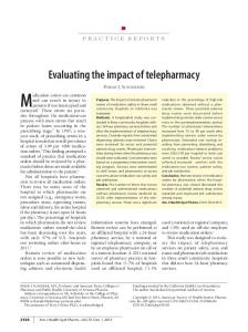
Figure 2: The distribution of the PRVs for instances. Data for jess are not available for higher level contexts because the algorithms ran out of memory. profiler reports i as the receiver, and CA [n] be the set of callsites at which A reports that instances identified by n may be used as the receiver. We compute a precision reference value (PRV) for i, rA [i] by comparing C[i] and CA [n]: rA [i] =
|C[i]| |CA [n] ∩ Cover|
(1)
where Cover the set of callsites that have been exercised by at least one test case. rA [i] indicates the precision of the static reference information with respect to i. If rA [i] = 1, then the static reference information precisely identifies the callsites at which i can be the receiver. However, if rA [i] is much less than 1, then the static reference information identifies many callsites at which i can not be the receiver. Therefore, a programmer or a client analysis that uses such static information may draw inaccurate conclusion about the behavior of the program. Figure 2 shows the results of the study. In the figure, each graph represents the results for one subject program. In each graph, the X-axis shows the algorithms, and the Yaxis shows the percentage of instances whose PRVs are below a certain value. We show the data for each algorithm in a graph using 11 markers. From the bottom up, the first ten markers represent the percentage of instances whose PRVs are less than 0.1, 0.2, 0.3, 0.4, 0.5, 0.6, 0.7, 0.8, 0.9, and 1.0, respectively. The eleventh marker represents the percentage of instances whose PRVs are less than or equal to 1.0. The difference between the 10th marker and the 11th marker represents the percentage of instances whose PRVs are exactly 1.0. Because the PRV for an instance cannot exceed 1.0, the eleventh marker always represents 100%. We use a line to connect the markers that have the same meaning in a graph.
For jar, jas, java cup, jlex, jtar, raja, and toba, all the algorithms compute almost identical information. For these subjects, considering contexts does not seem to improve the precision of Andersen’s algorithm. Thus, we do not show their results in the figure. The graphs show that, for the five subjects, the contextsensitive version of Andersen’s algorithm can compute significantly more precise information for the instances than the context-insensitive version of Andersen’s algorithm. For example, for sablecc, use the information provided by CI, almost 20% of the instances have a PRV less than 0.2 (see the third marker from bottom up); in contrast, using the information provided by CB2, less than 5% of the instances have a PRV less than 0.2. The graphs also show that using higher-level contexts may further improve the precision of the information computed for the instances in some cases, but may have little effect on the precision of the information in other cases. The graphs further show that klevel context-bounded receiver-context-sensitive algorithm can compute more precise information than its k-level namebounded counterpart for some subjects. Since these two versions of Andersen’s algorithm analyze each method under roughly the same number of contexts, they have similar running time for the same subject. Therefore, k-level contextbounded algorithm is preferable over the name-bounded algorithm. By comparing CB1 and CB2 with CS1, CS2, and CS3 on the subjects, we can see that, in real programs, it is possible for the receiver contexts to outperform the callstring contexts; and it is also possible for the call-string contexts to outperform the receiver contexts. In Study 3, we will compare the effectiveness of using different contexts to improve information for instances allocated at each indi-
program antlr(254)
jb(46)
jess(386)
jfe(284)
sablecc(504)
Diff CS3/CI CB2/CI CS3/CB2 CB2/CS3 CS3/CI CB2/CI CS3/CB2 CB2/CS3 CS1/CI CB1/CI CS1/CB1 CB1/CS1 CS3/CI CB2/CI CS3/CB2 CB2/CS3 CS3/CI CB2/CI CS3/CB2 CB2/CS3
(0, 1.0) 19 26 8 18 21 21 10 7 33 41 19 25 80 87 28 49 103 213 12 162
(0, 0.1) 5 14 – 14 2 7 5 7 25 22 16 13 22 38 9 27 10 77 5 109
[0.1, 0.2) 5 6 3 3 11 10 3 – 3 12 3 8 8 10 5 7 7 13 3 16
[0.2, 0.3) 1 2 1 1 5 3 – – 1 4 – 4 3 6 – 6 14 19 2 9
[0.3, 0.4) 3 2 1 – 1 – 1 – – – – – 7 7 1 6 19 25 1 4
[0.4, 0.5) 1 1 1 – – – – – 1 1 – – 13 8 3 1 19 24 1 2
[0.5, 0.6) 1 – 1 – – – – – 1 1 – – 6 4 1 – 18 25 – 8
[0.6, 0.7) 1 – – – – – – – 1 – – – 9 5 2 1 5 10 – 5
[0.7, 0.8) – – – – 1 – 1 – 1 1 – – 7 5 4 1 9 13 – 3
[0.8, 0.9) 2 1 1 – – – – – – – – – 4 1 3 – 1 6 – 5
[0.9, 1.0) – – – – 1 1 – – – – – – 1 3 – – 1 1 – 1
Table 2: The distribution of Dif fA/B [] computed for the allocation sites. vidual allocation site.
4.2 Study 2: Importance of Context-Sensitive Naming Scheme The goal of this study is to evaluate the impact of using context-sensitive naming schemes on the precision of Andersen’s algorithm. Using a context-sensitive naming scheme may allow the algorithm to compute more precise reference information. However, it will also increase the size of the points-to graph, and thus, increase the cost for constructing this graph. For example, without using context-sensitive naming scheme, the Andersen’s algorithm with level-two call-string contexts uses about 600MB memory and terminates in 47 minutes for jess, whereas using the contextsensitive naming scheme, the algorithm uses more than 3.5GB memory and cannot terminate in 10 hours. Thus, the use of such naming scheme needs to be justified. In this study, we evaluate the precision of the contextsensitive Andersen’s algorithms that use a context-insensitive naming scheme: they identify the instances using only the allocation sites. All versions of call-string-context-sensitive algorithms can be modified to use this naming scheme. We refer to these modified versions as SemiCS algorithms. However, because the receiver contexts are computed using information from the instance names, the receiver-contextsensitive algorithms other than NB1 cannot use this naming scheme. Figure 2 has compared NB1 with other versions of Andersen’s algorithm. From the Figure, we can see, for jfe and sablecc, NB1 computes significantly less precise information than CB1. For these subjects, NB1 computes almost the same information as CI. Thus, using the contextinsensitive naming scheme can reduce the effectiveness of improving the precision of Andersen’s algorithm by using receiver contexts. Figure 2 has also compared SemiCS3 (level3 call-context-sensitive with the context-insensitive naming scheme) with other versions of Andersen’s algorithm. The Figure shows that SemiCS3 computes information that is
very close in precision to CI, and that can be significantly less precise than CS3—the corresponding algorithm that use context-sensitive naming scheme. From the above discussion, we can see that the context-sensitive naming schemes are critical to enable a context-sensitive version of Andersen’s algorithm to compute more precise information.
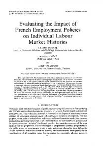
4.3 Study 3: Precision Per Allocation Site The goal of this study is to investigate the impact of considering contexts in Andersen’s algorithm on the precision of the information computed for instances allocated at specific allocation sites. For each allocation site, we compute the average of the PRVs for the instances allocated at this site using the information provided by a specific algorithm A. Let Ia be the set of instances allocated at an allocation site a. We compute the average of the PRVs for the instances in Ia with respect to A using the following formula: P i∈Ia rA [i] r¯A [a] = (2) |Ia | where rA [i] is defined by equation (1). Given algorithms A and B, we compare these two algorithms by computing Dif fA/B [a] = r¯A [a] − r¯B [a] for each allocation site a. Table 2 shows the distribution of the Dif fA/B [] computed for the allocation sites in each subject for a pair of algorithms A and B. In the table, each row represents the results of the comparison between the two algorithms specified as A/B at the second column of the row. The third column in a row represents th total number of allocation sites whose Dif fA/B [] are greater than 0. Starting from the fourth column, each column in a row represents the number of allocation sites whose Dif fA/B [] is between the interval specified at the head of the column. The numbers in the parenthesis after the the subject’s names represent the total number of allocation sites that we analyze. Due to space limitation, the table shows the results that compare three algorithms: CI, the most precise call-context-sensitive algorithm for the subject, and the most precise receiver-context-
sensitive algorithm for the subject. Note that in the table, we do not consider the allocation sites whose Dif fA/B [] values are negative; these allocation sites will be included when B is compared with A. The table shows that, for several subject programs, the context sensitive versions of Andersen’s algorithm compute more precise information for instances allocated at a significant number of the allocation sites. The table also shows that, in several subject programs, at some allocation sites, a call-context-sensitive algorithm outperforms a receivercontext-sensitive algorithm; while at some other allocation sites, a receiver-context-sensitive algorithm outperform the call-context-sensitive algorithm. The results suggest that combining the call-string contexts and the receiver contexts in Andersen’s algorithm may further improve the precision of this algorithm.
4.4 Discussion Our studies show that, considering contexts allows Andersen’s algorithm to compute more precise reference information for instances in some subjects. Our studies also show that it is crucial to distinguish the instances allocated at an allocation site under different contexts in contextsensitive reference analysis. Without such distinction, the algorithm may compute much less precise information. Our studies further show that both the call-string contexts and the receiver contexts are useful for context-sensitive reference analysis: in some situations, the call-context sensitive scheme may outperform the receiver-context sensitive scheme; in other situations, the opposite occurs. Our studies also show that considering contexts in Andersen’s algorithm may make little difference in the precision of the information computed for other subjects. This result first seems disappointing. The result also seems to contradict what was reported in [7]. However, considering the way that we handle collections and maps in our implementation of the algorithms, this result is actually encouraging. As mentioned earlier, our implementation does not analyze the collection and map classes. Instead, it uses models to simulate the effects of calls to the methods of these classes. The simulation allows our implementation to compute precise information for the these method calls, without the necessity of repeating the analysis for the called methods under different contexts. The lack of difference in the results computed by algorithms with different levels of contexts indicates that using models to handle collection and map classes is effective: for some subjects, after the models are used, contextsensitivity is not needed in Andersen’s algorithm. Although analyzing the methods separately for different contexts in Andersen’s algorithm may provide more precise reference information, our experience shows that doing so may significantly slow down the algorithm. Optimization techniques (e.g., [8, 13]) may improve the efficiency of such algorithms. However, we conjecture that these techniques alone cannot scale the algorithm to large programs when high level contexts are used. Studies are required to determine the effectiveness of these optimizations. We further conjecture that, by studying the program characteristics, we may be able to identify heuristics that can be used to reduce the number of contexts that are required for analyzing each method without significantly affecting the precision of the information that it computes. Thus, these heuristics will allow the algorithm to achieve a good trade-off between
precision and efficiency. Our studies also show that the two different contexts are complementary. There may be program characteristics that can be used to determine the right kind contexts that are needed for analyzing the methods, the local variables, and the allocation sites so that we can achieve the best trade-off between precision and efficiency. More studies are required to discover such characteristics. This paper identifies contexts using structural information about method calls—the call stack or the receiver instance. This approach assumes that the behavior of a method is decided by such structural information. Such assumption can be easily falsified in Java programs. This may be the reason why context-sensitive algorithms still compute very imprecise information for many instances (as shown in our studies). To compute more precise information for these instances, we may need other approaches for identifying contexts. For example, we may identify the contexts by abstracting the values of the formal parameters. Studies are required to identify and evaluate such approaches. Our studies may shed new lights on some recent advancements made in context-sensitive pointer analysis. Guyer and Lin [2] proposed a client-driven pointer analysis framework that monitors the performance of a client analysis to guide the introduction of various degree of flow-sensitivity and the call-string context-sensitivity into different parts of the program for the second run of the pointer analysis. Their studies show that this approach may provide a good trade-off between the precision and efficiency. Because the receiver-context-sensitivity complements the call-stringcontext-sensitivity, it would be interesting to see how their algorithm can be extended to include the receiver-contextsensitivity. Whaley and Lam [14] develop a cloning-based context-sensitive version of Anderson’s algorithm that can be viewed as analyzing each strongly-connected component in the call-graph under the contexts of the call strings starting from the main method. Their studies show that, implemented with binary decision diagrams, the algorithm can efficiently analyze programs that may have upto 5×10²³ call strings. However, their algorithm uses a context-insensitive approach for naming the instances allocated on the heap. Our study shows that this approach may significantly lower the precision of the context-sensitive algorithm. It would be interesting to see how the context-insensitive naming scheme would impact the precision of their algorithm. It would also be interesting to see whether their implementation can still scale when using a context-sensitive naming approach. Furthermore, it would be interesting to see whether their approach can be applied when the receiver contexts are used. A context-sensitive version of Andersen’s algorithm computes different sets of information for the local variables in a method when the method is analyzed under different contexts. A client analysis can take advantage of this property and computes multiple versions of information for a method, each of which is computed using the reference information computed under a specific context. Such information can be useful for optimizing or understanding a method under specific context. For a client analysis that does not distinguish contexts in the final results, it may also compute more precise information by first computing multiple versions of information for a method, each under a specific context. The analysis then reports the union of these versions as the final results. During the analysis, when the client has to propagate information from the called method to a callsite, it
propagates the information that is computed for the method under the context of this callsite. In contrast, without maintaining multiple versions of the information for a method during the analysis, the client will propagate, to the callsite, the information that is computed for the called method under all contexts. In many situations, it may propagate spurious information to the callsite. Unfortunately, computing multiple versions of information for a method causes the method to be analyzed many times. Therefore, it may significantly increase the client’s cost. Further studies are needed to investigate the trade-off between the precision and the efficiency for computing multiple versions of information for a method. For clients that do not distinguish the contexts in the final results, light-weight context recovery [4] seems to offer a more efficient alternative to reduce the amount of spurious information that can be propagated from the called method to a callsite. Further empirical studies are needed to compare the effectiveness of these two approaches. Related work. A large number of alias analysis algorithms have been developed. An excellent survey has been given by Hind [3] in 2001. Several new algorithms have been developed since. Due to space limitation, we will not discuss these algorithms here. Ruf [10] evaluated the impact of contextsensitivity on a flow-sensitive alias analysis algorithm for C programs by comparing a context-insensitive version of the algorithm with a context-sensitive version of the algorithm. Instead of repeatedly analyzing a procedure under different invocation contexts (the kind of context-sensitivity defined in this paper), his context-sensitive algorithm associates each points-to pair with a set of assumptions to avoid propagating information through unrealizable paths. His studies show that, for the subject programs that he considered, adding context-sensitivity to the algorithm does not improve the precision of algorithm at the places where pointers are dereferenced. It would be interesting to repeat the study on Java programs and see if the same conclusion can be drawn.
5.
CONCLUSION
This paper presents a set of empirical studies that investigate the effect of considering invocation contexts on the precision of Andersen’s algorithm. These studies provide answers to several important questions. The studies also offer insights into future directions in designing new reference analysis algorithms for achieving a good trade-off between precision and efficiency for Java programs. The studies indicate that program characteristics may be needed to guide the execution of such algorithms. In the future, we will continue the investigation. We will develop and evaluate new approaches for identifying the invocation contexts so that we can further improve the precision of Andersen’s algorithm. We will analyze the characteristics of Java programs, and investigate how the presence of such characteristics can affect the performance of contextsensitive Andersen’s algorithm. We will develop heuristics that determine the kinds of contexts and the amount of context information to be used when analyzing program entities (methods, variables, allocation sites) with different characteristics to achieve a better trade-off between precision and efficiency. We will also evaluate the impact of using reference information provided by these context-sensitive algorithm on the precision of various client analyses.
6. REFERENCES [1] L. Andersen. Program Analysis and Specialization for the C Programming Language. PhD thesis, University of Copenhagen, May 1994. [2] S. Guyer and C. Lin. Client-driven pointer analysis. In Static Analysis Symposium, 2003. [3] M. Hind. Pointer analysis: Haven’t we solved this problem yet? In ACM Workshop on Program Analysis for Software Tools and Engineering, pages 54–61, 2001. [4] D. Liang and M. J. Harrold. Light-weight context recovery for efficient and accurate program analyses. In 22nd International Conference on Software Engineering, pages 366–375, June 2000. [5] D. Liang, M. Pennings, and M. J. Harrold. Extending and evaluating flow-insensitive and context-insensitive points-to analyses for java. In 2001 ACM SIGPLANSIGSOFT Workshop on Program Analysis for Software Tools and Engineering, June 2001. [6] D. Liang, M. Pennings, and M. J. Harrold. Evaluating the precision of static reference analysis using profiling. In Proceedings of International Symposium on Software Testing and Analysis (ISSTA’02), July 2002. [7] A. Milanova, A. Rountev, and B. G. Ryder. Parameterized object sensitivity for points-to and side-effect analyses for java. In Proceedings of International Symposium on Software Testing and Analysis (ISSTA’02), July 2002. [8] A. Rountev and S. Chandra. Off-line variable substitution for scaling points-to analysis. In Proceedings of 2000 Conference on Programming Language Design and Implementation, June 2000. [9] A. Rountev, A. Milanova, and B. G. Ryder. Pointsto analysis for java based on annotated constraints. In Conference on Object-oriented programming, systems, languages, and applications, Oct. 2001. [10] E. Ruf. Context-insensitive alias analysis reconsidered. In Proceedings of SIGPLAN ’95 Conference on Programming Language Design and Implementation, pages 13–23, June 1995. [11] M. Sharir and A. Pnueli. Two approaches to interprocedural data-flow analysis. In S. S. Muchnick and N. D. Jones, editors, Program Flow Analysis: Theory and Application, pages 189–223. 1981. [12] M. Streckenbach and G. Snelting. Points-to for java: A general framework and an empirical comparison. Technical report, University Passau, Nov. 2000. [13] Z. Su, M. Fhndrich, and A. Aiken. Projection merging: Reducing redundancies in inclusion constraint graphs. In In the 27th Annual ACM SIGPLANSIGACT Symposium on Principles of Programming Languages (POPL’00), January 2000. [14] J. Whaley and M. Lam. Cloning-based contextsensitive pointer alias analysis using bdds. In PLDI’04, 2004.