Jul 27, 2006 - two-loop two-point function in all orders in the dimensional ... gram can be split into the one-loop two-point and ..... D.B. Sears, Proc. Lond. Math ...
arXiv:hep-ph/0607300v1 27 Jul 2006
DESY 06-118
hep-ph/0607300
Evaluating Two-Loop massive Operator Matrix Elements with Mellin-Barnes Integrals Isabella Bierenbauma , Johannes Bl¨ umleina , and Sebastian Kleina a
Deutsches Elektronen-Synchrotron, DESY, Platanenallee 6, D-15738 Zeuthen, Germany
We calculate massive 5-propagator 2-loop integrals for operator matrix elements in the light-cone expansion, using Mellin-Barnes techniques and representations through generalized hypergeometric functions.
1. Introduction The use of Mellin-Barnes integrals became a widespread technique for calculating Feynman diagrams throughout the last years [ 1], in particular to calculate double and triple box-diagrams. In Ref. [ 2], it was possible to expand the scalar two-loop two-point function in all orders in the dimensional regularization parameter ε, using additionally the gluing operation of Feynman diagrams, defined by Kreimer [ 3]. In this paper, we will apply this technique to a more complex problem, namely the calculation of massive five– propagator 2–loop Feynman Diagrams with operator insertions, stemming from light-cone expansion, which are needed for the calculation of the heavy flavor coefficient functions in deep–inelastic scattering. These Wilson coefficients have been calculated before up to next-to-leading order [ 4]. Fully analytic results could only be obtained in the limit Q2 ≫ m2 using mass factorization [ 5]. The heavy flavor Wilson coefficients are obtained as a convolution of the � massless Wilk Q2 /µ2 , z and the massive son coefficients C2(L),i � (k) operator matrix elements (OME) Ai,j µ2 /m2 , which shall be calculated to order O(α2s ). A calculation of these operator matrix elements was performed in [ 5] using integration-by-part techniques [ 6], which leads to a large number of terms. Expressing the result in terms of Nielsen integrals leads to lengthy expressions for most individual diagrams and the complete result. This paper offers a different approach, using Mellin-Barnes integrals, which will enable us to obtain more simple results, with the positive side-
effect, that we avoid the creation of many of the above-mentioned canceling intermediate terms. More precisely, we will directly obtain analytic results in Mellin space, for a general value of the Mellin variable N , using multiple harmonic sums [ 7], which allows to compactify the result obtained in x–space [ 5] significantly. Before we will do this, we briefly review the method used in [ 2] and starting from this proceed to the more complex cases at hand. Finally, we will present results obtained in this way. 2. The Method For the process we want to calculate, we will encounter diagrams with operator insertions located either at a line or a vertex of the diagram. In Figure 1 the seven five-propagator integrals contributing are shown. The powers νi of propagators are one, except for diagram I, where also the power ν1 = 2 occurs for the line with the operator insertion. These diagrams will be calculated in a similar way to the calculation performed for the massless two-loop two-point function, cf. [ 2, 8]. We start here with the massive two-loop two-point function, with four massive propagators (thick lines). The two-loop two-point diagram can be split into the one-loop two-point and the one-loop three-point function, using the gluing operation of graphs in D = 4 − 2ε dimensions [ 2]:
= =
Z
�
D
[m2 ]ν14 −D/2 dD k1 /iπ 2 × 2 2 ν [k1 + m ] 1 [(k1 − p)2 + m2 ]ν4
D
dD k2 /iπ 2 [m2 ]ν235 −D/2 . 2 2 ν [k2 + m ] 2 [(k2 − p)2 + m2 ]ν3 [(k2 − k1 )2 ]ν5
Z
The ∗–operation means that the original dia-
three propagators into a sum of them: Z 1 �X � 1 dx1 ...dxn δ = xi − 1 ν1 ν2 νn A1 A2 ...An 0
Πxνi i −1 Γ(ν1 + ... + νn ) P . P ν [ xi Ai ] i Γ(ν1 )...Γ(νn )
× I
II
III
IV
V
VI
VII
Figure 1. The seven diagrams with operator insertions; −⊗− = (∆.p)N −1 . gram is re-obtained by inserting the three-point function into the two-point function. The same as for the graphs is done on the level of integrals, “splitting” the two-loop integral into its one-loop two-point and three-point components. The insertion of the three-point function into the two-point function is reflected by the fact that the result of the three-point function alters the result of the two-point function by shifting the arguments of its propagator-exponents. We start with the three-point function: = Z
D
D 2
2 ν235 −D/2
[m ] d k2 /iπ 2 2 ν 2 [(k − p)2 + m2 ]ν3 [(k2 − k1 )2 ]ν5 [k2 + m ] 2
In a first step, we apply Feynman parameterization to the propagators, turning the product of
We can then group these propagators and apply twice a Mellin-Barnes transformation [ 9]: 1 (A1 + A2 )ν Z γ+i∞ 1 Γ(−σ)Γ(ν + σ) = . dσ Aσ1 A−ν−σ 2 2πi γ−i∞ Γ(ν)
The Mellin-Barnes integral is defined with a contour parallel to the imaginary axis, which is placed at a value γ, such that it separates the poles of Γ(−σ) from the poles of Γ(ν + σ). Since we have a sum of three propagators, we have to apply the Mellin-Barnes integral twice and obtain: Z γ1 +i∞ Z γ2 +i∞ c(Γ) dσ dτ Γ(ε, νi , σ, τ ) I(1,3) = (2πi)2 γ1 −i∞ γ2 −i∞ �σ � 2 �τ � k1 + m2 (k1 − p)2 + m2 . × m2 m2 The term Γ(ε, νi , σ, τ ) is an abbreviation for a fraction of Γ–functions of the arguments ε, νi , σ and τ . The three-point function depends on the momenta of the two-point function via the terms with exponents σ and τ only. Combining this result with the result of the two-point function, which simply is a fraction of two Γ-functions, shifts their arguments by −τ , −σ respectively: Γ (ν14 − D/2) Γ (−σ − τ + ν14 − D/2) −→ . Γ (ν14 ) Γ (−σ − τ + ν14 ) In this way, we obtain for the two-loop two-point (2,5) function ˆI : ˆI(2,5) = c(Γ) (2πi)2
Z
γ1 +i∞
dσ
γ1 −i∞
Z
γ2 +i∞
dτ Γ′ (ε, νi , σ, τ ) ,
γ2 −i∞
where Γ′ (ε, νi , σ, τ ) now consists of Γ-functions stemming from the result of the two-point and the three-point function. c(Γ) is a factor, which
Table 1 The first four Mellin moments for graphs I to VII, using M. Czakon’s MB package. All νi = 1 except for Ib: ν1 = 2. N Ia Ib II III IV V VI VII
2
3
+0.49999 −0.09028 −0.24999 ε−1 +0.53861 O(10−17 ) ε−1 O(10−6 ) +0.99999 −0.49999 ε−1 +1.07722 +0.99999 −0.49999 ε−1 +1.07723
+0.31018 −0.04398 −0.15277 ε−1 +0.33609 −0.04166 ε−1 +0.06893 0. O(10−17 ) ε−1 +O(10−12 ) +0.99999 −0.24999 ε−1 +0.53862
4 +0.21527 −0.02519 −0.10416 ε−1 +0.23483 O(10−16 ) ε−1 O(10−6 ) +0.43055 −0.20833 ε−1 +0.46967 +0.90277 −0.20833 ε−1 +0.44189
contains constants and other Γ-functions not depending on the arguments σ and τ . Closing the contour at infinity and collecting the residues of the Γ-functions inside the integration area via: � � (−1)n res Γ(−x + a), x = a + n = − , we are left n! with a result which consists in general of (infinite) sums of Γ-functions: ∞ X ∞ X Γ(n ± b1 )Γ(n ± b2 ) ˆI(2,5) = c(Γ) n! Γ(n ± b3 ) n=0 j=0 ×
×
5
Γ(j ± c1 )Γ(j ± c2 ) j! Γ(j ± c3 ) Γ(n + j ± a1 )Γ(n + j ± a2 ) . Γ(n + j ± a3 )Γ(n + j ± a4 )
These sums can be calculated with the computer libraries nestedsums [ 11] (C++) or XSummer [ 12] (FORM). 3. Operator Matrix Elements We now turn to the calculation of the diagrams with operator insertion. The previous calculation is changed due to the emergence of an additional numerator structure. As an example, let us con-
+0.16007 −0.01596 −0.07611 ε−1 +0.17573 −0.01111 ε−1 +0.016527 O(10−6 ) O(10−17 ) ε−1 +O(10−9 ) +0.80555 −0.13888 ε−1 +0.30616
sider graph I of Figure 1:
=
�
The two-point function now carries an operator insertion, while the three-point function is unaltered. To check for the change of the two-point function by the insertion, we first apply again the Feynman parameterization to it: ˆI(1,2) = Z
1
Z
dD k1
0
Γ(ν14 ) (m2 )ν14 −D/2 × Γ(ν1 )Γ(ν4 )
dx1 dx2 x1ν1 −1 x2ν4 −1 δ (x1 + x2 − 1) ×
iπ
D 2
(x1 k12
+ x1
m2
(∆.k1 )N −1 ν . + x2 (k1 − p)2 + x2 m2 ) 14
Throughout the calculation, we have to shift k1 → k1 + x2 p, leading to a corresponding shift in the numerator (∆.k1 )N → (∆.(k1 + x2 p))N , which can be expressed via a binomial sum to be: N � � X N (∆.k1 +x2 ∆.p)N = (∆.k1 )l (x2 ∆.p)N −l l l=0
Since ∆ is a light-cone vector and hence ∆2 = 0, we find that all integrals with (∆.k1 )l vanish,
Table 2 The first four Mellin moments for graphs I to VII. νi = 1; Ib: ν1 = 2. N Ia Ib II
2
3
4
1 2 13 − 144 1 1 1 − + + γE 4ε 4 2
67 216 19 − 432 11 23 11 − + + γE 72ε 144 36 1 1 1 − + + γE 24ε 48 12
31 144 17 − 675 5 11 5 − + + γE 48ε 96 24
III
0
IV
1
V
−
0
1 1 + + γE 2ε 2
VI
0
1
VII
−
1
1 1 + + γE 2ε 2
−
1 1 γE + + 4ε 4 2
except the one for l = 0. This leads to a result for the two-point function, which is very similar to the original one, but which now contains the Mellin parameter N : ˆI(1,2) = (∆.p)N −1 Γ(ν14 − D/2)Γ(ν4 + N − 1) . Γ(ν4 )Γ(ν14 + N − 1) Here, we use ν14 ≡ ν1 + ν4 , etc. Inserting the three-point function, we obtain for this graph I: IˆG1
=
1 (∆.p)N −1 (2πi)2 Γ(ν2 )Γ(ν3 )Γ(ν5 )Γ(D − ν235 ) Z γ1 +i∞ Z γ2 +i∞ × dσ dτ Γ(−σ)Γ(ν3 + σ) γ1 −i∞
γ2 −i∞
Γ(−σ + ν4 + N − 1) Γ(−τ )Γ(ν2 + τ ) Γ(−σ + ν4 ) Γ(σ + τ + ν235 − D/2)Γ(σ + τ + ν5 ) × Γ(σ + τ + ν23 ) ×Γ(−σ − τ + D − ν23 − 2ν5 ) Γ(−σ − τ + ν14 − D/2) × . Γ(−σ − τ + ν14 + N − 1) ×
0 31 72 5 11 5 − + + γE 24ε 48 12 65 72 5 29 5 − + + γE 24ε 144 12
5
−
137 1800ε 1 − 90
2161 13500 431 − 27000 949 137 + + γE 10800 900 1 1 + + γE 270 45 0 0
29 36 5 7 5 − + + γE 36ε 48 18
Analogously, we built the Mellin-Barnes integrals for the remaining six graphs and used the mathematica package MB by M. Czakon [ 10], to numerically produce the results for the first few Mellin moments, given in Table 1. They serve as a check for our analytic result. To derive the analytic results, we continued from here and used relations like Z +∞ 1 dsΓ(a + s)Γ(b + s)Γ(d − a − b − s) 2πi −∞ Γ(e − c + s)Γ(−s) × Γ(e + s) Γ(e − c)Γ(a)Γ(b)Γ(d − a)Γ(d − b) = Γ(e)Γ(d) × 3 F2 [a, b, c; d, e; 1] , and other relations which are more general than Barnes formulae [ 13]. For the second integration we usually applied the Residue Theorem and in this way obtained double sums that contain the symbolic parameter N : ∞ ∞ Γ(N + 1) X X Γ(k + 1) IˆG1 ⇒ (∆.p)N−1 Γ(1 − 2ε) k=0 j=0 Γ(k + 2 + N )
Table 3 The analytic results for graphs I to VII for general values of N, with all νi = 1, Ib: ν1 = 2. S12 (N ) + 3S2 (N ) 2N (N + 1)
Ia
1 S1 (N ) − S2 (N ) − S1,1 (N ) − N (N + 1)(N + 2) (N + 1)2 (N + 2) � � 1 S1 (N ) S12 (N ) − S2 (N ) S1 (N ) − + 2γE + 2 + N (N + 1) ε (N )(N + 1)2 2N (N + 1) � � N 1 2 [1 − (−1) ] − + + 2γE N (N + 1)2 ε (N + 1)
Ib II III IV
[1 + (−1)N ] × Ia
V
[1 + (−1)N ] × II � � 4 S1 (N ) S2 (N ) − N N � �� � 1 (−1)N − 1 2S1 (N ) − + + 2γ E N 2 (N + 1) N (N + 1) ε � � S12 (N ) − S2 (N ) + 2S−2 (N ) 2(3N + 1)S1 (N ) (−1)N − 1 + + + 2 2 N (N + 1)2 N (N + 1) N 2 (N + 1)2
VI VII
h
× Γ(ε)Γ(1 − ε)× Γ(j + 1 − 2ε)Γ(j + 1 + ε) Γ(k + j + 1 + N ) Γ(j + 1 − ε)Γ(j + 2 + N ) Γ(k + j + 2) + Γ(−ε)Γ(1 + ε)× Γ(j + 1 + 2ε)Γ(j + 1 − ε) Γ(k + j + 1 + ε + N ) i . Γ(j + 1)Γ(j + 2 + ε + N ) Γ(k + j + 2 + ε)
Sums like these containing a symbolic parameter N cannot be done via nestedsums or Xsummer, except for the most simple cases, fixing N . For other more complicated cases, however, we had to use special transformations. As a computer algebra system we used MAPLE. For the first four Mellin moments the results are shown in Table 2 and agree with the numeric results obtained by the use of MB. The graphs IV and V are, for all values of νi = 1, related to the graph Ia, respectively II, by a simple factor [1 + (−1)N ] due to the fact that the operator insertion is located on a threevertex with an on-shell external line with p2 = 0.
Diagrams VI and VII require special treatment. The corresponding integrals are evaluated most effectively first transforming them into generalized hypergeometric functions [ 13]. For fixed values of N again these analytic results agree with the numerical values presented in Table 1. Finally, we derive the complete analytic result for general values of N . To obtain this, we had to extensively use algebraic and analytic relations to convert the sums obtained in evaluating the Mellin–Barnes integrals, into expressions containing (nested) harmonic sums and related objects in intermediary steps. The final results depend on harmonic sums only and are summarized in Table 3. From this form the analytic continuation to complex values of N [ 7, 14, 15] needed in data analyzes 1 can be performed directly. Although the diagrams I–VII are the most sophisticated in the 2–loop problem under consideration, the re1A
fast numerical analytic continuation of the heavy flavor Wilson coefficients [ 4] was given in [ 16].
sults turn out to be very simple and much of the complexity of the Wilson coefficient stems from other, more simple structures. In summary, we have shown that by use of Mellin–Barnes integrals and direct representations through generalized hypergeometric functions, massive two–loop five–propagator integrals containing operator insertions can be calculated in a very effective way in terms of nested harmonic sums. The corresponding expressions have a rather simple structure and can be expressed even in terms of only single harmonic sums. The integration-by-part method, on the other hand, allows to treat diagrams of lower complexity (4propagator integrals), but leads to results with a much more complex structure. Acknowledgments: This work was supported in part by DFG Sonderforschungsbereich Transregio 9, Computergest¨ utzte Theoretische Physik, [SFB/CPP-06-35]. REFERENCES 1. V. A. Smirnov, Phys. Lett. B 460 (1999) 397 [arXiv:hep-ph/9905323]; J. B. Tausk, Phys. Lett. B 469 (1999) 225 [arXiv:hep-ph/9909506]; V. A. Smirnov and O. L. Veretin, Nucl. Phys. B 566 (2000) 469 [arXiv:hep-ph/9907385]; V. A. Smirnov, Phys. Lett. B 547 (2002) 239 [arXiv:hep-ph/0209193]; V. A. Smirnov, Nucl. Phys. Proc. Suppl. 135 (2004) 252 [arXiv:hep-ph/0406052]; M. Czakon, J. Gluza and T. Riemann, arXiv:hep-ph/0604101. 2. I. Bierenbaum and S. Weinzierl, Eur. Phys. J. C 32 (2003) 67 [arXiv:hep-ph/0308311]. 3. A. Connes and D. Kreimer, Annales Henri Poincare 3 (2002) 411 [arXiv:hep-th/0201157]. 4. E. Laenen, S. Riemersma, J. Smith and W. L. van Neerven, Nucl. Phys. B 392 (1993) 162, 229; S. Riemersma, J. Smith and W. L. van Neerven, Phys. Lett. B 347 (1995) 143 [arXiv:hep-ph/9411431]. 5. M. Buza, Y. Matiounine, J. Smith, R. Migneron and W. L. van Neer-
6. 7. 8. 9.
10. 11. 12.
13.
14. 15. 16.
ven, Nucl. Phys. B 472 (1996) 611 [arXiv:hep-ph/9601302]; For an application of this method on FLQQ (x, Q2 ) to O(α3s ), see: J. Bl¨ umlein, A. De Freitas, W.L. van Neerven and S. Klein, DESY 05–202 and J. Bl¨ umlein, Nucl. Phys. Proc. Suppl. 157 (2006) 2. G. Chetyrkin and F. V. Tkachov, Nucl. Phys. B 192 (1981) 159. J. Bl¨ umlein and S. Kurth, Phys. Rev. D 60 (1999) 014018 [arXiv:hep-ph/9810241]. I. Bierenbaum, Dissertation, Univ. Mainz, 2005. E.W. Barnes, Proc. Lond. Math. Soc. (2) 6 (1907) 141; Quart. J. Math. 41 (1910) 136; R.B. Paris and D. Kaminski, Asymptotics and Mellin-Barnes Integrals, (Cambridge University Press, Cambridge, 2001). M. Czakon, arXiv:hep-ph/0511200. S. Weinzierl, Comput. Phys. Commun. 145 (2002) 357 [arXiv:math-ph/0201011]. S. Moch and P. Uwer, Comput. Phys. Commun. 174 (2006) 759 [arXiv:math-ph/0508008]. L.J. Slater, Generalized Hypergeometric Functions, (Cambridge University Press, Cambridge, 1966); W.N. Bailey, Generalized Hypergeometric Series, (Cambridge University Press, Cambridge, 1935); D.B. Sears, Proc. Lond. Math. Soc. (2) 52 (1951) 467; 53 (1951) 138; 158; 181. J. Bl¨ umlein, Comput. Phys. Commun. 133 (2000) 76 [arXiv:hep-ph/0003100]. J. Bl¨ umlein and S. O. Moch, Phys. Lett. B 614 (2005) 53 [arXiv:hep-ph/0503188]. S. I. Alekhin and J. Bl¨ umlein, Phys. Lett. B 594 (2004) 299 [arXiv:hep-ph/0404034].