Evaluation Methods for Musical Audio Beat Tracking Algorithms M ATTHEW E. P. DAVIES , N ORBERTO D EGARA AND M ARK D. P LUMBLEY
Technical Report C4DM-TR-09-06 8 October 2009
Evaluation Methods for Musical Audio Beat Tracking Algorithms Matthew E. P. Davies1 , Norberto Degara2 and Mark. D. Plumbley1 1
Queen Mary University of London Centre for Digital Music Mile End Road – London E1 4NS – United Kingdom
[email protected] 2 University of Vigo Signal Theory and Communications Department Vigo – Spain Abstract: A fundamental research topic in music information retrieval is the automatic extraction of beat locations from music signals. In this paper we address the under-explored topic of beat tracking evaluation. We present a review of existing evaluation models and, given their strengths and weaknesses, we propose a new method based on a novel visualisation for beat tracking performance, the beat error histogram. To investigate the properties of evaluation methods we undertake a large scale beat tracking experiment. We conduct experiments using a new annotated test database which we make available to the research community. We demonstrate that the choice of evaluation method can have a significant impact on the relative performance of different beat tracking algorithms. On this basis we make a set of recommendations for comparative beat tracking experiments.
1 Introduction With the development of the Music Information Retrieval Evaluation eXchange (MIREX) [1] evaluation has become a fundamental aspect of research in music information retrieval. Robust evaluation is crucial, not only to determine the individual successes and failures of a given algorithm, but also to measure the relative performance among different algorithms. If we consider a generic evaluation task, we require: i) musical data on which to run experiments; ii) ground truth on which to compare the output of the algorithm(s) under test and iii) a meaningful way to measure performance between the algorithm output and the ground truth [2]. For many MIR tasks, evaluation problems can arise in terms of all of these issues. Test databases comprised of commercial recordings cannot be legally distributed to the research community without infringing copyright. The collection of ground truth e.g. annotating the start times of musical events for onset detection evaluation [3] may be very time-consuming. The ground truth labels may also be ambiguous, e.g. genre labels in music similarity research [4] or annotations tapped at different metrical levels in beat tracking. The main challenge in developing evaluation methods is to adequately contend with the inherent uncertainty and/or ambiguity while providing a measurement of performance which is both meaningful and easy to interpret. In this paper we address the topic of evaluation methods for audio based beat tracking systems. The aim of a beat tracker is to recover a sequence of time instants from a musical input that are consistent with the times when a human might tap their foot [5]. Beyond an exercise in modelling a human response to a musical stimulus, beat tracking can be used in many applications including musical interaction systems [6], content-based audio effects [7, 8], and increasingly as a meaningful temporal segmentation for higher level MIR tasks such as chord extraction [9], structural segmentation of audio [10] and music similarity [11]. While there have been several comparative studies of beat tracking performance, [12, 13, 14], there is no current consensus on which evaluation method to use. The focus of this paper is to investigate the properties of different evaluation methods and in identifying their weaknesses, propose a new method for use within the research community. Central to our approach is the measurement of the information gain a beat tracker provides rather than a direct measure of beat accuracy. Using an empirical probability distribution of beat error, we measure the information gain that a beat tracking algorithm supplies in terms of its entropy. The remainder of this paper is structured as follows. In section 2 we give an overview of the difficulties in beat tracking evaluation. In section 3 we review existing evaluation methods and summarise their strengths and weaknesses. Given this information we propose a new information-based evaluation method in section 4. To rigorously investigate the properties of each evaluation method we perform a large scale beat tracking experiment in section 5. We investigate performance in terms of the effect of beat localisation and statistical significance. In section 6 we provide a set of recommendations for undertaking beat tracking evaluation and in section 7 we propose areas for future work.
2 Beat tracking evaluation issues 2.1
Objective Evaluation
Objective methods for beat tracking evaluation compare the output beat times from a beat tracking algorithm against one or more sequences of ground truth annotated beat times. In this way, beat tracking evaluation might be considered analogous to evaluation methods for onset detection [15]. For onset detection, ground truth onset locations are obtained through an iterative process of hand-labelling time instants and listening back to the result [3]. The ideal outcome of the annotation is an unambiguous representation of the start points of musical events. Due to uncertainties in the annotation process, for many types of input signals (especially multi-instrument excerpts) it may not possible to determine onset locations with greater precision than 50ms [3]. When comparing the output of an onset detection to algorithm to annotated onset locations, this uncertainty leads to the concept of a tolerance window, where an onset falling within the range of the tolerance window is deemed accurate. For beat tracking evaluation, the method for obtaining ground truth will depend on whether the aim is to identify descriptive beat locations or to replicate a human tapping response. In the former case, an initial estimate of the beat locations can be obtained by recording tap times for a given musical excerpt. Then, using the iterative modification and audition of beat locations (as in onset annotation), the beat annotations can be refined to reflect more precisely 1
the annotator’s perception of the beat, rather than their ability to produce it. In the latter case, the ground truth can entirely defined by the tapping response, as in [14]. Once the ground truth has been obtained, the next issue to address is how to relate the beat tracking output with the annotations. As with onset detection evaluation there is a negligible chance of an exact temporal match in the output beat times and ground truth. Therefore it is usual to employ tolerance windows around each annotated beat position and allow any beats falling within these windows to be correct. In previous evaluations of beat tracking systems tolerance windows have been defined in absolute time (e.g. ±70ms [16]) or in relative time as a fraction of the interannotation-interval (e.g. ±20%) [14]. On this issue, there is currently no consensus on how large these windows should be, or how they are defined. Even if we can assume a well-defined tolerance window, there is an equally important issue related to the metrical level at which the taps occur. It is very common for human tapping responses to the same musical excerpt to vary with one another [17]. Perhaps the most common variations in tapping involve two sequences which are in anti-phase (where set of taps is the on-beat, the other on the off-beat) and those where one sequence is tapped at twice or half the rate of the other. To varying degrees, existing evaluation methods have attempted to take this into account, most often by resampling the ground truth annotation sequence to reflect these simple modifications of the original sequence [18]. Beats can then be considered correct if they are consistent with the annotated beats, or with one of these alternatives. The assumption of either double or half as admissible tapping sequences is a restricted viewpoint which can lead to perceptually unlikely sub-divisions of the beat. Consider a musical excerpt with 3 beats per bar; here tapping at double the rate could be valid, but tapping at half the annotated rate would represent an unlikely interpretation of the metrical structure. Therefore in addition to the uncertainty over tolerance windows, further problems exist with defining generic rules for allowable metrical levels.
2.2
Subjective Evaluation
If objective evaluation methods are problematic, the alternative is to examine subjective evaluation. Instead of devising a mathematical relationship between the output beats and annotations, we can synthesise the beat times (as percussive clicks), mix these with the source audio and ask a human listener to determine beat tracking accuracy. By following a subjective methodology, we do not need to specify rules for metrical levels and tolerance windows as in the objective setting, rather we defer to the intelligence of a trained listener to make a signal-dependent assessment of performance. In existing beat tracking work, subjective evaluation has been used on relatively small test databases (e.g. 10-20 excerpts [19, 20]) compared to objective evaluation (e.g. 222 [12] and 474 excerpts [13]). The small number of examples is a direct result of the time and cost involved for performing subjective evaluation. For large test databases, the time required for subjective evaluation by multiple listeners with several algorithms may be considered too great. In terms of the criteria by which subjective evaluation can be undertaken, a recent study presented evidence that untrained human listeners are able to distinguish between examples which are unambiguously correct and those which are unambiguously incorrect (e.g. beats tapped at the wrong tempo) [21]. However it is not yet clear how to contend with the middle ground between these extremes. For example whether subjective evaluation of different cases of “partially” correct tapping (e.g. switching metrical levels mid-excerpt, or losing synchronisation) would be consistent between multiple listeners. Without the guarantee of repeatability, as can be achieved with objective evaluation methods, it becomes very difficult to reproduce research results. Therefore if we reject subjective evaluation on the grounds of cost and unknown issues over consistency, we return our focus to objective evaluation methods towards the aim of finding an appropriate methodology for use within the research community.
3 Existing Evaluation Methods In this section we review the existing objective evaluation methods. For each method, we use the following notation: γ refers to the sequence of B beats from a beat tracking algorithm, with γb the timing of the bth beat; a refers to the sequence of J ground truth annotations, with aj the j th annotation. We notate the time between beats, the inter-beatinterval (IBI), as ∆b = γb − γb−1 and likewise ∆j = aj − aj−1 for the inter-annotation-interval (IAI).
2
3.1
F-measure
The F-measure is a generic evaluation often used in information retrieval. For beat tracking, the F-measure is calculated in terms of three parameters: c, the number of correct detections (true positives), f − , the number of false negatives (missed detections) and f + , the number of false positives (extra detections). A correct detection is considered to be a beat γb falling within a tolerance window around annotation aj . In previous work the size of this tolerance window has varied. For onset detection [22], Dixon used ±50ms. In beat tracking a variant of the F-measure score (also presented by Dixon [16]) used ±70ms, which we use in this work. The F-measure is calculated using two intermediate quantities, precision, p, and recall, r. Precision indicates the proportion of the generated beats which are correct, p=
c c + f+
(1)
and recall indicates the proportion of the total number of correct beats that were found, r=
c . c + f−
(2)
When combined they provide the F-measure accuracy value, F =
2pr 2c = × 100%. p+r 2c + f + + f −
(3)
Beats tapped on the off-beat relative to annotations will be assigned an F-measure of zero. Tapping at metrical levels either above or below the annotated level, will be punished in proportion with the number additional or missing beats.
3.2
Cemgil et al
The Cemgil et al [23] evaluation method uses a Gaussian error function W which penalises the accuracy of an estimated beat location γb based on how far it is from the closest annotation aj , W (x) = exp (−x2 /2σe 2 )
(4)
where x = γb − aj and standard deviation is defined as σe =40ms. The error function, W , is similar to a tolerance window, however it provides an accuracy score over the continuous range from 0 to 1 rather than a binary decision of a correct or incorrect beat as with the F-measure in section 3.1. The overall accuracy Cemacc is P j maxb W (γb − aj ) Cemacc = × 100%. (5) (B + J)/2 Within (5) false positives are explicitly accounted for by the normalising constant B in the denominator, where Cemacc will linearly decrease as the number of beats B exceeds the number of annotations J. Provided there is at least one beat to compare to the annotations (i.e. B ≥1) then for every annotation aj a closest beat γb will always exist. False negatives are incorporated implicitly, where W (γb − aj ) →0, when |γb − aj | ≫ σe . In practice, beats tapped on the off-beat will have Cemacc = 0; as even for music with very fast tempi (e.g. up to 240 beats per minute), there will be negligible overlap between adjacent Gaussian windows.
3.3
PScore
The PScore is a measure of beat tracking performance defined by McKinney et al [14] for the use in the 2006 MIREX beat tracking evaluation exercise. Beat accuracy is determined by taking the sum of the cross-correlation between two impulse trains, where the first, Ta , represents the ground truth annotations a and the second, Tγ , the extracted beats γ, such that 1 n = aj Ta (n) = (6) 0 otherwise 3
and similarly for Tγ Tγ (n) =
1 n = γb
(7)
0 otherwise
To enable a computationally feasible cross-correlation between Ta and Tγ the beats and annotations are quantised to a 10ms resolution. Also, to remove the initial uncertain period of tapping, any events occurring in the first five seconds are removed. To allow for a mismatch between the timing of the beats and annotations, the cross-correlation between Tγ and Ta is taken over a small window, w, set empirically to 20% of the median of the inter-annotation intervals ∆j , where w = 0.2median(∆j ). The PScore is defined as the sum of the time-limited cross-correlation, which we label ∗(w) . To prevent the trivial case of over-detection (where Tγ is a uniform function and the cross-correlation with Ta would be maximised), the sum is normalised to whichever is the greatest: the number of annotations J or the number of beats B, P Ta ∗(w) Tγ PScore = w × 100%. (8) max(J, B) In [14], the range 0 ≤ PScore ≤ 1 was used, but to enable a comparison with other measures, we multiple this by 100%. Within the MIREX study, the ground truth was formed from the raw tapping responses of 40 human subjects, with no modification of the tap times permitted. By using multiple annotation sequences in this way McKinney et al [14] contended with ambiguity over metrical level and off-beats directly through the variety of tapping responses.
3.4
Goto and Muraoka
The evaluation method of Goto and Muraoka [18] measures beat tracking performance per musical excerpt as either ‘correct’ or ‘incorrect’. The decision over success is derived from the analysis of multiple statistics of a beat error sequence ζj calculated by measuring the time between each annotation aj and the closest beat γb . The error between the beats and annotations is normalised to half the width of the current inter-annotation-interval ∆∗j , depending on whether γb occurs before or after aj ∆j /2 γb ≥ aj ∆∗j = (9) ∆j−1 /2 γb < aj such that error is bounded between 0 and 1, |γb −aj | ∆∗j ζj = 1
aj − ∆j−1 /2 ≤ γb < aj + ∆j /2 (10) otherwise.
A sub-sequence ζk is then extracted from ζj under the condition that ζj < 0.35. To determine ‘correct’ beat tracking, three conditions related to ζk must be met, each of which is represented by an indicator function I. The first condition, I1 (ζk ), requires that the first element ks of ζk must occur within the first 3/4 of the length of the excerpt and that the ending element ke of the ζk corresponds to the end of the excerpt 1 ks /ke < 3/4 I1 (ζk ) = (11) 0 otherwise. The second and third conditions I2 (ζk ) and I3 (ζk ) require that mean and standard deviation of ζk do not exceed 0.2 1 mean(ζk ) < 0.2 (12) I2 (ζk ) = 0 otherwise 4
and I3 (ζk ) =
1 standard deviation(ζk ) < 0.2
(13)
0 otherwise
Overall beat tracking accuracy is found as the product of the indicator functions, Gotoacc = I1 (ζk )I2 (ζk )I3 (ζk ) × 100%
(14)
These conditions and parameters for quantifying beat tracking success were created to test the convergence of a realtime beat tracking system to the correct beat over 60s excerpts of fixed tempo. Outside of this scope, there is normally no guarantee of fixed tempo in the final quarter of an excerpt, therefore a single poorly timed beat near the end could cause accuracy to drop to zero. For this reason, we modify the approach to look for accurate tracking over 25% of the input anywhere across its duration. The Gotoacc score will be zero for beats tapped on the off-beat or at different tempi. Within [18] variations were allowed to contend with tracking at different metrical levels, however the off-beat (π-phase error [18]) is always assigned zero.
3.5
Continuity-based evaluation
Implicit within the measurement of Gotoacc is the concept of continuity in beat tracking performance. In order to stay within the defined thresholds, the timing error between beats and annotations must be consistently small. Based on this idea, a family of continuity-based evaluation methods was developed by Hainsworth [12] and Klapuri et al [13]. The emphasis was changed from a binary classification of overall beat tracking success to a measurement of regions of continuously correctly tracked beats. Continuity is enforced by the creation of tolerance windows (θ = ±17.5% of the current inter-annotation-interval) around each annotation, aj . The closest beat γb to each annotation can only be correct if it falls within this tolerance window and the previous beat γb−1 is also within the tolerance window surrounding aj−1 . This condition addresses beat phase, but a further condition also requires consistency between inter-annotation-interval, ∆j , and inter-beatinterval, ∆b . The continuity conditions can be summarised as, (i) aj − θ∆j < γb < aj + θ∆j (ii) aj−1 − θ∆j−1 < γb−1 < aj−1 + θ∆j−1 (iii) (1 − θ)∆j < ∆b < (1 + θ)∆j . Comparing each beat γb to each annotation aj under conditions (i)–(iii), we can find the number of correct beats in each continuously correct segment Υm , where there are M continuous segments. From this we can determine the first continuity-based measurement of performance: the ratio of the longest continuously correct segment to the length of the input. To indicate the proportion of beats at the correct metrical level with continuity required (CMLc ), we calculate max(Υm ) CMLc = × 100% (15) J CMLc only reflects information about the longest segment of correct beat tracking, therefore it is blind to the contribution of any other beats which may also meet conditions (i)–(iii). For example, if a single bad beat occurs and this beat error happens to be in the middle of the excerpt, this would lead to CMLc =50%. To include the effect of beats in other segments Υm , we can find a less strict measure, the total number of correct beats at the correct metrical level, CMLt , PM Υm CMLt = m=1 × 100%. (16) J To account for ambiguity in metrical levels, we can recalculate (15) and (16) where the annotation sequence a can be resampled to permit accurate tapping at double or half the correct metrical level and to allow for off-beat tapping; we refer to these conditions as allowed metrical levels. In all, this gives four measures for continuity-based performance: 5
• Correct Metrical Level, continuity required (CMLc ). • Correct Metrical Level, continuity not required (CMLt ). • Allowed Metrical Levels, continuity required (AMLc ). • Allowed Metrical Levels, continuity not required (AMLt ).
3.6
Towards a new evaluation method
All of the evaluation methods presented share a similar feature, the use of tolerance windows to determine the accuracy of individual beats based their proximity to ground truth annotations. With the exception of the Cemgil et al method [23] in section 3.2, which uses a Gaussian error function to attribute a continuous score to a given beat, all other methods make a binary decision of accurate or inaccurate. The use of a binary scoring system means that each of these methods are blind to how beat times are distributed within these tolerance windows. In the case of the PScore in section 3.3 beat locations which are uniformly distributed across a ±20% window around the annotations will score exactly the same (100%) as a perfect match between the beats and annotations, with the same true for the ±70ms window of the F-measure, and the ±17.5% window for the continuity-based approaches. Given the differences in tolerance window size, it is also possible for an individual beat to be accurate under one method (say PScore) but not another (e.g. F-measure). On this basis we propose that our new evaluation method should not measure beat accuracy using tolerance windows, but instead exploit the ability to measure beat localisation as in Cemgil’s method. The second issue concerns the ambiguity in metrical levels when tapping to music. Among the existing evaluation methods, there are two categories: i) those which reflect alternate means of tapping by resampling the ground truth annotations and ii) those which only consider the annotated metrical level to be correct. Under all but the AML methods, tapping the off-beat would be assigned an accuracy score of 0%. Treating the off-beat in this way makes it equivalent to an entirely random sequence of beats which bear no relation to the annotations at all. This seems too harsh, given that off-beat tapping can be fixed by interpolation and sub-sampling the entire beat sequence. A sequence of random beats cannot be corrected in this way, as each individual beat would need to be altered. Similar global modifications to fixing the off-beat can be made to beats tapped at alternate metrical levels by resampling. We consider the ability to incorporate multiple forms of tapping an important feature, however we do not wish to rely on pre-determined rules for over which metrical levels are acceptable (i.e. beats tapped at only double or half the tempo). In developing a new evaluation method, our aim is to provide a single measurement of beat tracking performance and not be reliant on multiple accuracy scores to reflect different conditions as in the continuity-based methods. Central to our approach is the concept of the worst possible beat tracker. We wish to punish most severely sequences of beats that bear no relation whatsoever to the underlying annotations. For this condition we can cite two examples, the first occurs when beat times are picked entirely at random, and the second when beats are tapped at non-meaningful tempo. The second example leads to a phenomenon known as tempo drift [20] where occasional beats will be in phase, but no true relationship exists between the beats and the music. In the context of tolerance window evaluation methods, it is possible that a proportion of these random beats will be be considered accurate by virtue of their proximity to annotations. This is a situation we wish to avoid. In proposed method we derive a relationship between beats and annotations where, for the worst case of beat tracking we observe a uniform distribution, and in the best case, a delta distribution (i.e. complete dependence between beats and annotations).
4 Information-based Method 4.1
Beat Error
To avoid the reliance on tolerance windows we formulate our evaluation method by measuring the timing error between beats and annotations. Our approach is inspired by the initial stages of the Goto and Muraoka method [18] and Scheirer’s measurement of rms beat error [19]. Rather than finding the time between the nearest beat and each annotation (which limits analysis to a single metrical level), we find the set of beats γq which occur within a one-beat
6
Figure 1: Extraction of beat error ζ from beats γb and annotations aj . The solid black lines are annotations, the dashed lines are beats, and the grey line shows the beat error across an annotation window. window around annotation aj
γq = γb : aj − ∆∗j−1 ≤ γb < aj + ∆∗j .
(17)
We then measure the timing error ζ(j, q) of each beat within each annotation window. To allow subsequent analysis of beat error for examples with different tempi, we normalise the timing error relative to the annotation window, such that it is bounded between half a beat ahead and half a beat behind each annotation, γq −aj ∆∗j−1 γq ≤ aj ζ(j, q) = (18) j γq −a γq > aj ∆∗ j
a −a
a
−a
where ∆∗j−1 = j 2 j−1 and ∆∗j = j+12 j represent the boundaries of the beat length segment around aj . A graphical overview is given in Figure 1. Here the beats are tapped at twice the rate of the annotations. This demonstrates the importance of finding the error between all beats within the annotation window, as the additional beats (at close to 0.5 and -0.5 error) would be ignored by examining only the closest beat to each annotation. By measuring the beat error for every annotation, we can form a sequence of normalised beat error, ζγ|a (the error of the beats given the annotations). However this only provides half the picture. If the beats are tapped at half the rate of the annotations, as opposed to twice the rate in the example in Figure 1, then, for many of the annotations, no error measurement would be possible. In the extreme case of under-detection of beats to annotations, where just one beat is estimated for many annotations, examining a distribution of beat error would not be informative about the poor performance. To contend with this situation, we can form a second sequence of beat error, ζa|γ , by comparing the sequence of annotations with the estimated beats. Now the under-detection of beats to annotations is transformed into the over-detection of annotations to beats. Given these two sequences of beat error, we estimate the probability distribution of the beat error ζ by calculating its histogram over the range of -0.5 to 0.5 beats. The number of bins K is an important parameter. In order to enable the observation of a uniform histogram we must not have more histogram bins than the number of annotations. Similarly having too few bins will mean a very coarse measurement of the beat error distribution. Through informal tests we found K = 41 to be an appropriate number of bins to obtain a good estimate of the probability distribution of the beat error. Hence, if K is the number of bins, pζ (zk ) represents the estimated probability of bin k with centre specified by P zk , under the condition that the estimated distribution of errors sums to unity, i.e. K k=1 pζ (zk ) = 1.
4.2
Information Gain
Our interest is measuring the dependence between the beats and the annotations. To this end we could measure the variance (or rms error [19]) of the beat error probability distribution as an indicator of performance. However, if we take the example in Figure 1 the resultant beat error distribution would have a peak close to an error of 0 beats and additional peaks at errors of -0.5 and 0.5 beats. For this type of multi-modal distribution the resulting high variance would not reflect the perceptually accurate nature of the tapping. An alternative is to look for a description of the peakiness of the probability distribution of the beat error. In previous work [24] we used the entropy of the beat error as a measure of the performance of the beat tracking algorithm and mapped the entropy onto a scale of 0 to 100% using an arbitrary non-linear transformation. 7
Instead of using the entropy to determine beat tracking value, we can use a related quantity, the information gain, to measure the distance between the empirical beat error probability distribution of a given beat tracking algorithm and a uniform probability distribution indicative of the theoretically worst beat tracker. Considering the beat error sequence described previously, the beat tracker that provides the least information is a beat tracker whose beat estimates have no relation to the annotations. Hence, the beat error distribution of this worst case beat tracker will follow a uniform distribution. We find the information gain in terms of Kulback-Leibler divergence between the beat error distribution with estimated mass probability pζ (zk ) and the uniform histogram with K bins of height 1/K as, D =
=
K X
k=1 K X
pζ (zk ) log2 (
pζ (zk ) 1 K
)
(19)
pζ (zk ) log2 (pζ (zk )) + log2 (K)
(20)
k=1
= log2 (K) − H(pζ (zk ))
(21)
where H(pζ (zk )) is the entropy of the estimated beat error distribution of the beat tracking algorithm under evaluation, H(pζ (zk ))) =
K X
pζ (zk )) log2 (
k=1
1 ). pζ (zk ))
(22)
As previously described, there are the two possible beat error sequences to be considered: the error of the beats given the annotations, ζγ|a , and the error of the annotations given the beats, ζa|γ . In order to not overestimate the information gain given by the beat tracker, we choose the beat error sequence with maximum entropy and, hence, minimum information gain. We measure the information gain in units of bits to indicate the information the beat tracker algorithm provides with respect to the worst beat tracker, a beat tracker with uniform distribution of beat error. The entropy is lower and upper bounded by 0 ≤ H(pζ (zk )) ≤ log2 (K), with H(pζ (zk )) = 0 if the distribution is deterministic and H(pζ (zk )) = log2 (K) for a uniform distribution. Therefore, from (21), it can be seen that the information gain is also bounded between 0 and log2 (K). In fact, if we want to map the information gain between 0 and 1 we can simply divide by log2 (K). This only represents a change of base and the information measure interpretation is still valid. A beat tracker with taps at different a phase with respect to the annotations will still be evaluated with a maximum information gain since the beat error distribution function is a single peak. Therefore, the beat tracking information gain is invariant to beat-relative offsets. Tapping at different metrical levels will obtain high information gain values because the distribution will have a number of peaks (distribution modes) corresponding to the different metrical levels and will be very far from the uniform distribution. In this sense, the beat tracking information gain is robust to annotations at different metrical levels, provided these are close the annotated tempo. As the tapped metrical level diverges, either to higher or lower levels, the beat error histogram will have more and more modes and will begin to resemble the uniform distribution and with minimum information gain. For a given beat tracker on a test database of M files, our evaluation method provides with the information gain calculated on the individual files. In addition, we can create a global beat error distribution by combining the beat error measurements for all files, and then calculate the global beat tracking information gain, Dg , over this histogram using (21).
5 Comparison of evaluation methods We now investigate the properties of the existing evaluation methods reviewed in section 3 and our proposed information gain method. The principal difficulty here is that the techniques we wish to evaluate are themselves evaluation algorithms. To this end we use each evaluation method as part of a large beat tracking evaluation experiment. Our aim is to discover whether each evaluation algorithm gives consistent results on the beat tracking evaluation task. 8
Throughout this research we follow the reproducible research model [25]. We provide a new test database of annotated beat locations which we make available to the research community in addition to the beat outputs of each algorithm and a beat tracking evaluation toolbox to recreate the results presented. The code for the evaluation methods and the beat annotations and algorithm outputs are available online1 .
5.1
Test Database
To investigate the properties of the evaluation methods through a comparison of beat tracking algorithms we require some annotated test data. The majority of previous comparisons of beat tracking algorithms, e.g. those in [13, 12, 14], have used private audio collections, which due to copyright restrictions are not available for distribution. While there exists a freely available set of beat annotations within the RWC dataset [26] the musical content consists of examples with fixed time-signature and steady tempo. As such, these are not sufficient to test the ability of the beat tracking algorithms to follow changes in tempo and timing, which we consider an important aspect of beat tracking research. To augment the existing chord annotations [27] we choose to annotate the 12 studio albums of The Beatles2 . In total there are 179 songs with 52,709 annotated beat locations. While this music is clearly protected by copyright, it is extremely well-known and easy to purchase. It is therefore not a complex task to recreate the audio database, as it would be to find all the precise excerpts used in the test databases of [12, 13]. The beats annotations were created in a semi-automatic manner, where a beat tracker was run on each song and the resulting beat times were auditioned and modified by musical experts according to their perception. The modifications took two main forms. First, systematic changes to the beat times via interpolation or sub-sampling of beat times were used to correct for the off-beat or alter the metrical level. Second, individual erroneous beats were moved or deleted, and where necessary new beats entered manually. These modifications were undertaken using the open-source audio visualisation and annotation software Sonic Visualiser [28]. Once the beat locations had been modified by the first musical expert, they were then independently verified by a second expert who repeated the modification process. The beat tracker used to make the initial beat estimates is a hybrid system based on the tempo tracking stage in [29] and the dynamic programming aspect in [5]. The two-state model for tempo tracking in [29] is replaced by a Viterbi decoding to find the best tempo path using the output of the comb filterbank structure in [29]. Given these tempo estimates the beats are then recovered using the dynamic programming algorithm from [5]. The beat tracking algorithm is freely available as pre-compiled plugin3 for Sonic Visualiser [28].
5.2
Results
On this dataset we test the performance of three existing beat tracking algorithms, those of Klapuri et al (KEA) [13], Dixon [30] and Ellis [5]. In addition we include the output of the hybrid beat tracker (Davies) used to make the annotations. While we expect this algorithm to outperform the other beat tracking systems, we include it to investigate the effect of the intrinsic relationship between this beat tracker and the annotations. To provide a base-line measure of performance for each method we also include the output of a completely deterministic beat tracker where, for each song, the same sequence is used: beats at precise 0.5 second intervals (120 bpm) up to the mean length of all songs (approximately 2 minutes 30 seconds). Results summarising the performance of the beat tracking algorithm under each evaluation methods presented in section 3 and our proposed information gain method are shown in Table 1. An unexpected pattern arises from inspection of the accuracy scores in Table 1, where we see that Davies approach, from which the annotations were derived, does not score highest under all of the evaluation methods. By picking the F-measure, PScore or AMLc Dixon’s algorithm appears most accurate, or by using AMLt the KEA algorithm would be considered the most accurate. Furthermore there is a wide variety in the numerical results, the largest discrepancy being for the Ellis algorithm where CMLc =37.0% but AMLt =83.1%. From this we can interpret that many of the beats from Ellis’ algorithm must be within the ±17.5% tolerance window specified for the continuity-based methods. However once the constraints over continuity and the annotated metrical level are required, over half of these beats are no longer accurate. The 1
http://www.elec.qmul.ac.uk/digitalmusic/downloads/beateval/ For all tracks except “Revolution 9” from the album “The Beatles”, which has no discernible beat. 3 http://www.vamp-plugins.org/download.html
2
9
Table 1: Comparison of evaluation methods and beat tracking algorithms. The best performing algorithm for each method is shown in bold. All accuracy values (except D and Dg ) are given in (%). F-measure
Cemacc
Gotoacc
PScore
CMLc
CMLc
AMLc
AMLt
D
Dg
Davies
81.4
79.5
76.0
77.0
63.0
67.6
81.0
87.7
3.46
2.72
KEA
80.4
67.0
71.5
77.9
52.5
68.3
67.3
86.9
2.20
1.46
Dixon
83.2
77.0
65.9
79.1
52.5
64.2
68.8
89.7
2.44
1.70
Ellis
75.7
49.7
44.7
69.7
37.0
46.3
49.2
83.1
2.56
1.51
Deterministic
24.4
17.4
0.0
34.0
2.4
15.5
2.8
17.6
0.08
0.01
Algorithm
Davies
KEA
Dixon
Ellis
Deterministic
0.6
0.6
0.6
0.6
0.6
0.4
0.4
0.4
0.4
0.4
0.2
0.2
0.2
0.2
0.2
0 −0.5
0 Beat Error
0.5
0 −0.5
0 Beat Error
0.5
0 −0.5
0 Beat Error
0.5
0 −0.5
0 Beat Error
0.5
0 −0.5
0 Beat Error
0.5
Figure 2: Beat error histograms for each beat tracking algorithm over the test database. improvement under AMLt , suggests that that Ellis’ algorithm consistently taps at a different (likely faster) metrical level to the annotations, and that occasional errors in beat placement cause the continuity requirement to be broken. The performance of the deterministic beat tracker illustrates some of the inherent weaknesses of tolerance window approaches. Using F-measure or PScore, beat tracking accuracy of 24% and 34% respectively can be achieved without any effort at all. It could be argued therefore that a PScore of 0% (all beats outside the tolerance window) might be more informative than a score of 34%, as this might imply tracking the off-beat rather than a random distribution of beats. Under the information gain measurements, performance for the deterministic beat tracker is close to zero. This is to be expected, since it is the defined worst case around which the evaluation method was created. It is interesting to note that the Ellis algorithm scores well under the information gain method. The Davies beat tracking algorithm from which the annotations were defined uses the same dynamic programming algorithm to find beat locations, albeit with a different input feature and tempo estimation stage. Therefore when the tempo estimates of the two algorithms are similar and the input features are consistent, we should expect the beat locations to be highly correlated, hence the higher score. Beyond looking at a single numerical value for beat tracking accuracy it is also informative to look at the global beat error histograms calculated within our proposed information gain evaluation measure. The shape of these histograms can provide a context to accompany the measured performance. For each of the beat tracking algorithms under test, a corresponding global beat error histogram is shown in Figure 2. Here the relationship between the Davies algorithm and the annotations is most pronounced with the beat error histogram very closely resembling a delta function. The histogram for deterministic beat tracker is close to uniform, indicating no meaningful relationship between these (arbitrary) beats and the annotations. While the histograms of the KEA and Dixon algorithms have wider central peaks, the Ellis algorithm’s central peak is noticeably before the zero error with a small peak just after it. This implies that Ellis’ beat locations were not as well aligned with those defining the ground truth as those of the other beat tracking algorithms. We believe this is due to the peaks in the input feature of the Ellis algorithm being earlier in time to those of input features for the other algorithms. The shape of the Ellis global beat error histogram can provide insight into why the global information gain, Dg , for Ellis is not higher than the KEA and Dixon algorithms, as it is under the per-track information gain D. More of the beat error mass is outside of the central peak, hence the global distribution has higher entropy than those of KEA and Dixon. If the difference between D and Dg is small, this gives an indication of how close the per-track beat error histograms 10
F−measure
Cemgil
100
100
50
50
0
−0.06 −0.04 −0.02
0
0 0.02 0.04 0.06 Goto
100
100
50
50
0
−0.06 −0.04 −0.02
0
0 0.02 0.04 0.06 CMLc
100
100
50
50
0
−0.06 −0.04 −0.02
0
0 0.02 0.04 0.06 AMLc
100
100
50
50
0
−0.06 −0.04 −0.02
0 D
0
0.02 0.04 0.06
5
0
−0.06 −0.04 −0.02
0 0.02 0.04 0.06 PScore
−0.06 −0.04 −0.02
0 0.02 0.04 0.06 CMLt
−0.06 −0.04 −0.02
0 0.02 0.04 0.06 AMLt
−0.06 −0.04 −0.02
0 Dg
0.02 0.04 0.06
−0.06 −0.04 −0.02
0
0.02 0.04 0.06
5
−0.06 −0.04 −0.02
0
0
0.02 0.04 0.06
Figure 3: The effect of temporal offset to beat tracking accuracy. Offsets to all beat locations are from -70ms to 70ms in 11.6ms intervals. Solid black line: Davies. Dotted line: KEA. Dashed line: Dixon. Line with crosses: Ellis. Line with diamonds: Deterministic beat tracker. are to the global beat error histogram. Based on the apparent offset error of the Ellis algorithm, we investigate whether the application of fixed time offset to the beat tracker output can lead to an improvement in overall performance. We now examine performance for each beat tracking algorithm over a ±70ms range of constant offsets added to beat estimates in 11.6ms increments for each evaluation metric. A graphical overview can be seen in Figure 3. Referring to the variation in performance of the Ellis algorithm, we can observe a clear localisation effect, where performance changes dramatically according to the offset applied. Once the systematic offset between the beats and the annotations is corrected, the performance of the Ellis algorithm becomes much more competitive with the other algorithms. Under the Cemacc accuracy value, we find the best offset for the Ellis algorithm to be around 35ms (3 × 11.6ms). In terms of the evaluation methods which are unaffected by localisation we find the PScore and D. The resilience of the PScore is due to the large tolerance window (±20%) and for D, the shift-invariant nature of the information gain calculation means it is largely unaffected by consistent temporal offsets. Over the range of offsets we can observe very consistent accuracy scores for the beat tracking algorithms under many of the evaluation methods. To further investigate whether there is any significant difference in the performance of the beat trackers under different evaluation methods, we follow the approach of McKinney et al [14] who calculate the 95% confidence intervals using bootstrapping [31]. For each of the evaluation methods we calculate 1000 bootstrapping samples to estimate the mean performance. Because the global information gain Dg is a single measure of beat tracking performance across the whole test database (the result of over 52,000 data points compared to 179 per-song measurements) we do not need to use bootstrapping to calculate a confidence interval for this method. 11
Bootstrapping 95% confidence interval (zero offset) 100
4
50
2
0
F−measure Cemgil
Goto
PScore
CMLc
CMLt
AMLc
AMLt
D
0
Bootstrapping 95% confidence interval (best offset) 100
4
50
2
0
F−measure Cemgil
Goto
PScore
CMLc
CMLt
AMLc
AMLt
D
0
Figure 4: Bar charts showing the 95% confidence intervals for each beat tracking algorithm under each evaluation method. The beat tracking algorithms are ordered from dark to light (left tor right): Davies (black bar), KEA, Dixon, Ellis and the Deterministic tracker (lightest grey bar). The upper plot shows confidence intervals without modification to beat times, the lower plot shows beat tracking performance with an optimal offset. The vertical scale for the information gain D is in bits. The confidence intervals are shown as shaded bars in Figure 4, both for beat tracking accuracy at zero offset, and at the optimal offset determined for each evaluation method using the results in Figure 3. Overlap in the confidence intervals is an indicator that a significant difference in beat tracking performance cannot be shown. The results in Figure 4 similar to those in Table 1 provide a mixed picture. Performance without offset correction is closest using the PScore and AMLt and most separable under Cemacc . Once the offset correction has been employed, there is little to distinguish the beat trackers under Cemacc . The dependence of the annotations on the output of the Davies beat tracker is only clear under the D information-gain score.
6 Discussion In the evaluation of existing beat tracking algorithms we have shown that the relative order of performance can be affected by the choice of evaluation method used. If we ignore the contribution of the Davies algorithm completely, then any of the remaining algorithms can be shown as the most successful. This outcome may either be the result that there are no significant differences between the beat tracking algorithms; where by chance any algorithm could be most accurate. Another possibility is that the inherent properties of different evaluation methods fail to provide sufficient information to discriminate between the beat trackers. An example would be the PScore, where the size of the tolerance window allows any distribution of beats within the ±20% of the annotations to be correct. While a large tolerance might be reasonable when comparing beats to multiple unaltered human taps, (where we might expect to 12
have a wide variance); on manually corrected ground truth annotations, it is too permissive. A significant weakness of using a wide tolerance window is that there is no scope to distinguish between different tracking algorithms whose beats are entirely within it. Beats within ±20% of the annotations and beats within ±5% would identically have PScore=100%. With the exception of the Cemacc method, the same logic can be applied to all of the evaluation methods using tolerance windows. Our proposed information gain offers a distinct advantage here, as performance will improve as the dependence between the beats and the annotations becomes stronger. Used as part of the information gain calculation, the beat error histogram visualisation can provide additional information about the behaviour of a beat tracking system (which led to the examination of the localisation effect for the Ellis algorithm). It can also be used to determine beat tracking accuracy of the other evaluation methods under specific conditions. If all beat error measurements are within histogram bins covering ±20%, then we can know that PScore=100%. Similarly it can be shown (see [32]) that CMLc =100% if all beats are within ±8.75%. Due to the relationship between the additional continuity measures, if CMLc =100% then all other continuity-based scores will also be 100%. Although the information gain method provides some advantages over existing methods, it has inherent limitations. We have attempted to balance the influence of localisation and metrical levels into a single measure of performance. However it is possible to have a high information gain under certain unlikely beat tracking conditions. For example if the beats are very well localised to the annotations, but are at an unusual metrical level (e.g. every 5th beat for a piece in 4/4), this could theoretically be more accurate than poorly localised beats at the correct tempo. If we consider this example from the perspective of semi-automatic annotation, where the beat tracking output is modified to provide ground truth. It would be easier to fix the well-localised unusual metrical level beats by interpolation, than fix the timing error of all of the individual beats at the annotated tempo. Our information gain measure provides an alternative way to consider beat tracking performance. As such, it cannot be interpreted directly as a measurement of beat tracking accuracy on the 0 to 100% scale as many of the other methods can. Therefore its value may be in combination with the existing methods rather than a direct replacement. On the basis of our investigation of evaluation methods, we can make three broad recommendations for undertaking comparative studies of beat tracking tracking algorithms. • To select evaluation methods that match the aims of the experiment and data: if the ground truth is made up of unmodified human tap sequences, placing an emphasis on continuity in tracking and the use of narrow tolerance windows may not be appropriate. • To verify the output of each beat tracking over a range of temporal offsets: the aim should be get the fairest measurement of performance for a particular algorithm. • To investigate statistical significance: individual accuracy scores are insufficient to determine an algorithm is significantly better than its counterparts [33].
7 Conclusions and Future Work In this paper we have investigated the topic of objective evaluation methods for audio based beat tracking. Our aim has been to highlight the difficulties involved in providing meaningful measurements of beat tracking accuracy which can then enable a fair comparison between beat tracking algorithms. We have presented a new method for determining beat tracking performance which measures the information gain a beat tracker provides over an entirely random sequence of beats. One significant limitation in our study has been that the comparison of evaluation methods has been entirely between objective approaches. On this basis we can make comparisons and attempt to infer strengths and weaknesses based on intuition. However we cannot determine which evaluation methods are most correlated with human subjective perception of beat tracking performance. The main focus of our future work will be to undertake a large-scale comparison of subjective and objective measures. We intend to investigate human judgement of performance (as in [21]) towards the development of more meaningful objective evaluation methods. A verifiable, robust evaluation method can form the basis for extending the state of the art in beat tracking techniques within the research community.
13
8 Acknowledgements This work was partially supported by EPSRC Grants EP/G007144/1 and EP/E045235/1 and the Spanish MEC TEC200613883-C04-02. The authors would like to thank Eric Gyingy and Helena du Toit for annotating the test database.
References [1] J. S. Downie, “The music information retrieval evaluation exchange (2005-2007): A window into music information retrieval research,” Acoustical Science and Technology, vol. 29, no. 4, pp. 247–255, 2008. [2] D. Temperley, “An evaluation system for metrical models,” Computer Music Journal, vol. 28, no. 3, pp. 28–44, 2004. [3] P. Leveau, L. Daudet, and G. Richard, “Methodology and tools for the evaluation of automatic onset detection algorithms in music,” in Proceedings of 5th International Conference on Music Information Retrieval, Barcelona, Spain, 2004, pp. 72–75. [4] J.-J. Aucoutourier and F. Pachet, “Representing musical genre: A state of the art,” Journal of New Music Research, vol. 32, no. 1, pp. 83–93, 2003. [5] D. P. W. Ellis, “Beat tracking by dynamic programming,” Journal of New Music Research, vol. 36, no. 1, pp. 51–60, 2007. [6] A. Robertson and M. D. Plumbley, “B-Keeper: A beat-tracker for live performance,” in Proceedings of the International Conference on New Interfaces for musical expression (NIME), New York, USA, June, 6–9 2007, pp. 234–237. [7] A. M. Stark, M. D. Plumbley, and M. E. P. Davies, “Audio effects for real-time performance using beat tracking,” in Proceedings of the 122nd AES Convention, Vienna, Austria, May, 5–8 2007, pre-print 7156. [8] J. A. Hockman, J. P. Bello, M. E. P. Davies, and M. D. Plumbley, “Automated rhythmic transformation of musical audio,” in Proceedings of 11th International Conference on Digital Audio Effects (DAFx), Espoo, Finland, 2008, pp. 177–180. [9] J. P. Bello and J. Pickens, “A robust mid-level representation for harmonic content in music signals,” in Proceedings of 6th International Conference on Music Information Retrieval, London, United Kingdom, 2005, pp. 304–311. [10] M. Levy and M. Sandler, “Structural segmenation of musical audio by constrained clustering,” IEEE Transactions on Audio, Speech and Language Processing, vol. 156, no. 2, pp. 318–326, 2008. [11] D. P. W. Ellis, C. Cotton, and M. Mandel, “Cross-correlation of beat-synchronous representations for music similarity,” in Proceedings of IEEE International Conference on Acoustics, Speech and Signal Processing (ICASSP), Las Vegas, USA, April 2008, pp. 57–60. [12] S. Hainsworth, “Techniques for the automated analysis of musical audio,” Ph.D. dissertation, Department of Engineering, Cambridge University, 2004. [13] A. P. Klapuri, A. Eronen, and J. Astola, “Analysis of the meter of acoustic musical signals,” IEEE Transactions on Audio, Speech and Language Processing, vol. 14, no. 1, pp. 342–355, 2006. [14] M. F. McKinney, D. Moelants, M. E. P. Davies, and A. Klapuri, “Evaluation of audio beat tracking and music tempo extraction algorithms,” Journal of New Music Research, vol. 36, no. 1, pp. 1–16, 2007. [15] J. P. Bello, L. Daudet, S. Abdallah, C. Duxbury, M. Davies, and M. Sandler, “A tutorial on onset detection in music signals,” IEEE Transactions on Speech and Audio Processing, vol. 13, no. 5, part 2, pp. 1035–1047, 2005. 14
[16] S. Dixon, “Automatic extraction of tempo and beat from expressive performances,” Journal of New Music Research, vol. 30, pp. 39–58, 2001. [17] D. Moelants and M. McKinney, “Tempo perception and musical content: what makes a piece fast, slow or temporally ambiguous?” in Proceedings of the 8th International Conference on Music Perception and Cognition, Evanston, IL, USA, 2004, pp. 558–562. [18] M. Goto and Y. Muraoka, “Issues in evaluating beat tracking systems,” in Working Notes of the IJCAI-97 Workshop on Issues in AI and Music - Evaluation and Assessment, 1997, pp. 9–16. [19] E. D. Scheirer, “Tempo and beat analysis of acoustic musical signals,” Journal of Acoustical Society of America, vol. 103, no. 1, pp. 588–601, 1998. [20] R. B. Dannenberg, “Towards automated holistic beat tracking, music analysis, and understanding,” in Proceedings of 6th International Conference on Music Information Retrieval, London, United Kingdom, 2005, pp. 366– 373. [21] J. R. Iversen and A. D. Patel, “The beat alignment test (BAT): Surveying beat processing abilities in the general population,” in Proceedings of the 10th International Conference on Music Perception and Cognition (ICMPC10), Sapporo, Japan, 2008, pp. 465–468. [22] S. Dixon, “Onset detection revisited,” in Proceedings of 9th International Conference on Digital Audio Effects (DAFx), Montreal, Canada, 2006, pp. 133–137. [23] A. T. Cemgil, B. Kappen, P. Desain, and H. Honing, “On tempo tracking: Tempogram representation and Kalman filtering,” Journal Of New Music Research, vol. 28, no. 4, pp. 259–273, 2001. [24] M. E. P. Davies and M. D. Plumbley, “On the use of entropy for beat tracking evaluation,” in Proceedings of IEEE International Conference on Acoustics, Speech and Signal Processing (ICASSP), vol. IV, Hawaii, USA, April, 15–20 2007, pp. 1305–1308. [25] P. Vandewalle, J. Kovacevic, and M. Vetterli, “Reproducible research in signal processing - what, why and how,” IEEE Signal Processing Magazine, vol. 26, pp. 37–47, 2009. [26] M. Goto, “AIST Annotation for the RWC Music Database,” in Proceedings of the 7th International Conference on Music Information Retrieval, Victoria, British Columbia, Canada, 2006, pp. 359–360. [27] C. Harte, M. Sandler, S. Abdallah, and E. Gomez, “Symbolic representation of musical chords: A proposed syntax for text annotations,” in Proceedings of 6th International Conference on Music Information Retrieval, London, United Kingdom, 2005, pp. 66–71. [28] C. Cannam, C. Landone, J. P. Bello, and M. Sandler, “The Sonic Visualiser: A visualisation platform for semantic descriptors from musical signals,” in Proceedings of the 7th International Conference on Music Information Retrieval, Victoria, British Columbia, Canada, 2006, pp. 324–327. [29] M. E. P. Davies and M. D. Plumbley, “Context-dependent beat tracking of musical audio,” IEEE Transactions on Audio, Speech and Language Processing, vol. 15, no. 3, pp. 1009–1020, 2007. [30] S. Dixon, “Evaluation of audio beat tracking system beatroot,” Journal of New Music Research, vol. 36, no. 1, pp. 39–51, 2007. [31] A. M. Zoubir and D. R. Iskander, “Bootstrap methods and applications,” IEEE Signal Processing Magazine, vol. 24, pp. 10–19, 2007. [32] M. E. P. Davies, “Towards automatic rhythmic accompaniment,” Ph.D. dissertation, Department of Electronic Engineering, Queen Mary, University of London, 2007. [33] A. Flexer, “Statistical evaluation of music information retrieval experiments,” Journal of New Music Research, vol. 35, no. 2, pp. 113–120, 2006.
15