Evaluation of AFD Islanding Detection Methods Based on NDZs Described in Power Mismatch Space Xuancai Zhu, Power Electronics Institute, College of EE, Zhejiang University 38# Zheda Road, Hangzhou, 310027, China
[email protected]
Guoqiao Shen
Dehong Xu,
Power Electronics Institute, College of EE, Zhejiang University 38# Zheda Road, Hangzhou, 310027, China
[email protected]
Abstract -- Islanding detection and anti-islanding protection are the essential functions of the gird-connected inverter in DG systems. The active frequency drift (AFD) method is an effective islanding detection technology. In this paper, AFD methods are studied analytically. the boundaries of the non-detection zones which demonstrates the effectiveness of the methods is then obtained. For comparing with the passive islanding detection methods, the non-detection zones of the AFD methods are represented in a power mismatch space (ΔP versus ΔQ). Finally, the analysis of the NDZs of the system with AFD is verified with simulation results. Index Terms—Islanding detection, active frequency drift (AFD), NDZ, Power Mismatch Space.
I. INTRODUCTION Grid-connected inverters are used as interface of the distributed generation (DG) with renewable green power resource such as wind, photovoltaic, fuel cells [1, 2]. In such DG system, islanding is one important concern for gridconnected distributed generate (DG) system due to personnel and equipment safety. Islanding detection is a mandatory requirement for grid-connected DG system [3, 4]. Based on the detection principle, the islanding detection methods can be divided into two categories [5]: passive islanding detection methods such as OVP/UVP and OFP/UFP, and active methods such as AFD methods. The effectiveness of islanding detection methods is usually demonstrated by means of non-detection zones (NDZs) which represented in a power mismatch space (ΔP versus ΔQ) [5-7]. Active frequency drifting islanding detection methods have been shown to provide better performance [8]. In recent years, massive literatures about the research and improvement with this method have been reported [9-12]. From the past research, we found that the NDZ of the AFD method has not been described in the ΔP versus ΔQ space for a general RLC load [13, 14]. In literature [13], the Qf0xCnorm space is selected for describing the NDZ of the AFD method. A new strategy that combined both simulation and experiment is proposed by the authors to verify the accuracy of Qf0xCnorm space NDZ prediction for the AFD methods. In literature [14], a load parameter space based on the values of the quality factor and resonant frequency of the local load (Qf versus f0) is defined and used for describing the NDZ of the AFD
978-1-4244-2893-9/09/$25.00 ©2009 IEEE
Power Electronics Institute, College of EE, Zhejiang University 38# Zheda Road, Hangzhou, 310027, China
[email protected]
method. None of these NDZ space is defined in the normal power mismatch space (ΔP versus ΔQ). Therefore It is difficult to evaluating the effectiveness of the AFD methods by comparing with other islanding detection methods. In this paper, AFD methods are studied analytically. Differential equations for describing the grid connected system with AFD are presented. By solving these equations, the dynamic response of the system with AFD is obtained. Simulation results of the dynamic response are given to verify the theoretical analysis. Based on this analysis, the boundaries of the non-detection zones which demonstrate the effectiveness of the AFD methods is then obtained. For comparing with the passive islanding detection methods, the non-detection zones are deduced in a power mismatch space (ΔP versus ΔQ). Finally, the analysis of the NDZs of the system with AFD is verified with simulation results. ANALYSIS AND MODELING OF THE FREQUENCY AND PHASE SIGNAL TRANSFER PATH Fig.1 shows a single phase circuit which is the same as testing diagram defined in UL 1741 and IEEE STD-15472003. The test circuit consists of DG system, RLC load, grid and breakers. The sensors and controllers are not shown in this figure. As shown in Fig.1, with breaker 1 and break 2 connected, the system is operating under grid-connected mode. After breaker 2 is disconnected, the DG system and the RLC load will operate under islanding mode. II.
P + jQ
V
ΔP + j ΔQ
Pload + jQload
Fig.1 Anti-islanding test circuit configuration
AFD method using chopping fraction (cf) enables the islanding detection to drift up (or down) the frequency of the voltage during the islanding situation. Fig.2 shows the test circuit configuration with AFD method. The phase of the voltage at point of common coupling (PCC) is sampled by the
2733
voltage sensor of PLL. The output of the PLL is connected with a current waveform generator, and then we can get the current reference. With the controller in the PLL, the frequency and the phase of the current reference will trace the voltage at PCC. The AFD module is connected to the current waveform generator, in which the zero-cross chopping is included. V
ΔP + j ΔQ
⎧ 2 I sin[ω ′(t − nπ )] nπ ≤ t ≤ nπ + π m ⎪⎪ ω ω ω ω ′ . (2.) ig′ (t )= ⎨ nπ π ( n + 1)π ⎪0 + ≤t≤ ⎪⎩ ω ω′ ω
Where n is integer, ω ′ is the equivalent angular frequency with AFD perturbation. The relationship of the equivalent angular frequency and the chopping factor is
ω′ =
ω
. (3.) 1 − cf The Fourier decomposition of output current can be described as ig′ (t )= 2 I p sin(ωt ) + 2 I q cos(ω t ) + ∑ 2 I n sin( nωt + θ n ) . (4.)
Pload + jQload
n=2
Fig.2 Grid-connected inverter with AFD method
III. COMPLEX FREQUENCY DOMAIN MODEL AND SOLUTION Fig.3 shows the current reference and output current waveforms of AFD method. In AFD method, the zero-cross chopping is added to the reference. As shown in Fig.3, the current fundamental i1 is the output of the current waveform generator. The output current ig is the output of the AFD module with zero-cross is added to the current fundamental and the dash curve ig1 is the output current fundamental of output current. After perturbation is added in the AFD module, there is phase contrast between the current fundamental i1 and output current fundamental ig1 .
Where the amplitude of the active and reactive component are 2ω ′ω I m ⎧ ⎛ ωπ ⎞ ⎪ I p = π (ω ′ − ω )(ω ′ + ω ) sin ⎜ ω ′ ⎟ . (5.) ⎝ ⎠ ⎪ ⎨ ′ 2 ω ω I ωπ ⎡ ⎤ ⎛ ⎞ m ⎪I = cos +1 ⎪⎩ q π (ω ′ − ω )(ω ′ + ω ) ⎢⎣ ⎜⎝ ω ′ ⎟⎠ ⎥⎦ From equations (1) and (4), we know the perturbation of AFD method is Δi (t )=ig (t ) − ig′ (t ) . (6.) = 2 I ′ sin(ω t + θ ) + ∑ 2 I sin( nω t + θ ) g
m
The parameter in equation (6) can be obtained form equations (1) and (5). Science only the qualitative discussion is considering, so the expression of the parameters is not presented here. From equation (6), we can see that the perturbation of AFD method can be divided into two parts: the perturbation of fundamental frequency and the perturbation of harmonic frequencies. Science the phase contrast (phase error detected by the PD in PLL) only resist between two signals with same frequency, so only the perturbation of fundamental frequency will change the phase on fundamental current. With perturbation of AFD method, the phase of the Fundamental current is
⎛ I q ⎞ cf ⎟= π . ⎝ Ip ⎠ 2
ϕ d (t ) = arctan ⎜
Current waveforms of AFD method.
Selecting the phase of voltage at PCC as the reference phase, assuming the output reference current of the inverter under normal operation mode is
ig (t )= 2 I m sin(ω t ) Where
(1.)
2 I m is the amplitude of the current, ω is the angular
frequency of the grid voltage. With the perturbation of AFD, the output reference current can be expressed as
n
n=2
2ϕd = cf iπ Fig.3
n
1
(7.)
Since only the perturbation of fundamental frequency will change the phase on fundamental current, the equivalent effect of AFD method on frequency and phase signal transfer path can be described by a phase perturbation. During Islanding operation condition, the frequency of the voltage at point of common coupling (PCC) is the same as the frequency of the inverter output current, and its frequency is determined by the PLL within the inverter controller. Fig. 4 shows the frequency and phase signal transfer path in the DG system. The signal definitions or explanations are shown in TABLE I.
2734
TABLE I
THE SIGNAL DEFINITIONS OR EXPLANATIONS Signals definitions or explanations φgrid(t) Phase of grid voltage φvpcc(t) Phase of voltage at PCC φ0(t) Preset phase error Δφ(t) Phase error ud(t) Output of phase detector ω(t) Angular frequency φref(t) Reference phase of current reference φd(t) AFD disturb phase φ*ig(t) Output current phase reference φig(t) Output current phase φRLC(t) RLC load phase angle f(t) Frequency output
To obtain the expression of the frequency output, the complex frequency domain model of the system shown in
Fig.4 is deduced in this chapter. As shown in Fig. 3, the two stage switches changing switch state once islanding is occurred. During normal grid-connected operation mode, the phase reference of the PLL is the phase of the grid voltage. During islanding operation mode, phase reference is the phase of voltage at PCC. The PLL is composed of a phase detector, which represented by a linear proportion amplifier with constant gain Kd, a PI controller and a voltage controlled oscillator (VCO) which is represented by a integrator. The output of the PLL is the reference phase of current reference. The influence of the AFD method is described by a phase perturbation φd(t). Because the bandwidth of inverter output current control loop is much higher than bandwidth of the PLL, the phase delay of the inverter output can be considered as a constant and can be can compensated by the preset phase error φ0(t). For simplifying the analysis, here the inverter is presented by a linear proportion amplifier with constant gain Kinv=1. f (t )
1 2π
ϕ d (t )
ϕ0 Δϕ (t )
ϕ grid (t )
ud (t )
ϕ ref (t )
ω (t )
ϕig∗ (t )
ϕig (t )
ϕvpcc (t )
ϕvpcc (t ) ϕ RLC (t )
(a) Frequency and phase signal transfer path under normal grid-connected operation
f (t )
1 2π
ϕ d (t ) ϕ0 Δϕ (t )
ϕ grid (t )
ud (t )
ϕ ref (t )
ω (t )
ϕig∗ (t )
ϕig (t )
ϕvpcc (t )
ϕvpcc (t ) ϕ RLC (t )
(b) Frequency and phase signal transfer path under normal grid-connected operation Fig.4 Grid-connected inverter with AFD method
Fig.5 shows the relationship of the current and voltage vectors. The phase error at the input of PD is the sum of the AFD phase perturbation and RLC load phase angle. Δϕ (t ) = ϕ d (t ) + ϕ RLC (t ) .
(8.)
⎡ ⎛ 1 − ω (t )C ⎞⎤ . ⎟⎥ ⎢⎣ ⎝ ω (t ) L ⎠⎦
ϕ RLC (t ) = ac tan R ⎜
(9.)
Rewriting the equation of RLC load phase angle with first order Taylor expansion we can have
Where ϕ (t ) is the phase angle of the RLC load. RLC
2735
ϕ
RLC
(t )
⎡
⎛ ω (t )
⎣
⎝ ω0
= − ac tan ⎢ Q f ⎜ ≈
−
From equation (12), the output frequency can be solved.
ω0 ⎞⎤
⎟
ω (t ) ⎠⎦⎥
−2Q f [ω (t ) − ω0 ]
.
f (s) =
(10.)
ω0
×
Where Qf and ω0 is the RLC load quality factor and angular frequency.
⎧Q ⎪ ⎨ ⎪ω ⎩
f
=R
0
= 1
C
L
.
⎣
⎝ ω0
−
Fig.5
ω0 ⎞ ⎤ ⎟⎥ ω ⎠⎦
Current and voltage vectors.
Rewriting the equations and transfer function in Fig.4, we can have ⎧ω ( s ) = Δϕ ( s ) K G ( s ) + ω (0 − ) d PI (12.)
Where the controller of PLL and LPF (for simplifying the analysis, first-order low pass filter is employ here) are K p ( s + ω pi ) ⎧ ⎪⎪GPI ( s ) = s . (13.) ⎨
⎪G F ( s ) = ω n ⎪⎩ s + ωn
Define the time of when islanding occurred is zero, and assuming the DG system before islanding is under steady condition, so the initial value is ⎧ Δϕ (0 − ) = 0
⎪u (0 ) = 0 ⎪⎪ d − ⎨ω (0 − ) = ω g . ⎪ ⎪ f (0 ) = ω g ⎪⎩ − 2π
+ Qf K p
ωn
f
ω ⎤ ⎥ + 2π ( s + ω ⎦
p
pi
. (15.)
g
(14.)
−
t
τ1
+ C2 e
−
n
t
τ2
(16.)
ω0 ( 2Q f + ϕ d ) ⎧ ⎪C0 = 4π Q f ⎪ ⎪ ⎡ ⎤ ϕ ⎪ ω n ⎢( ω g − ω0 ) − d ω0 ⎥ 2Q f ω0 ⎪ ⎣ ⎦ . (17.) ⎨C1 = × 2 Q K − + π ω ω ω ω f p ( n pi ) n 0 ⎪ ⎪ ϕ ⎞ ⎛ K p ( ω n − ω pi ) ⎜ Q f + d ⎟ + ωnω g ⎪ ωg 2 ⎠ ⎝ ⎪C = − ω 0 × + 2 ⎪ 2π 2π Q f K p ( ωn − ω pi ) + ω nω0 ⎩ ω0 + Q f K p ⎧ τ = 1 ⎪ Q f K pω pi ⎪ . (18.) ⎨ 1 ⎪τ = ⎪⎩ 2 ωn
Current fundamental i1
⎪ s ⎪ s ω ( ) ω (s) ⎤ ⎪Δϕ ( s ) = ⎡ + ϕ d ( s ) K inv + ϕ RLC ( s ) − ⎪ ⎢ ⎥ s . ⎣ s ⎦ ⎨ ⎪ = ϕ d ( s ) + ϕ RLC ( s ) ⎪ ⎪ f ( s ) = ⎡ω ( s ) − ω (0 − ) ⎤ × 1 G ( s ) + f (0 − ) F ⎢⎣ ⎪⎩ s ⎥⎦ 2π s
×
0
. Where the Coefficients and time constant are
Output current fundamental ig
ϕd
(ω
f (t ) = C0 + C1e
Voltage fundamental at PCC v1 ⎛ω
ω0
] )s +Q K ω
+ ϕ d ) K p + 2ω g s + ( 2Q f + ϕ d ) K p ω pi
n
LC
⎡
f
4π s s + ω ) The solution in time-domain of equation (15) is
(11.)
ϕ RLC = −ac tan ⎢Q f ⎜
⎡ [ ( 2Q ⎢ ⎣
A single phase model is built in MATLAB for simulation. In this configuration, the inverter and current controller are represented as the controlled current source here. The phase detector in PLL is using the Multiplying PD, and the inverter is simplified as a controlled current source. The breaker disconnected at t=0.5s to simulate the islanding operation. The simulation parameters is cf =0.025, the PI parameters of the controller in PLL are selected as Kp=120, ωpi=23.3, the turning frequency of the low pass filter is selected as ωn=50π, the output power of inverter during normal grid connected operation mode are set as P=2000W, Q=0. Fig. 6 show the frequency output comparison between the MATLAB simulation and the calculation results from equation (15) under different load conditions. In Fig. 6, Fig.6 (a)-(c) shows the results while the load angular frequency ω0 is higher than the grid voltage angular frequency and Fig.6 (d)-(f) shows the results while the load angular frequencyω0 is lower than the grid voltage angular frequency. From these figures, we can see that the simulation results and the calculation results are well matched. Only the perturbation of fundamental frequency will change the phase on fundamental current. The equivalent effect of AFD method in the frequency and phase signal transfer path can be described by a phase perturbation.
2736
53
53
52.5
52.5
52
52
51.5
51.5
53
52.5
52
51.5
51
51
51
50.5
50.5
50.5
50
50
49.5
0
0.5
1
1.5
2
2.5
49.5
50
0
(a) Qf=10, ω 0 = 101π
0.5
1
1.5
2
49.5
2.5
(b) Qf=2.5, ω 0 = 101π 51.5
52.5
51
51
52
50.5
50.5
51.5
50
50
51
49.5
49.5
50.5
49
49
50
0
0.5
1
(d) Qf=10,
1.5
2
ω0 = 98π
2.5
48.5
0
0.5
1
(e) Qf=2.5,
1.5
0.5
1
1.5
2
2.5
2
2.5
(c) Qf=0.5, ω 0 = 101π
51.5
48.5
0
2
49.5
2.5
0
0.5
1
1.5
(f) Qf=0.5, ω0 = 98π
ω0 = 98π
Fig. 6 Frequency output comparison between the simulation (Blue lines) and the calculation (Red lines) results 2 ⎧ V R = ⎪ PLoad ⎪ ⎪ 2 2 2 −QLoad + QL + 4 ( Q f PLoad ) V ⎪ × . ⎨L = 2 Q P P ω 2 f Load g Load ⎪ ⎪ 2 2 PLoad −QLoad + QL + 4 ( Q f PLoad ) ⎪ ⎪C = V 2 × 2ω g PLoad ⎩
IV. CALCULATION OF NDZ IN POWER MISMATCH SPACE From the operation condition (power mismatch ΔP and ΔQ) under normal grid-connected condition and load quality definition, we can got the relationship between the RLC parameters and the coordinate values represented in power mismatch space. Then form the phase angle balance equations under islanding operation we can obtain the expression the frequency described by the RLC parameters. Comparing with the boundary value of the operation frequency we can have the inequalities of NDZs boundaries in the DG system with AFD islanding detection method. As shown in Fig.1, from the operation condition under normal grid connected operation mode and the load quality definition of the RLC load, we have the equations
⎧ V ⎪R = PLoad ⎪ ⎪⎪ 1 2 − ωgC ) . ⎨QLoad = V ( L ω g ⎪ ⎪ ⎪Q f = R C ⎪⎩ L
Define the power mismatch space (ΔP versus ΔQ) as
⎧ x = ΔP ⎪⎪ P . ⎨ ⎪ y = ΔQ ⎪⎩ P
2
The solutions of equations (19) are
(19.)
(20.)
(21.)
Under normal grid connected operation mode, the load active and reactive power is the sum of the output power of the inverter and grid. So we have
QLoad PLoad
=
ΔQ P + ΔP
=
ΔQ
P
P P + ΔP
=
y 1+ x
.
(22.)
Under islanding operation condition, when the input of the PD becomes zero, the frequency comes to another steady state. Under this condition, from equation (8) we know that the load phase angle is equal to the angle generated bye the AFD perturbation. So the ratio of the load reactive and active value can be express as following two equations
2737
′ IQ ⎧ QLoad = = tgϕ d ⎪ P′ ⎪ Load I P . (23.) ⎨ '2 ′ Q V R 1 ⎛ ⎞ ' 2 ⎪ Load = ⎜ ω L − V ωC ⎟ × V '2 = R ( ω L − ωC ) ⎪⎩ PLoad ′ ⎝ ⎠
⎧ ⎛ ⎪ ⎜ ⎪ ⎜ ⎪ ⎜ ⎪y < ⎜ ⎪ ⎜ ⎪ ⎜ ⎪ ⎜⎜ − ⎪ ⎝ ⎨ ⎪ ⎛ ⎪ ⎜ ⎪ ⎜ ⎪ ⎜ ⎪y > ⎜ ⎪ ⎜ ⎪ ⎜ ⎪ ⎜⎜ − ⎩ ⎝
From equations (23) we can have equation below. R 2 (24.) RCω + tgϕ d ω − = 0 . L Considering the frequency is above zero, solving equation (24), we can have
ω=
( tgϕ ) d
+4
RC L
.
2 RC Substituted equation (20) in equation (25), we have
⎡ −tgϕ + ( tgϕ ) + 4Q ⎤ ω d d f ⎣ ⎦ 0. ω= 2
2
Qload + 4 ( Q f PLoad ) 2
−QLoad +
(25.)
(26.)
2
PLoad Define
λ = ⎡ −tgϕ d +
⎣
( tgϕ ) d
2
+ 4Q f
⎤ ω0
2
⎦ω
0.2
.
−QLoad +
QLoad + 4 ( Q f PLoad )
(27.) y2 ( x)
=λ.
PLoad
=
⎛ cf ⎜ −tg + ⎜ 2 ⎝ ⎛ cf ⎜ −tg ⎜ 2 ⎝ −
×
2 2
2Q f
( ) ( ) −tg
2
+ 4Q f − tg
2
−tg
×
2
cf
cf
ω max
ω min ωg
cf 2
2 2
+ 4Q f − tg
2
ωg
cf 2
×
2
ωg ω min
⎞ ⎟ ⎟ ⎟ ⎟ (1 + x) ⎟ ⎟ ⎟⎟ ⎠
.
(32.)
cf=0.025
cf=0.05
0.05 0
y5 ( x) 0.05 0.1 0.15 − 0.2 0.2
(29.)
0.2
0.15
0.1
0.05
− 0.2
0
0.05
0.1
0.15
0.2
ΔP/P (%)
x
0.2
Fig. 7 AFD method NDZs boundaries under different cf
λ
2Q f
2
y6 ( x)
= − . (30.) PLoad 2 λ Substituted equation (27) in equation (30), we have
QLoad
2
0.2
y4 ( x)
(28.)
2
2
cf
2
+ 4Q f − tg
y3 ( x)
From equation (29), we have 2Q f
2
2
cf=0
2
QLoad ⎞ ⎛ QLoad ⎞ ⎛ 2 ⎜ P ⎟ + 4Q f = ⎜ λ + P ⎟ . ⎝ Load ⎠ ⎝ Load ⎠ QLoad
cf
ωg
cf
⎞ ⎟ ⎟ ⎟ ⎟ (1 + x) ⎟ ⎟ ⎟⎟ ⎠
y1 ( x) 0.1
PLoad Move the first item in left of equation (28) to the right, squared both sides, we have 2
2
−tg
2
+ 4Q f − tg
ω max
0.15
From equation (26) in equation (27), we have 2
( ) ( ) 2
cf
−tg
×
From equation (31) we can see that the boundaries equation of AFD method are two straight lines. Fig.7 show the NDZ of AFD with different cf when load quality factor is 2.5 in the power mismatch space (ΔP versus ΔQ).
ΔQ/P (%)
−tgϕ d +
2
2
2
2Q f
2
×
From Fig.8, we can see that the rate of the straight line is almost zero. Despite the rate differences, the vertical distances of the NDZs boundaries in power mismatch space is DAFD =
ω
2 ⎛ −tg cf ⎞ + 4Q 2 ⎞⎟ ω0 ⎜ ⎟ f ⎟ 2 ⎠ ⎝ ⎠
⎞ cf ⎞ 2 ⎛ + ⎜ −tg ⎟ + 4Q f ⎟ ⎟ ω 2 ⎠ ⎝ ⎠× 0
2Q f
⎛ ωmax
2
2
⎛ tg cf ⎞ + 4Q 2 − tg cf ⎜ ⎟ f 2 ⎝ 2⎠
×⎜
⎝ ωg
−
ω min ⎞
⎟
ωg ⎠
.
(33.)
2
. (31.)
2
ω 2 From equation (22) and equation (31) we can have the boundaries equation of AFD method are
−
⎛ −tg cf ⎞ + 4Q 2 − tg cf ⎜ ⎟ f 2 ⎠ 2 ⎝
⎛ ωg
×⎜
ωg ⎞
⎟
ω min ⎠ Science the zero-cross chopping will cause the raise of current THD. The maximum value of cf are chosen as 0.05 for maintain current THD below 0.05 [5]. While
2738
Qf
2
tg
0.05 2
=0.079 .
⎝ ωmax
−
(34.)
ACKNOWLEDGMENT
Form equation (33), we have
⎛ 1 ωg + ⎝ ω g ωmaxωmin
DAFD ≈ Q f (ωmax − ω min ) ⎜
⎞ ⎟. ⎠
(35.)
From equation (35), we can see that while the load quality factor Qf is far greater than 0.079, the vertical distances of the NDZs boundaries is a proportional function of the load quality factor. Fig. 9 shows the NDZs results of the calculation and simulation under different load conditions. From these figures we can see that that two NDZ results matches well. From these figures we can also see that the vertical distances of the NDZs boundaries is a proportional function of the load quality factor while the load quality factor Qf is large enough. 5.00%
ΔQ P
OF invalid 1 UF valid 4 OF invalid 7 UF valid 10
(%)
OF valid 2 UF invalid 5 OF valid 8 UF invalid 11
OF theoretical 3 UF theoretical 6 OF theoretical 9 UF theoretical 12
The authors would like to acknowledge the support of National High Technology Research and Development of China 863 Program (2007AA05Z243) , Delta Power Electronics Science and Education Foundation, and Specialized Research Foundation for the Doctoral Program of Higher Education of China (J20070715). REFERENCES [1] [2]
[3] [4]
0.00%
[5]
-5.00%
-10.00%
[6]
-15.00%
ΔP P -20.00% -20.00%
-15.00%
-5.00%
OF invalid 1 UF valid 4 OF invalid 7 UF valid 10
5.00%
ΔQ P
-10.00%
(%)
0.00%
5.00%
OF valid 2 UF invalid 5 OF valid 8 UF invalid 11
10.00%
15.00%
(%)
[7]
20.00%
[8]
OF theoretical 3 UF theoretical 6 OF theoretical 9 UF theoretical 12
0.00%
[9] -5.00%
-10.00%
[10]
-15.00%
-20.00% -20.00%
ΔP P -15.00%
-10.00%
-5.00%
0.00%
5.00%
10.00%
15.00%
(%) 20.00%
[11]
Fig. 9 NDZs results of the calculation and simulation under different load conditions [12]
V. CONCLUSION The AFD methods are analyzed in this paper. The Boundaries of the non-detection zones which demonstrate the effectiveness of the methods are then obtained and represented in the power mismatch space (ΔP versus ΔQ). From the theoretical analysis and simulation results we can summarize as follows. In DG system with AFD methods, only the perturbation of fundamental frequency will change the phase on fundamental current, and then drift up (or down) the frequency of the voltage. The vertical distances of the NDZs boundaries represented in a power mismatch space (ΔP versus ΔQ) is a proportional function of the load quality factor while the load quality factor Qf is large enough.
[13]
[14]
2739
Blaabjerg, F., C. Zhe, and S.B. Kjaer, “Power electronics as efficient interface in dispersed power generation systems”. Power Electronics, IEEE Transactions on, 2004. 19(5), pp. 1184- 1194. Yaosuo, X., Liuchen, Chang, Sren, Baekhj Kjaer, Bordonau, J. and Shimizu, T, “Topologies of single-phase inverters for small distributed power generators: an overview”, Power Electronics, IEEE Transactions on, 2004. 19(5), Pp. 1305- 1314. IEEE. STD - 1547, IEEE Standard for Interconnecting Distributed Resources with Electric Power Systems. 2003. Ropp, M.E., Design issues for grid-connected photovoltaic systems, 1998, Georgia Institute of Technology Ward Bower and Ropp, M.E., Evaluation of Islanding Detection Methods for Photovoltage Utility-interactive Power System, 2002, Report IEA PVPS T5-09. pp. 1-59. H.H. Zeineldin; E.F. El-Saadany; M.M.A. Salama, “Impact of DG interface control on islanding detection and nondetection zones”, Power Delivery, IEEE Transactions on; Volume 21, Issue 3, July 2006, pp. 1515 - 1523 Zhihong Ye; Kolwalkar, A.; Yu Zhang; Pengwei Du; Reigh Walling. “Evaluation of anti-islanding schemes based on nondetection zone concept” , Power Electronics, IEEE Transactions on Volume 19, Issue 5, Sept. 2004, pp.1171–1176 Ropp, M.E., M. Begovic, and A. Rohatgi, Analysis and performance assessment of the active frequency drift method of islanding prevention. Energy Conversion, IEEE Transaction on, 1999. 14(3), pp. 810-816. Y. Gwon-jong, S. Jeong-Hoon, J. Young-Seok, C. Ju-yeop, J. SeungGi, K. Ki-Hyun, and L. Ki-ok, "Boundary conditions of reactivepower-variation method and active-frequency-drift method for islanding detection of grid-connected photovoltaic inverters," in Photovoltaic Specialists Conference, 2005. Conference Record of the Thirty-first IEEE, 2005, pp. 1785- 1787. Y. Jung, J. Choi, B. Yu, J. So, and G. Yu, "A Novel Active Frequency Drift Method of Islanding Prevention for the grid-connected Photovoltaic Inverter," in Power Electronics Specialists Conference, 2005. PESC '05. IEEE 36th, 2005, pp. 1915-1921. C. Zhang, W. Liu, G. San, and W. Wu, "A Novel Active Islanding Detection Method of Grid-connected Photovoltaic Inverters Based on Current-Disturbing," in Power Electronics and Motion Control Conference, 2006. IPEMC '06. CES/IEEE 5th International, 2006, pp. 1-4. Q. Ding, Z. Xu, and Y. Li, "A modified Active Frequency Drift method for anti-islanding of grid-connected PV systems," in Electric Utility Deregulation and Restructuring and Power Technologies, 2008. DRPT 2008. Third International Conference on, 2008, pp. 2730-2733. W. Hui, L. Furong, K. Yong, C. Jian, and W. Xueliang, "Experimental Investigation on Non Detection Zones of Active Frequency Drift Method for Anti-islanding," in Industrial Electronics Society, 2007. IECON 2007. 33rd Annual Conference of the IEEE, 2007, pp. 17081713. Lopes, L.A.C. and S. Huili, Performance assessment of active frequency drifting islanding detection methods. Energy Conversion, IEEE Transaction on, 2006. 21(1), pp. 171- 180